How justified is abandoning money from monetary policy? Evidence from dynamically simulated ARDL

Abstract

The stable money demand function is a crucial policy tool of the monetary policy of any central bank, which links the monetary sector of an economy to its real sector. Notably, after the global financial crisis of 2007–08, the role of money has come to be envisaged as an essential issue while formulating and conducting the monetary policy, especially at zero lower bound. It is crucial to know whether money demand is stable for inferring a sound monetary policy. To this end, the present study examines the short- and long-run money demand relationship and its stability in India from 2006:Q3 to 2019:Q4. The study has employed a dynamically simulated autoregressive distributed lag (ARDL) cointegration approach, which shows a well-specified and stable money demand in India after incorporating the inflation forecast variable as one of the essential determinants along with other covariates. Furthermore, the dynamically simulated impulse response also supports the economic relationship among variables. The current finding of stable money demand implies a policy implication in terms of focusing on monetary aggregate, in the ongoing flexible inflation targeting framework, as one of the essential information or indicator variables, which acts as a long-term assessment of short-term interest rate setting behaviour to achieve the macroeconomic goals.

Keywords:

• Dynamically simulated ARDL
• impulse response
• cointegration
• money demand
• inflation-targeting
• inflation forecast

JEL Classification:

• E4
• E41
• E44
• E42
• E52

1. Introduction

A much-debated relationship among monetary authorities is the relation which classical monetary theory postulates between macroeconomic fundamentals such as money, real output, price level, interest rate and exchange rate across countries over different points in time. For central bankers, comprehending the relationship between these macroeconomic fundamentals and their empirical estimation is paramount for developing an adequate monetary policy strategy. In the classical monetary theory of price determination framework, the stable money demand function (MDF hereafter) plays a vital role in establishing the equilibrium relationship among these macroeconomic fundamentals. Depending upon the assumption of a stable MDF, the causal relationship between inflation and economic growth is the focal point in the concept of money neutrality and super-neutrality. As Deev and Hodula (2016) rightly mention, the causal link between inflation and economic growth is crucial for understanding the success of economic policies or how well the institutional environment functions.

In the money neutrality or neutral money proposition, it has been envisaged that there exists a long-run causal relationship between the money stock and nominal variables, while there exists no long-run causal relationship between the money stock and real variables. An even stronger version of the neutrality of money is the concept of monetary super-neutrality. The super-neutrality proposition suggests the absence of any long-run causal relationship between money supply growth (or inflation) and economic growth but the presence of a long-run positive, proportional relationship between money supply growth and inflation. In a high inflation economy, inflation and its uncertainty affect the demand for real money balances. In turn, economic efficiency, the monetary super-neutrality condition, holds good approximately but not completely (Hossain, 2019).

The money demand function has had been the link between the monetary and real sectors of the economy. One can accurately assess the monetary sector’s impact on the real sector, provided the money demand function is stable. Therefore, the stable money demand has been one of the most significant recurring issues in theory and application of the macroeconomic policy framework. However, due to the financial innovation or liberalization which started happening during the late 1970s and early 80s, it has been claimed that MDF has become unstable (see Judd & Scadding, 1982). Consequently, the role of money in monetary policy formulation becomes questionable. Henceforth, the strand of the literature on the role of money demand in monetary policy has been divided into two different schools of thought: new monetarists and new Keynesian.¹ The new monetarists argue that money is a crucial variable for monetary policy formulation. They envisage money as a workhorse of monetary policy; hence, it cannot be abandoned (see, inter alia, King, 2001; Thornton, 2014). Conversely, the new Keynesian economists support the disappearance of the MDF from the monetary policy. Woodford (2000, p.229)-one of the proponents of the new Keynesian—states, “even if the demand for base money for use in facilitating transactions is largely or even completely eliminated, monetary policy should continue to be effective”. Henceforth, in the new Keynesian monetary policy framework, the role of money has been downgraded (see, inter alia, Romer, 2000; Woodford, 2000).

However, as Taylor (2009) mentions, the financial crisis of 2007 has reawakened the interest of monetary authorities in excess liquidity as a predictor of inflation or its acceleration under any monetary policy strategy which aims to achieve price stability. After the 2007 global financial crisis, the kind of role money plays in designing and conducting the monetary policy has, therefore, emerged as a matter of consideration among the monetary authorities. The voluminous literature states that irrespective of whether money is endogenous or exogenous, or stable, there is a long-run causal relationship between money supply growth and inflation across countries and over different points in time (see, inter alia, King, 2001; Nelson, 2008; Thornton, 2014). Furthermore, in a rule-based monetary policy strategy, the long-run stable money demand is paramount rather than the short-run. As Laidler (1993) mentions, the relationship between money and price may rely on the long-run stable MDF, while the short-run MDF may exhibit temporal or episodic instability due to various reasons, for instance, model misspecification and estimation of a misspecified model by sophisticated estimation technique by utilizing high-frequency data, and other econometric issues. In a nutshell, it is possible to establish a long-run equilibrium relationship among macroeconomic fundamentals, especially money demand and its covariates.

In the backdrop of the preceding discussion, the paper aims to examine whether money demand has any role while conducting an appropriate rule-based monetary policy such as inflation targeting to sustain price stability. To this end, we estimate MDF in India from 2006:Q3 to 2019:Q4. The selection of the sample period is as such because, during this phase, some specific, critical, and potentially destabilizing events have occurred in the Indian economy. Moreover, India is chosen as a sample country because it has undergone several monetary policy regime changes, for instance, from an era of development planning to monetary aggregate targeting to a multiple indicator approach to inflation targeting.²Therefore, under the given time and country specification, it has not been inconsequential to examine whether MDF has remained stable under different monetary policy regimes and periods.

The present study motivates to analyze money demand stability afresh in India due to the following reasons. First, although a strand of the literature has examined the money demand stability in the Indian context in the pre- and post-economic reform era of the 1990s (see, inter alia, Adil et al., 2022; Moosa, 1992); however, the findings have been a mixture of stable and unstable MDF (see, Table 1). Second, the Indian economy has undergone several financial and structural transmissions either globally or domestically, for instance, the new economic policy reforms of the 1990s, the East Asian financial crisis of July 1997, the global financial crisis of 2007–08, the taper tantrum of 2013 of US economy, demonetization of November 2016, and other series of incidences, which might have affected the stability of macroeconomic fundamentals, especially money demand. Third, particularly after the global financial crisis of 2007–08, the new monetarist has actively started focusing on money. The role of money in monetary policy is being reinforced irrespective of whether a rule-based monetary policy, for instance, monetary-targeting, inflation targeting, or a derivative of these, is deployed as the monetary policy strategy. Therefore, we propose to check whether money can be considered an important indicator or information variable while focusing on the macroeconomic goal variable such as price stability, provided stable money demand exists. Judd and Scadding (1982) also rightly mention that a stable money demand equation is envisaged as a set of necessary conditions for money to exercise a predictable influence on the economy so that the central bank’s control of the money supply can be a valuable instrument of economic policy.

Table 1. The table depicts a review of the empirical literature on MDF and its stability and covers the authors’ details, countries, sample covered, methodology, and findings of the studies

Studies	Countries, sample covered	Methodology	Conclusion
Moosa (1992)	India, 1972Q1-1990Q4	Unit root tests, EG, AEG, CRDW, and JJ cointegration tests	Stable M1 and unstable M2
Arrau and De Gregorio (1993)	Chile, 1975Q1-1989Q4 and Mexico, 1980Q1-1989Q3	Unit root test and cointegration test	Unstable M1
Dekle and Pradhan (1999)	ASEAN-4: Indonesia, Malaysia, Singapore, and Thailand	Johansen cointegration test	Stable M1 and M3
Funke and Thornton (1999)	Italy, 1861–1980	Unit root test, cointegration test, and ECM	Stable M3
Ball (2001)	The US, 1946–1987	SOLS, NNLS, DOLS, DGLS, Phillips, Phillips-Hansen, and Johansen’s cointegration test	Stable M1
Bahmani-Oskooee and Ng (2002)	Hong Kong, 1985Q1-1999Q4	ARDL cointegration test and ECM	Stable M2
Payne (2003)	Croatia, 1994M6-2002M8	Unit root tests, Error correction mechanism, and ARDL cointegration test	Stable M1
Ramachandran (2004)	India, 1951–52 to 2000–01	Gregory-Hansen cointegration and ECM	Stable M3
James (2005)	Indonesia, 1983Q1-2000Q4	Unit root test and ARDL cointegration test	Stable M2
Ball (2012)	The US, 1959–1993	Partial adjustment model and cointegration test	Stable M1
Bahmani-Oskooee et al. (2015)	UK, 1997Q1-2013Q3	Unit root test and ARDL cointegration test	Stable M2
Belongia and Ireland (2019)	US, 1967Q1-2019Q1	Unit root test, ARDL cointegration test	Stable Divisia M3 and MZM
Adil et al. (2020a)	India, 1996Q2-2016Q3	Unit root test and NARDL cointegration tests	Stable M3
De La Fuente et al. (2020)	US, 1990Q1-2017Q2	Unit root test, OLS, and ECM	Stable CFS Divisia M3
Barnett et al. (2022)	US, UK, Israel, India, Poland, Euro Area	Unit root test, ARDL cointegration test	Overall Stable Divisia M1 and M3

Notes: The M1, M2/M3, OLS, SOLS, NLLS, DOLS, DGLS, ARDL, VECM, ECM, NARDL, EG, AEG, JJ, CRDW, ‘MZM’, and CFS stand for real narrow money, real broad money, ordinary least squares, static OLS, nonlinear least squares, dynamic OLS, dynamic generalized least squares, autoregressive distributed lag model, vector error correction mechanism, error correction mechanism, nonlinear autoregressive distributed lag model, Engle& Granger, augmented EG, Johansen and Juselius, cointegration regression Durbin-Watson, ‘money, zero maturity’, and centre for financial stability, respectively.

Source: Authors’ compilation

The present study is novel compared to earlier studies for three reasons. First, in the current monetary policy strategy, the Reserve Bank of India (i.e., the Central Bank of India, RBI) has adopted the flexible inflation targeting (FIT) framework since 2016.³ Noting that the monetary authorities adopt the accommodative stance of monetary policy strategy where they focus on price stability, which ultimately leads to economic stability and economic growth. Under FIT, the intermediate target is the inflation forecast targeting, an anchor to keep inflation within the targeted band. Against this backdrop, we add value to the existing literature by considering the inflation forecast/expectation as an opportunity cost of holding real money balances. It is well envisaged that following a rational expectation theory,⁴ an economic agent bothers more about future inflation than current inflation. Therefore, considering inflation expectation to capture an individual’s behaviour will be more appropriate than inflation while considering the opportunity cost of real money balances. To this end, the present study utilizes the Inflation Expectations Survey of Households (IESH) data as an opportunity cost of holding money. The IESH has been carried out by the Reserve Bank of India (RBI) since 2006 to capture households’ expectations of change in the price level and inflation rate for three months and one year ahead period by utilizing qualitative and quantitative responses. The IESH is conducted quarterly across different cities in India. The IESH is presently conducted across 18 cities in India, covering 6,000 households.

Second, unlike the bulk of the literature, we have drawn the motivation to estimate money demand based on a strong theoretical framework, namely a modern theory of money demand developed by Friedman (1970). We explicitly incorporate the expected inflation, apart from other covariates, as one of the significant factors affecting real money balances. The advantage of dealing with this model is that, in addition to scale and opportunity cost variables, it allows model the additional variables’ impact, such as expected inflation. Consequently, the model gives policymakers a broad scope to evaluate the impact of money demand determinants in the policy. For instance, the policymakers may better understand the following things: (i) whether or not money demand is income elastic and interest inelastic, (ii) whether or not the exchange rate leads to wealth effect or currency substitution effect for money demand, and (iii) how sensitive the money holding behaviour is to inflation expectation. Third, moving away from the existing literature, we examine the money demand equation using the dynamically simulated ARDL approach of cointegration developed by Philips (2018). This technique overcomes the complexities of the ARDL model and better interprets the substantive significance of the results. It simplifies many complex structures while testing the model coefficients’ significance through meaningful counterfactual scenarios. As Jordan and Philips (2018) rightly mention that this kind of approach to ARDL modelling estimates, simulates, and generates an impulse response function, which helps us visualize the effect of a counterfactual change in a regressor at a time, holding all else equal, using stochastic simulation techniques. We now mention some of the prominent literature on money demand stability issues in Table 1.

Although voluminous literature has extensively examined the money demand specification mentioned in Table 1, there exist some crucial gaps in the money demand stability literature, which we try to overcome in the following fashion: First, earlier studies have undertaken inflation variable as one of the proxies for an opportunity cost (see, Muralikrishna Bharadwaj & Pandit, 2010), which negatively affect real money balances. Unlike earlier studies, the present study focuses on an appropriate money demand specification by taking the inflation forecast variable, which is more appropriate as economic agents manage their real balance portfolio by considering the future expected inflation as a significant covariate. Second, the previous studies have not explicitly tested the stability of money demand over different points in time. Therefore, differing from the previous literature, to account for the impact of monetary policy regime changes and the shocks to the macroeconomic fundamentals on the real money balances at global and domestic levels during the sample period, we explicitly test the stability of money demand equation using cumulative sum (CUSUM) and cumulative sum of squares of recursive residuals (CUSUMQ) test developed by Brown et al. (1975). Third, unlike previous literature, we augment the traditional money demand specification, characterized merely by a functional form of scale and opportunity cost variables, into an open economy money demand specification by including the exchange rate. Thus, the open economy specification is closer to reality and an accurate representation of the money holding behaviour of an economic agent.

Against the backdrop of the above analytical framework, the present study is carried out to establish the short-run dynamics and the long-run cointegrating relationship between real money balance and its covariates. To this end, the present study employs the dynamically simulated autoregressive distributed lag model (ARDL) developed by Philips (2018). The technique accounts for short-run dynamics and long-run cointegrating relationships among study variables. It generates the impulse response function that describes the evolution of a model’s variables in reaction to a counterfactual shock in one or more variables.

Briefly foreshadowing our main results, the study finds a short-run dynamic and long-run cointegrating relationship between variables under study. Furthermore, the structural stability of the long-run parameters reveals that the estimated parameters were stable over the period under study. In a nutshell, the results of the dynamically simulated ARDL produce a reliable and stable estimate and support the argument that money remains an essential instrument of monetary policy strategy.

The remainder of the present study is organized as follows: The theoretical model is presented in Section 2. The dataset, variables and their descriptions, and research methodology are presented in Section 3. The empirical results of the study are discussed in Section 4. Finally, the summary and concluding remarks constitute the final section.

2. Specification of a money demand function

The stable money demand implies that money holding behaviour can be predicted with a small number of arguments, for instance, scale and opportunity cost variables, at the conventional level of significance, and the similar specified arguments should fit the data drawn from different points in time and places without much alteration in the magnitude of its coefficients’ estimates (Laidler, 1982). In a conventional money demand, as a primary determinant of real money balances, the real income and nominal interest rate are focused much. However, in the globalized economic framework, several other economic factors have come into existence that affects the money holding behaviour of an economic agent, for instance, foreign interest rate (Hossain, 2019), stock prices (Adil et al., 2020c), financial innovation (Dekle & Pradhan, 1999; James, 2005), financial development (Adil et al., 2022), inflation rate (Muralikrishna Bharadwaj & Pandit, 2010), and exchange rate (Arango & Nadiri, 1981). The present study adopts conventional money demand and makes it an open economy model by incorporating exchange rate, among other explanatory variables. We theoretically follow Friedman’s (1970) modern theory of money demand in our present analysis, which considers inflation as a significant determinant of real money balances, apart from scale and opportunity cost variables. Furthermore, the open economy money demand functional form and its specification are based on a log-linearized version of a long-run money demand of Goldfeld et al. (1973). We have extended the Goldfeld et al. (1973) model by adding exchange rate and inflation forecast variables, of which the specification is as follows:

(1) $LnM{3}_t={\beta }_0+{\beta }_{1}Ln{Y}_t+{\beta }_2{r}_t+{\beta }_{3}LnE{R}_t+{\beta }_4{\pi }^e$(1)

Where LnM3_t is the natural log of real broad money balance, LnY is a log of GDP at constant prices, r is the interest rate, LnER is the log of exchange rate, ${\pi }^e$is the three months ahead inflation forecast, t is a time subscript, and the ${\beta }_n$ (n = 0, 1, 2, 3, 4) are structural parameters to be estimated by using time series data at a quarterly frequency for the period 2006: Q3 to 2019: Q4. In the present study, estimating short-run dynamics and long-run cointegrating relationships and stability may help us predict the inflation gaps or output gaps in the current FIT framework. Consequently, we may argue that money can still be an essential building block of monetary policy strategy, provided the MDF is stable. The details of variables’ compilation under Equation (1)(1) $LnM{3}_t={\beta }_0+{\beta }_{1}Ln{Y}_t+{\beta }_2{r}_t+{\beta }_{3}LnE{R}_t+{\beta }_4{\pi }^e$(1) and their expected sign are mentioned in Table 2.

Table 2. Variables’ description used for dynamically simulated ARDL model

Variables	Abbreviation	Description	Expected Sign
Real broad money	LnM3	The nominal broad money is deflated by the consumer price index to convert it into real, which is finally used as a proxy of demand for real money balance	NA
Gross domestic product	LnY	GDP is taken at a constant price as a proxy for the scale variable	+
Inflation expectation	${\pi }^e$	The Inflation Expectations Survey of Household (IESH)’s unit-level dataset is used as a proxy for inflation expectation	-
Exchange rate	LnER	Rupee per dollar exchange rate is utilized	+/-
Interest rate	r	Ten-year government security is used as a proxy for the opportunity cost of holding a real money balance	-

Notes: All variables under study are considered in a natural logarithmic form except interest rate and inflation expectation. The data source of all variables is the Handbook of Statistics on the Indian Economy.

Source: Authors’ compilation

3. Dataset and research methodology

3.1. The dataset

The variables, abbreviation, description, and expected sign are mentioned in Table 2. The scale and opportunity cost variables are supposed to affect the real money balance positively and negatively, respectively. The inflation expectation affects M3 negatively because economic agents reformulate their cash holding behaviour by keeping in mind the inflation tax. The exchange rate may affect M3 positively or negatively depending upon the wealth and currency substitution effect (for a detailed discussion of these two effects, see Adil et al., 2020a; Arango & Nadiri, 1981). The period in the current study ranges from 2006: Q3 to 2019: Q4. The choice of the period is constrained by the data available on the primary variable of our interest among other covariates of money demand, i.e., inflation expectations by the general public in India, which has been available only since 2006:Q3. All variables are seasonally adjusted by using the X13 ARIMA technique. All series are taken in a natural logarithmic form except interest rate and expected inflation rate.

In the money market equilibrium, it is envisaged as money supply equals money demand. Therefore, the money demand is proxied with the money supply data. We consider nominal broad money measure of the money supply due to the following motives. First, it encompasses broader components of money measure than narrow money, which is ultimately more prone to the prevailing financial innovation/liberalization shocks and lucrative interest rates in the economy. Hence, analyzing the stability of broad money measures implies whether or not money demand is stable in the ongoing financial innovation changes. Second, in the multiple indicator approach, started in 1998, the RBI has given due consideration to the projection for broad money measure as a crucial indicator variable to balance the economic resource, consistent with the government’s credit requirements and the private sector (Mohanty, 2011). Furthermore, to get the real broad money measure, the nominal broad money is deflated with the consumer price index (CPI). As after the Report of the Expert Committee to Revise and Strengthen the Monetary Policy Framework in 2014, the RBI has started explicitly following CPI-based inflation targeting. Therefore, we deflate with the CPI index. Following the seminal paper of Goldfeld et al. (1976), the scale and opportunity cost variables are represented by the real income level, which is proxied by the GDP at constant prices and nominal interest rate, respectively. As we utilize real broad money measure, we consider ten years of government securities, that is, long-term interest rate, as a proxy for the opportunity cost of money. Because the usual conventional justification is that many components of broad money, for instance, time deposit, are associated with long-term interest rates. Following Friedman’s (1970) modern quantity theory of money, we consider expected inflation as another essential explanatory factor proxied with the IESH unit-level dataset. Finally, to analyze the money demand equation in an open economy framework, following the work of Jonson (1976) and Arango and Nadiri (1981), we take into account the exchange rate. It is proxied with the nominal exchange rate variable.

Table 3 summarizes the descriptive statistics of variables. The M3 depicts a positive mean value, i.e., 6.883, with a range consisting of a minimum value of 6.427 and a maximum of 7.157. Likewise, the mean value for other variables is positive as well. Skewness and kurtosis are measurements of normality of the series distribution, in general. In particular, skewness assesses the extent of symmetricity of the variable’s distribution, and the kurtosis depicts the peakedness or flatness of the distribution of variables. Each variable shows normality in the skewness since none of them is greater than+1 or −1, which means that there is 0 skewness in the variables’ distribution. On the other hand, all variables show almost zero kurtoses (i.e., mesokurtic) except GDP and ER, which shows the negative excess kurtosis (i.e., platykurtic distribution). In short, the variables under study follow mostly a normal distribution. Finally, Figure 1 depicts the plot of the respective variables, which shows the time trend and their fluctuations.

Figure 1. Plots of underlying time series variables for the period 2006: Q3 to 2019: Q4.

Source: Authors’ calculation

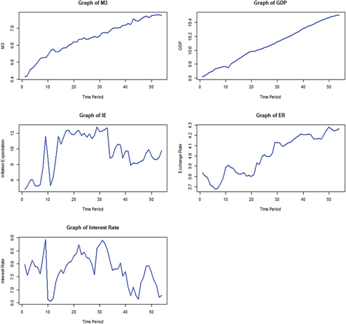
Table 3. Descriptive statistics

Variables	Min	Max	1.Qu.	3.Qu.	Mean	Median	Stdev	Skew	Kurt
LnM3	6.427	7.157	6.749	7.041	6.883	6.890	0.200	−0.448	−0.718
LnY	9.618	10.507	9.855	10.324	10.083	10.074	0.269	−0.026	−1.274
${\pi }^e$	4.800	12.800	8.250	11.700	9.565	9.700	2.369	−0.464	−0.922
LnER	3.675	4.278	3.829	4.173	4.009	4.018	0.188	−0.194	−1.475
r	6.539	8.927	7.402	8.184	7.767	7.833	0.632	−0.221	−0.718

Notes: Min stands for minimum, Max for maximum, 1.Qu. is the first quartile, 3.Qu. is the third quartile, Stdev is the standard deviation, Skew stands for skewness, and Kurt depicts kurtosis.

Source: Authors’ calculation

3.2. The ARDL or bounds testing approach to cointegration

The present study examines the existence of a short-run and long-run dynamic relationship between real money balance and its covariates and its stability based on the general specification in Equation (1)(1) $LnM{3}_t={\beta }_0+{\beta }_{1}Ln{Y}_t+{\beta }_2{r}_t+{\beta }_{3}LnE{R}_t+{\beta }_4{\pi }^e$(1) . To this end, the autoregressive distributed lag (ARDL) model, developed by Pesaran et al. (2001), is utilized. Pesaran et al. (2001) suggest a single equation cointegration concept known as ARDL or bounds testing approach to cointegration. It takes missing lag values into account, in turn, helps to avoid the spurious regression problem. The ARDL model has several advantages, for instance, its flexibility in use in context with the integration of the series, whether series are stationary at I(0) or I(1) or I(1)/I(0), in all cases this test is applicable, but series should not be of order I(2) or beyond otherwise the computed F-statistic by Pesaran et al. (2001) will not be valid (Pesaran et al., 2001). Furthermore, this model is appropriate even in the small sample size, confirmed by the Monte Carlo simulation technique (Pesaran & Shin, 1995). Finally, a dynamic unrestricted error correction model (UECM) can be derived from the ARDL bounds testing approach with the help of simple linear transformation. This is because the UECM is nothing but the reparameterization of the ARDL model. Therefore, the derivation of the UECM integrates the short-run dynamics with the long-run equilibrium relationship without losing any information about the long-run. The empirical structure of the long-run relationship in the bounds testing approach can be investigated with the help of the following UECM:

(2) $\begin{array}{rl}& \mathrm{\Delta }LnM{3}_t=c_{01}+\sum _{i=1}^{n1}{\varphi }_{1i}\mathrm{\Delta }LnM{3}_{t-i}+\sum _{i=0}^{n2}{\varphi }_{2i}\mathrm{\Delta }Ln{Y}_{t-i}+\sum _{i=0}^{n3}{\varphi }_{3i}\mathrm{\Delta }{r}_{t-i}+\sum _{i=0}^{n4}{\varphi }_{4i}\mathrm{\Delta }LnE{R}_{t-i}\\ & +\sum _{i=0}^{n5}{\varphi }_{5i}\mathrm{\Delta }{{\pi }^e}_{t-i}+{\beta }_{1}LnM{3}_{t-1}+{\beta }_{2}Ln{Y}_{t-1}+{\beta }_3{r}_{t-1}+{\beta }_{4}LnE{R}_{t-1}+{\beta }_5{{\pi }^e}_{t-1}+{\epsilon }_t\end{array}$(2)

Wherein Equation (2)(2) $\begin{array}{rl}& \mathrm{\Delta }LnM{3}_t=c_{01}+\sum _{i=1}^{n1}{\varphi }_{1i}\mathrm{\Delta }LnM{3}_{t-i}+\sum _{i=0}^{n2}{\varphi }_{2i}\mathrm{\Delta }Ln{Y}_{t-i}+\sum _{i=0}^{n3}{\varphi }_{3i}\mathrm{\Delta }{r}_{t-i}+\sum _{i=0}^{n4}{\varphi }_{4i}\mathrm{\Delta }LnE{R}_{t-i}\\ & +\sum _{i=0}^{n5}{\varphi }_{5i}\mathrm{\Delta }{{\pi }^e}_{t-i}+{\beta }_{1}LnM{3}_{t-1}+{\beta }_{2}Ln{Y}_{t-1}+{\beta }_3{r}_{t-1}+{\beta }_{4}LnE{R}_{t-1}+{\beta }_5{{\pi }^e}_{t-1}+{\epsilon }_t\end{array}$(2) , ∆ is the first difference operator, variables are as defined earlier, $c_{01}$is the intercept term, t subscript shows time, ${\varphi }_{1i}$- ${\varphi }_{5i}$are the coefficients of short-run dynamics, ${\beta }_1$ - ${\beta }_5$ represent the coefficients of the long-run relationship, and${\epsilon }_t$represents error terms which follow the white noise process.

The first step in ARDL, to confirm a long-run relationship among the variables under study, is to estimate Equation (2)(2) $\begin{array}{rl}& \mathrm{\Delta }LnM{3}_t=c_{01}+\sum _{i=1}^{n1}{\varphi }_{1i}\mathrm{\Delta }LnM{3}_{t-i}+\sum _{i=0}^{n2}{\varphi }_{2i}\mathrm{\Delta }Ln{Y}_{t-i}+\sum _{i=0}^{n3}{\varphi }_{3i}\mathrm{\Delta }{r}_{t-i}+\sum _{i=0}^{n4}{\varphi }_{4i}\mathrm{\Delta }LnE{R}_{t-i}\\ & +\sum _{i=0}^{n5}{\varphi }_{5i}\mathrm{\Delta }{{\pi }^e}_{t-i}+{\beta }_{1}LnM{3}_{t-1}+{\beta }_{2}Ln{Y}_{t-1}+{\beta }_3{r}_{t-1}+{\beta }_{4}LnE{R}_{t-1}+{\beta }_5{{\pi }^e}_{t-1}+{\epsilon }_t\end{array}$(2) using the ordinary least squares (OLS) method. The F-statistic is used to check the existence of the long-run relationship by utilizing the significance of the lagged level of variables. In Equation (2)(2) $\begin{array}{rl}& \mathrm{\Delta }LnM{3}_t=c_{01}+\sum _{i=1}^{n1}{\varphi }_{1i}\mathrm{\Delta }LnM{3}_{t-i}+\sum _{i=0}^{n2}{\varphi }_{2i}\mathrm{\Delta }Ln{Y}_{t-i}+\sum _{i=0}^{n3}{\varphi }_{3i}\mathrm{\Delta }{r}_{t-i}+\sum _{i=0}^{n4}{\varphi }_{4i}\mathrm{\Delta }LnE{R}_{t-i}\\ & +\sum _{i=0}^{n5}{\varphi }_{5i}\mathrm{\Delta }{{\pi }^e}_{t-i}+{\beta }_{1}LnM{3}_{t-1}+{\beta }_{2}Ln{Y}_{t-1}+{\beta }_3{r}_{t-1}+{\beta }_{4}LnE{R}_{t-1}+{\beta }_5{{\pi }^e}_{t-1}+{\epsilon }_t\end{array}$(2) , the null hypothesis of no cointegration is presented as H₀: ${\beta }_1={\beta }_2={\beta }_3={\beta }_4={\beta }_5=0$against alternative H₁:${\beta }_1\ne {\beta }_2\ne {\beta }_3\ne {\beta }_4\ne {\beta }_5\ne 0$. Pesaran et al. (2001) describe the lower and upper critical bound values as the two sets of critical values. The conclusion is made with F-statistic. If the F-statistic exceeds the upper critical bound value, in that case, the null hypothesis of no cointegration is rejected. If it falls below the lower critical bound, we fail to reject the null of no cointegration. Finally, if it lies between the lower and upper critical bounds, the results will be inconclusive. In this case, as Boutabba (2014) mentions, following Kremers et al. (1992) and Banerjee et al. (1998), the error correction term will help establish cointegration.

The second step, provided the long-run relationship exists, is to estimate the long-run model for LnM3 by utilizing Equation (3)(3) $LnM{3}_t=c_{01}+\sum _{i=1}^{n1}{\delta }_{1i}LnM{3}_{t-i}+\sum _{i=0}^{n2}{\delta }_{2i}Ln{Y}_{t-i}+\sum _{i=0}^{n3}{\delta }_{3i}{r}_{t-i}+\sum _{i=0}^{n4}{\delta }_{4i}LnE{R}_{t-i}+\sum _{i=0}^{n5}{\delta }_{5i}{\pi }^e+{\mu }_t$(3) . This Equation is estimated by using the appropriate lag length criterion.

(3) $LnM{3}_t=c_{01}+\sum _{i=1}^{n1}{\delta }_{1i}LnM{3}_{t-i}+\sum _{i=0}^{n2}{\delta }_{2i}Ln{Y}_{t-i}+\sum _{i=0}^{n3}{\delta }_{3i}{r}_{t-i}+\sum _{i=0}^{n4}{\delta }_{4i}LnE{R}_{t-i}+\sum _{i=0}^{n5}{\delta }_{5i}{\pi }^e+{\mu }_t$(3)

In the third step, the study extracts the short-run dynamic parameters by estimating an error correction model (ECM) associated with long-run estimates. The ECM model is stated as follows:

(4) $\begin{array}{rl}& \mathrm{\Delta }LnM{3}_t=c_{01}+\sum _{i=1}^{n1}{\varphi }_{1i}\mathrm{\Delta }LnM{3}_{t-i}+\sum _{i=0}^{n2}{\varphi }_{2i}\mathrm{\Delta }Ln{Y}_{t-i}+\sum _{i=0}^{n3}{\varphi }_{3i}\mathrm{\Delta }{r}_{t-i}+\sum _{i=0}^{n4}{\varphi }_{4i}\mathrm{\Delta }LnE{R}_{t-i}\\ & +\sum _{i=0}^{n5}{\varphi }_{5i}\mathrm{\Delta }{{\pi }^e}_{t-i}+\psi EC{T}_{t-1}+{\mu }_t\end{array}$(4)

In Equation (4)(4) $\begin{array}{rl}& \mathrm{\Delta }LnM{3}_t=c_{01}+\sum _{i=1}^{n1}{\varphi }_{1i}\mathrm{\Delta }LnM{3}_{t-i}+\sum _{i=0}^{n2}{\varphi }_{2i}\mathrm{\Delta }Ln{Y}_{t-i}+\sum _{i=0}^{n3}{\varphi }_{3i}\mathrm{\Delta }{r}_{t-i}+\sum _{i=0}^{n4}{\varphi }_{4i}\mathrm{\Delta }LnE{R}_{t-i}\\ & +\sum _{i=0}^{n5}{\varphi }_{5i}\mathrm{\Delta }{{\pi }^e}_{t-i}+\psi EC{T}_{t-1}+{\mu }_t\end{array}$(4) , ${\varphi }_{1i},{\varphi }_{2i},{\varphi }_{3i},{\varphi }_{4i},{\varphi }_{5i}$are the coefficients of short-run dynamics. ECT is the error correction term derived from the long-run relationship, and $\psi$ is the coefficient of ECT, which depicts the speed of adjustment. It measures the speed with which the response variable returns to a steady-state equilibrium path over time in the long-run due to the shocks in the explanatory variables.

3.3. Dynamic simulations of ARDL model

The ARDL model developed by Pesaran et al. (2001) offers an effective and consistent estimate. However, as the literature has developed, several other new capabilities are introduced over time in the recent econometric techniques to strengthen the robustness and consistency of an econometric model. Likewise, Philips (2018) addresses, in the dynamically simulated ARDL, the difficulties that arise owing to the complex dynamic structure of the ARDL model. The ARDL model may have a fairly complex lag structure because of the appearances of other entities into the model specification, for instance, with lags, contemporaneous values, first differences, and lagged first differences of the independent (and sometimes the dependent) variable (Jordan & Philips, 2018, p. 14). Although, in an ARDL (1, 1) model set up the short-run and long-run effects may be easier to interpret. However, as the model specification becomes more complex, understanding the short-, medium-, and long-run effects becomes difficult.

To overcome the complexities of the ARDL model and better interpret the substantive significance of the results, Philips (2018) introduces the dynamically simulated ARDL approach of cointegration. It simplifies numerous complex structures while testing the model coefficients’ significance through meaningful counterfactual scenarios. This kind of approach to ARDL modelling estimates, simulates, and generates an impulse response function, which helps us visualize the effect of a counterfactual change in a regressor at a time, holding all else equal, using stochastic simulation techniques (Jordan & Philips, 2018). The dynamic simulation approaches are more popular in revealing the substantive time series model’s results wherever the coefficients often have non-intuitive or “hidden” interpretations (Jordon and Philips, 2018 quote Breunig & Busemeyer, 2012).

The dynamic simulations of ARDL first run a regression using OLS. It takes 1000 draws (or simulations can be extended depending upon users) of the vector of parameters from a multivariate normal distribution. Based on the work of Jordan and Philips (2018), the following dynamic simulation of the unrestricted error correction mechanism is utilized in the present study.

(5) $\begin{array}{rl}& \mathrm{\Delta }LnM{3}_t=c_{01}+{\delta }_{0}LnM{3}_{t-i}+{\theta }_1\mathrm{\Delta }Ln{Y}_t+{\delta }_{1}Ln{Y}_{t-1}+{\theta }_2\mathrm{\Delta }{r}_t+{\delta }_2{r}_{t-1}+{\theta }_3\mathrm{\Delta }LnE{R}_t+{\delta }_{3}LnE{R}_{t-1}\\ & \\ & +{\theta }_4\mathrm{\Delta }{{\pi }^e}_t+{\delta }_4{{\pi }^e}_{t-1}+{\mu }_t\end{array}$(5)

In Equation (5)(5) $\begin{array}{rl}& \mathrm{\Delta }LnM{3}_t=c_{01}+{\delta }_{0}LnM{3}_{t-i}+{\theta }_1\mathrm{\Delta }Ln{Y}_t+{\delta }_{1}Ln{Y}_{t-1}+{\theta }_2\mathrm{\Delta }{r}_t+{\delta }_2{r}_{t-1}+{\theta }_3\mathrm{\Delta }LnE{R}_t+{\delta }_{3}LnE{R}_{t-1}\\ & \\ & +{\theta }_4\mathrm{\Delta }{{\pi }^e}_t+{\delta }_4{{\pi }^e}_{t-1}+{\mu }_t\end{array}$(5) , ${\delta }_0$ denotes the error correction term (ECT) ${\theta }_1$ to ${\theta }_4$capture the short-run coefficients and ${\delta }_1$ to ${\delta }_4$depict a long-run coefficient for each of the regressors, respectively. To implement the dynamic ARDL error correction term algorithm for the given specification in Equation (5)(5) $\begin{array}{rl}& \mathrm{\Delta }LnM{3}_t=c_{01}+{\delta }_{0}LnM{3}_{t-i}+{\theta }_1\mathrm{\Delta }Ln{Y}_t+{\delta }_{1}Ln{Y}_{t-1}+{\theta }_2\mathrm{\Delta }{r}_t+{\delta }_2{r}_{t-1}+{\theta }_3\mathrm{\Delta }LnE{R}_t+{\delta }_{3}LnE{R}_{t-1}\\ & \\ & +{\theta }_4\mathrm{\Delta }{{\pi }^e}_t+{\delta }_4{{\pi }^e}_{t-1}+{\mu }_t\end{array}$(5) , the present study conducts 5000 simulations for the vector of variables from the multivariate normal distribution.

4. Empirical analysis

As a first step in the empirical analysis, the series’s integration is checked using the unit root test. The unit root testing is being carried out to ensure that none of the variables follows the I(2) process. Table 4 presents the Augmented Dickey–Fuller (ADF) test by Dickey and Fuller (1981) and Phillips–Perron (PP) test by Phillips and Perron (1988). The results show that all variables are non-stationary at the level form except r, which is level stationary. However, the non-stationary series becomes stationary after the first difference. Thus, the present study has witnessed a mixture of the I(0) and I(1) processes. Moreover, this kind of integration of the series provides a strong justification for employing the ARDL model.

Table 4. Unit root test results

Variables	ADF Statistics				PP Statistics
	Level	p-Value	First Diff	p-Value	Level	p-Value	First Diff	p-Value
LnM3	3.591	0.99	−2.484	0.01	4.665	1.00	−5.651	0.00
LnY	−2.153	0.50	−6.689	0.00	−2.555	0.30	−6.697	0.00
${\pi }^e$	−2.467	0.34	−7.705	0.00	−2.022	0.58	−7.610	0.00
LnER	−2.723	0.23	−5.418	0.00	−3.040	0.13	−5.420	0.00
r	−2.614	0.09	-	-	−2.690	0.08	-	-

Notes: First diff and p-Value stand for first difference and probability value, respectively

Source: Authors’ calculation

In the next step, the cointegration between the response variable and its covariates is checked. The computed F-statistic and critical values from Pesaran et al. (2001) are presented in Panel A of Table 5. The result shows that the computed F-statistic value is greater than the upper critical bound value at a 10% significance level. Therefore, we reject the null hypothesis of no cointegration among the variables, which implies a long-run cointegrating relationship among real money balance, inflation expectation, exchange rate, scale, and opportunity cost variables. This result is akin to the findings of Adil et al. (2020b) in the case of India, wherein they establish a cointegrating relationship between real narrow and broad money measures and their covariates using the bounds testing approach to cointegration in the post-economic reform period. Conversely, we contradict Moosa’s (1992) finding. The study mentions unstable M2 money measure in the case of India before the economic reform period.

Table 5. Results of bounds test for cointegration, diagnostic testing, and parameter stability test

Panel A: Bounds testing result
Test Statistics	Value		K
F-statistic	3.95		4
Critical bounds values
	10%		5%			1%
Bounds	I(0)	I(1)	I(0)		I(1)	I(0) 4.244	I(1)
F-statistic	2.578	3.710		3.068	4.334		5.726
Panel B: Series of diagnostic testing
Diagnostic test	Jarque-Bera	Breusch-Pagan/Cook-Weisberg				Breush-Godfrey		Ramsey RESET
Statistic	2.154		0.980			14.454		1.780
p-value	0.34		0.32			0.00		0.17
Panel C: Parameters Stability Test
Method	Test Statistic		Critical Values
			10%			5%		1%
Recursive	0.370		0.850			0.948		1.143
OLS	0.360		1.224			1.358		1.628

Notes: RESET stands for regression specification error test.

Source: Authors’ calculation

In the next step, as suggested by Jordan and Philips (2018, p.15), before applying the dynamically simulated ARDL, a priori, it is mandatory to determine the order of integration of the variables through unit-root testing, a series of diagnostic testing on the model, and use of information criteria to identify the best fitting lagged-difference structure, which is used to purge autocorrelation and to ensure the residuals are white noise. Hence, in Panel B, the series of tests are applied where the estimated ARDL model passes almost every diagnostic test. Finally, we investigate the structural stability of the long-run parameters of the model using the cumulative sum (CUSUM) of recursive residuals test developed by Brown et al. (1975). We reject the null hypothesis of stable parameters provided the test statistic is greater than the critical value (alternatively, if the parameter stability is being checked through the graph—which is done in Figures 2 and 3, the plotted recursive residuals, depicted with a red line, go outside the critical bandwidth, depicted with grey areas).

Figure 2. Plot of recursive CUSUM.

Source: Authors’ calculation

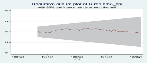
Figure 3. Plot of OLS CUSUM.

Source: Authors’ calculation

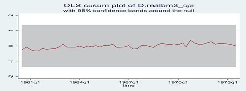
Furthermore, the study has also conducted the ordinary least squares (OLS) residuals-based CUSUM test. In Panel C, the recursive and OLS residuals-based CUSUM test statistics are lower than the 1% critical values. In the case of graphical representation, depicted in Figures 2 and 3, both test statistics are within the confidence interval and do not breach the confidence limits, which implies no structural instability in the long-run parameter of the model under the study period. All in all, all the diagnostic and stability tests depict that the ARDL model specification presents a reliable and stable estimate which can be utilized for the policy analysis.

The next step is to find the impact of an independent actor of the model on the response variable. To this end, the dynamically simulated ARDL model is estimated; the results are presented in Table 6. In Panel A, the short-run coefficients are presented. The ECT is statistically significant at a 1% significance level with a negative coefficient sign. The lagged value of ECT in the short-run model appears with a coefficient of −0.234, which directly implies the monotonic convergence to the equilibrium path. The coefficient of the ECT shows that the response variable will come back towards its steady-state path equilibrium with the speed of 23.4% per quarter due to the disturbances created by its covariates or any other external positive or negative shock. Furthermore, the significant ECT reinforces the long-run relationship among variables in the model. Focusing on just a significant variable—the inflation forecast variable, which is a main concern in the present study, is significant at a 5% significance level. A one-unit change in the inflation forecast induces a 0.5% change in the real money balance. It implies that economic agents consider future inflation as an opportunity cost of holding real money balance and maintain their portfolios by focusing on future inflation. The current result supports the rational expectation theory very well. Therefore, agents update their information set and behave rationally to avoid the inflation tax or shoe leather cost of inflation. The significant inflation parameter of the present study favours the finding of Murad et al. (2021) study. The study reveals a significant short-run inflation rate in India using the ARDL approach of cointegration.

Table 6. Dynamically simulated ARDL results

Variables	Coefficients	SE	t-statistic	p-value
Panel A: Short-run coefficients
ΔLnYt	0.092	0.248	0.370	0.71
Δ rt	0.004	0.006	0.560	0.58
Δ${\pi }^e$t	−0.005	0.003	−2.060	0.05
ΔLnERt	0.037	0.069	0.530	0.60
ECTt-1	−0.234	0.088	−2.650	0.01
Panel B: Long-run coefficients
LnM3t-1	−0.811	0.158	−5.130	0.00
LnYt-1	0.202	0.087	2.330	0.03
rt-1	0.005	0.006	0.730	0.47
${\pi }^e$t-1	−0.008	0.003	−3.130	0.00
LnERt-1	0.027	0.070	0.390	0.70
Adj. R-squared	0.533	Simulations	5000
F-statistic p-value	0.00	Observations	50

Note: All abbreviations are defined in Table 2

Source: Authors’ calculation

The long-run coefficient estimates are presented in panel B. All the variables are statistically significant at their conventional significance level except interest rate and exchange rate. Focusing on significant structural parameters, the inflation forecast is negatively significant at a 1% significance level and greater in magnitude. Thus, in the long-run, also, the inflation forecast is consistent with the short-run coefficient estimates. The long-run significant inflation parameter supports the finding of Murad et al. (2021) in India, where they find consistently significant inflation parameter in the short- and long-run both during the entire sample period. Furthermore, we find the significant structural parameter of the scale variable in the long-run, which supports the result of Adil et al. (2020b) in India. They empirically examine real narrow and broad monetary measures using the ARDL bounds testing approach to cointegration and find a significant long-run scale variable.

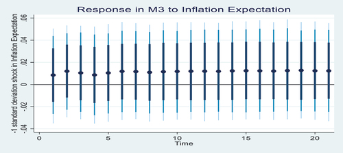
Philips (2018) designs the dynamic simulations of the ARDL model, which is envisaged to be superior compared to the simple ARDL model by Pesaran et al. (2001). It simplifies the complexities in the ARDL and helps us understand and interpret the estimates through plots. The plots of dynamically simulated estimates visualize the short-run and long-run impacts of a shock in explanatory variables on the response variable. The impulse is created by giving a positive/negative standard deviation shock to the explanatory variables. In the present study, to generate the estimates, 5000 simulations for the vector of variables from a multivariate normal distribution are being executed. The graphical illustrations of the dynamic ARDL simulations have been shown in Figures 4, 5, 6, and 7. The plots are observed over 30-time horizons along with ± one standard deviation shock activated on an explanatory variable at a time in the money demand specification to initiate a counterfactual change in the independent variable.

Figure 4. The impulse response plot for GDP.

Note: This figure shows one standard deviation positive shock in GDP and its impact on M3. The dots show the mean change in the predicted value from the sample mean. The shaded area shows (from darkest blue to lightest blue) the 75%, 90%, and 95% confidence intervals.

Source: Authors’ calculation

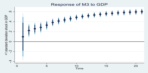
Figure 5. The impulse response plot for GDP.

Note: This figure shows one standard deviation negative shock in GDP and its impact on M3. The dots show the mean change in predicted value from the sample mean. The shaded area shows (from darkest blue to lightest blue) the 75%, 90%, and 95% confidence intervals.

Source: Authors’ calculation

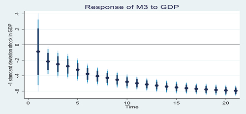
Figure 6. The impulse response plot for inflation expectation.

Note: This figure shows one standard deviation positive shock in inflation expectation and its impact on M3. The dots show the mean change in the predicted value from the sample mean. The shaded area shows (from darkest blue to lightest blue) the 75%, 90%, and 95% confidence intervals.

Source: Authors’ calculation

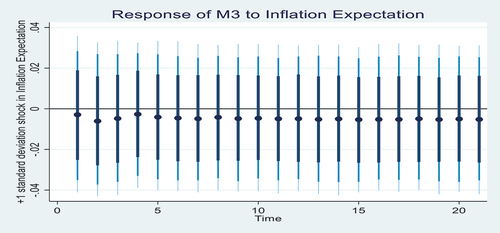
Figure 7. The impulse response plot for inflation expectation.

Note: This figure shows one standard deviation negative shock in inflation expectation and its impact on M3. The dots show the mean change in predicted value from the sample mean. The shaded area shows (from darkest blue to lightest blue) the 75%, 90%, and 95% confidence intervals.

Source: Authors’ calculation

In Figure 4, the effect on M3 to one standard deviation positive shock in GDP has shown across 30-time horizons. The change is slightly higher in the short run but eventually becomes smaller in the long-run. The positive shock in GDP leads to an increase in the real money balance by 0.1 compared to the pre-shock equilibrium level in the short-run before stabilizing at around 0.6, in the long-run, above the pre-shock equilibrium level. However, in the later horizon of time, the impact of GDP produces a smaller impact that is not statistically significant in the long-run. Conversely, in Figure 5, the negative shock to GDP depicts its impact on M3. The negative shock reduces the amount of money holding by 0.1, in the short-run, compared to the pre-shock equilibrium level before stabilizing at around 0.6 below the pre-shock equilibrium level. Again, one standard deviation negative shock at 30-time horizons produces a higher increase that is statistically significant in the short-run, which eventually increases to a change in the predicted value of 0.6 over the long-run, a statistically insignificant increase.

In Figure 6, the effect on M3 to one standard deviation positive shock in inflation forecast has shown across 30-time horizons. The change is constant throughout the period. The positive shock in the inflation forecast reduces M3 by 0.01 compared to the pre-shock equilibrium level in the short-run. It remains consistent in magnitude at around 0.01, below the pre-shock equilibrium level in the long-run. Conversely, in Figure 7, the negative shock to inflation expectation depicts its impact on M3. The negative shock increases the amount of money holding by 0.01, in the short-run, compared to the pre-shock equilibrium level, and it remains consistent at around 0.01 above the pre-shock equilibrium level. After giving an impulse to each explanatory variable, the response of all the variables orthogonally depicts the results as per economic theory, which carries an important policy implication.

5. Summary and concluding remarks

As a part of highlighting the significance of money in the formulation of rule-based monetary policy such as flexible inflation targeting, the present study aims to examine the short- and long-run money demand relationship and its stability in India for the period 2006: Q3 to 2019: Q4. To this end, the study has deployed the dynamically simulated ARDL approach of cointegration. The results show well-specified MDF in India after incorporating the inflation forecast variable as one of the essential determinants among other covariates. The bounds testing approach of cointegration confirms a long-run relationship among variables, while the recursive and OLS residuals-based CUSUM tests confirm the stability of the money demand equation. Furthermore, the dynamically simulated impulse response also supports the economic relationship quite well among variables.

Against the above backdrop, our findings carry a significant policy implication. Under the monetary policy committee of India, which has been discussed in the minutes of the last several meeting, the current FIT framework adopts an accommodative stance of policy. Wherein the price stability, eventually economic stability, is still a top priority along with output growth. The RBI considers inflation forecast as an intermediate target variable to achieve the macroeconomic goal of price stability. Since in the present study, the MDF is stable and well specified by the inflation forecast variable. Therefore, based on the current findings, the study recommends that the RBI should accord monetary aggregate as an important indicator or information variable to focus its ultimate macroeconomic goal variable, that is, inflation targeting. Consequently, the present study supports the argument that while conducting monetary policy, the money should be envisaged as an essential instrument, especially in a low inflation scenario when the policy rate might be ineffective, for instance, zero lower bound problem.

The above policy implication is aligned with the monetary policy strategy of the European Central Bank (ECB). Wherein the soundness of monetary policy still focuses on the importance of money growth. Notably, the ECB continues to assign a prominent role to money in its monetary policy strategy. In what the ECB calls its “two-pillars strategy”, as mentioned in its report (ECB, 2004, p. 55). One pillar is considered as ‘economic analysis, which focuses on short-to-medium-term determinants of the development of price level. The second pillar is ‘monetary analysis, which focuses on a medium-to-long-term outlook for inflation, and this pillar examines the long-run causal link between money and price level. Thus, in the second pillar, money has been accorded prominent importance to target the macroeconomic goal variable, for instance, price stability.

Declaration of Conflicting Interests

The author declared no potential conflicts of interest concerning the research, authorship and/or publication of this article.

Disclosure statement

No potential conflict of interest was reported by the authors.

Additional information

Funding

The authors received no direct funding for this research.

Notes on contributors

Masudul Hasan Adil

Masudul Hasan Adil is currently affiliated with the School of Management, Indian Institute of Technology (IIT) Mandi, Himachal Pradesh, India. He has worked as Post-doctoral Fellow in the Department of Economics, IIT Bombay and HSS in the IIT Palakkad. He has completed his PhD in Monetary Economics from the Mumbai School of Economics & Public Policy, Mumbai, India, and MPhil in the area of Public Finance from the School of Economics, University of Hyderabad, Hyderabad, India. His research interests focus in the area of Monetary Economics, Macroeconomics, and Time Series Analysis.

Neeraj R. Hatekar

Neeraj Hatekar is a Professor in the School of Development, Azim Premji University Bengaluru, India. His areas of interest and expertise are Long Term Economic Change, Large Scale Data Sets, and Understanding Interface between Geography and Economic Policy.

Notes

1. For a detailed discussion of money through new Keynesian and new monetarist perspectives, see Adil et al. (2021).

2. For a detailed discussion of different monetary policy regimes in India, see Adil and Rajadhyaksha (2021).

3. For a detailed discussion, see RBI (2014). Although the RBI has paved the way for inflation targeting for a long back which is evident with the series of incidences, for instance, the talk about inflation targeting in India started in the late 1990s and got momentum after the Reserve Bank of New Zealand’s Dr. Donald T Brash speech on the L. K. Jha memorial lecture series on June 1999 in Mumbai; the report on Banking Sector Reforms and Rajan (2007) report on Financial Sector Reforms have also recommended for implementing the inflation targeting; as an RBI Governor, Dr. Rajan has set up an expert committee that is a landmark report on inflation targeting headed by Patel (2014) which has recommended and finalized the framework for inflation targeting; finally, after a considerable amount of discussion, formally the flexible inflation targeting framework is adopted in India with the signing of the Monetary Policy Framework Agreement between the Government of India and the RBI on February 2015.

4. The theory posits that economic agents decide based on human rationality, information available to them, and their past experiences. Nowadays, economists use the rational expectations theory to explain anticipated economic factors, such as inflation and interest rates.

References

- Adil, M. H., Haider, S., & Hatekar, N. R. (2020a). Empirical Assessment of Money Demand Stability Under India’s Open Economy: Non-linear ARDL Approach. Journal of Quantitative Economics, 18(4), 891–20. https://doi.org/10.1007/s40953-020-00203-1
- Adil, M. H., Haider, S., & Hatekar, N. R. (2020b). Revisiting Money Demand Stability in India: Some Post-reform Evidence (1996–2016). The Indian Economic Journal, 66(3–4), 326–346. https://doi.org/10.1177/0019466220938930
- Adil, M. H., Hatekar, N., Fatima, S., Nurudeen, I., & Mohammad, S. (2022). Money Demand Function. Journal of Economic Integration, 37(1), 93–120. https://doi.org/10.11130/jei.2022.37.1.93
- Adil, M. H., Hatekar, N. R., & Ghosh, T. (2021). The Role of Money in the Monetary Policy: A New Keynesian and New Monetarist Perspective. In W. A. Barnett & B. S. Sergi (Eds.), Environmental, Social, and Governance Perspectives on Economic Development in Asia (pp. 37–67). Emerald Publishing Limited.
- Adil, M. H., Hatekar, N., & Sahoo, P. (2020c). The Impact of Financial Innovation on the Money Demand Function: An Empirical Verification in India. Margin: The Journal of Applied Economic Research, 14(1), 28–61. https://doi.org/10.1177/0973801019886479
- Adil, M. H., & Rajadhyaksha, N. (2021). Evolution of monetary policy approaches: A case study of Indian economy. Journal of Public Affairs, 21(1), e2113. https://doi.org/10.1002/pa.2113
- Arango, S., & Nadiri, M. I. (1981). Demand for money in open economies. Journal of Monetary Economics, 7(1), 69–83. https://doi.org/10.1016/0304-3932(81)90052-0
- Arrau, P., & De Gregorio, J. (1993). Financial innovation and money demand: Application to Chile and Mexico. The Review of Economics and Statistics, 75(3), 524–530. https://doi.org/10.2307/2109469
- Bahmani-Oskooee, M., Bahmani, S., Kones, A., & Kutan, A. M. (2015). Policy uncertainty and the demand for money in the United Kingdom. Applied Economics, 47(11), 1151–1157. https://doi.org/10.1080/00036846.2014.993138
- Bahmani-Oskooee, M., & Ng, R. C. W. (2002). Long-run demand for money in Hong Kong: An application of the ARDL model. International Journal of Business and Economics, 1(2), 147.
- Ball, L. (2001). Another look at long-run money demand. Journal of Monetary Economics, 47(1), 31–44. https://doi.org/10.1016/S0304-3932(00)00043-X
- Ball, L. (2012). Short-run money demand. Journal of Monetary Economics, 59(7), 622–633. https://doi.org/10.1016/j.jmoneco.2012.09.004
- Banerjee, A., Dolado, J., & Mestre, R. (1998). Error‐correction mechanism tests for cointegration in a single‐equation framework. Journal of Time Series Analysis, 19(3), 267–283. https://doi.org/10.1111/1467-9892.00091
- Barnett, W. A., Ghosh, T., & Adil, M. H. (2022). Is money demand really unstable? Evidence from Divisia monetary aggregates. Economic Analysis & Policy, 74, 606–622. https://doi.org/10.1016/j.eap.2022.03.019
- Belongia, M. T., & Ireland, P. N. (2019). The demand for Divisia Money: Theory and evidence. Journal of Macroeconomics, 61, 103128. https://doi.org/10.1016/j.jmacro.2019.103128
- Boutabba, M. A. (2014). The impact of financial development, income, energy and trade on carbon emissions: Evidence from the Indian economy. Economic Modelling, 40, 33–41. https://doi.org/10.1016/j.econmod.2014.03.005
- Breunig, C., & Busemeyer, M. R. (2012). Fiscal austerity and the trade-off between public investment and social spending. Journal of European Public Policy, 19(6), 921–938. https://doi.org/10.1080/13501763.2011.614158
- Brown, R. L., Durbin, J., & Evans, J. M. (1975). Techniques for testing the constancy of regression relationships over time. Journal of the Royal Statistical Society, Series B, 37(2), 149–192. https://doi.org/10.1111/j.2517-6161.1975.tb01532.x
- Deev, O., & Hodula, M. (2016). The long-run superneutrality of money revised: The extended European evidence.
- Dekle, R., & Pradhan, M. (1999). Financial liberalization and money demand in the ASEAN countries. International Journal of Finance & Economics, 4(3), 205–215. https://doi.org/10.1002/(SICI)1099-1158(199907)4:3<205:AID-IJFE107>3.0.CO;2-G
- De La Fuente, G. G., De La Horra, L. P., & Perote, J. (2020). The demand for Divisia money in the United States: Evidence from the CFS Divisia M3 aggregate. Applied Economics Letters, 27(1), 41–45. https://doi.org/10.1080/13504851.2019.1606403
- Dickey, D. A., & Fuller, W. A. (1981). Likelihood ratio statistics for autoregressive time series with a unit root. Econometrica: Journal of the Econometric Society, 49(4), 1057–1072. https://doi.org/10.2307/1912517
- ECB. (2004). The Monetary Policy of the ECB. European Central Bank.
- Friedman, M. (1970). A theoretical framework for monetary analysis. Journal of Political Economy, 78(2), 193–238. https://doi.org/10.1086/259623
- Funke, N., & Thornton, J. (1999). The demand for money in Italy, 1861–1988. Applied Economics Letters, 6(5), 299–301. https://doi.org/10.1080/135048599353276
- Goldfeld, S. M., Duesenberry, J., & Poole, W. (1973). The demand for money revisited. Brookings Papers on Economic Activity, 1973(3), 577–646. https://doi.org/10.2307/2534203
- Goldfeld, S. M., Fand, D. I., & Brainard, W. C. (1976). The case of the missing money. Brookings Papers on Economic Activity, 1976(3), 683–739. https://doi.org/10.2307/2534372
- Hossain, A. A. (2019). How justified is abandoning money in the conduct of monetary policy in Australia on the grounds of instability in the money‐demand function? Economic Notes: Review of Banking, Finance and Monetary Economics, 48(2), e12131. https://doi.org/10.1111/ecno.12131
- James, G. A. (2005). Money demand and financial liberalization in Indonesia. Journal of Asian Economics, 16(5), 817–829. https://doi.org/10.1016/j.asieco.2005.08.003
- Jonson, P. D. (1976). Money and economic activity in the open economy: The United Kingdom, 1880-1970. Journal of Political Economy, 84(5), 979–1012. https://doi.org/10.1086/260493
- Jordan, S., & Philips, A. Q. (2018). Cointegration testing and dynamic simulations of autoregressive distributed lag models. The Stata Journal, 18(4), 902–923. https://doi.org/10.1177/1536867X1801800409
- Judd, J. P., & Scadding, J. L. (1982). The search for a stable money demand function: A survey of the post-1973 literature. Journal of Economic Literature, 20(3), 993–1023.
- King, M. (2001). No money, no inflation the role of money in the economy. Économie internationale, 4(4), 111–131. https://doi.org/10.3917/ecoi.088.0111
- Kremers, J. J., Erksson, N. R., & Dolado, J. J. (1992). The power of cointegration tests. Oxford Bulletin of Economics and Statistics, 54(3), 325–347. https://doi.org/10.1111/j.1468-0084.1992.tb00005.x
- Laidler, D. E. (1982). Monetarist perspectives. Harvard University Press.
- Laidler, D. E. (1993). The demand of money: Theories, evidence and the problems. Harper Collins.
- Mohanty, D. (2011). Changing contours of monetary policy in India. Speech by Shri Deepak Mohanty, Executive Director, Reserve Bank of India, delivered at the Royal Monetary Authority of Bhutan, Thimpu on.
- Moosa, I. A. (1992). The demand for money in India: A cointegration approach. The Indian Economic Journal, 40(1), 101. https://doi.org/10.1177/0019466219920106
- Murad, S. W., Salim, R., & Kibria, M. G. (2021). Asymmetric effects of economic policy uncertainty on the demand for money in India. Journal of Quantitative Economics, 19, 451–470.
- Muralikrishna Bharadwaj, B., & Pandit, V. (2010). Policy reforms and stability of the money demand function in India. Margin: The Journal of Applied Economic Research, 4(1), 25–47. https://doi.org/10.1177/097380100900400102
- Nelson, E. (2008). Why money growth determines inflation in the long-run: Answering the Woodford critique. Journal of Money, Credit, and Banking, 40(8), 1791–1814. https://doi.org/10.1111/j.1538-4616.2008.00183.x
- Payne, J. E. (2003). Post stabilization estimates of money demand in Croatia: Error correction model using the bounds testing approach. Applied Economics, 35(16), 1723–1727. https://doi.org/10.1080/0003684032000152871
- Pesaran, M. H., & Shin, Y. (1995). An autoregressive distributed lag modelling approach to cointegration analysis (Vol. 9514). Department of Applied Economics, University of Cambridge.
- Pesaran, M. H., Shin, Y., & Smith, R. J. (2001). Bounds testing approaches to the analysis of level relationships. Journal of Applied Econometrics, 16(3), 289–326. https://doi.org/10.1002/jae.616
- Philips, A. Q. (2018). Have your cake and eat it too? Cointegration and dynamic inference from autoregressive distributed lag models. American Journal of Political Science, 62(1), 230–244. https://doi.org/10.1111/ajps.12318
- Phillips, P. C., & Perron, P. (1988). Testing for a unit root in time series regression. Biometrika, 75(2), 335–346. https://doi.org/10.1093/biomet/75.2.335
- Ramachandran, M. (2004). Do broad money, output, and prices stand for a stable relationship in India? Journal of Policy Modeling, 26(8–9), 983–1001. https://doi.org/10.1016/j.jpolmod.2004.08.008
- RBI. (2014). Report of the Expert Committee to Revise and Strengthen the Monetary Policy Framework. Reserve Bank of India, Retrieved from: https://www.rbi.org.in/SCRIPTs/PublicationReportDetails.aspx?UrlPage=&ID=743
- Romer, D. H. (2000). Keynesian macroeconomics without the LM curve. Journal of Economic Perspectives, 14(2), 149–169. https://doi.org/10.1257/jep.14.2.149
- Taylor, J. B. (2009). The financial crisis and the policy responses: An empirical analysis of what went wrong. National Bureau of Economic Research. No. w14631
- Thornton, D. L. (2014). Monetary policy: Why money matters (and interest rates don’t). Journal of Macroeconomics, 40, 202–213. https://doi.org/10.1016/j.jmacro.2013.12.005
- Woodford, M. (2000). Monetary policy in a world without money. International Finance, 3(2), 229–260. https://doi.org/10.1111/1468-2362.00050