Time-varying connectedness and contagion between commodity prices and exchange rate in Sub-Saharan Africa

Abstract

Market participants, policymakers, and practitioners might have ignored the connection between global commodities and the currency markets in sub-Saharan Africa and the potential for contagion at various time scales. We examine the degree of time-varying connectivity and contagion between commodities and the exchange rates of sub-Saharan African countries (SSA). We use the Barunik and Krehlik (BK18) spillover index on monthly data from 1990 to 2019 to illustrate the dynamic connectivity in the time and frequency domains. The BK18 captures the nonlinear, nonstationary, asymmetric, and time-dependent comovements in the relationship. Our analysis indicates that the relationship between commodity returns and exchange rates in Sub-Saharan Africa (SSA) is both time- and frequency-dependent, but stronger at higher frequencies. We observe that, among the three commodities, only crude oil is a dominant spillover propagator. The exchange rates of South Africa dominate spillover transmission among metal-producing countries, and those of Cote d’Ivoire dominate agricultural-producing countries. The dynamic results reveal significant spillovers between commodities and exchange rates during economic turmoil, indicating contagion among the markets. Since uncertainty spillover is more severe amid market upheaval, investors should use their awareness of market dynamics and fluctuations to protect their holdings from lower asset returns. Policymakers should keep a close eye on spillovers because they endanger cross-market connections.

Keywords:

• commodity prices
• exchange rate
• time-varying connectedness
• contagion
• spillovers

1. Introduction

The financial economics literature has shown significant interest in connectedness and contagion, mainly driven by financial catastrophes like the Asian, Mexican, and Russian crises, the 2007/2008 global financial crisis (GFC), the 2013 oil price drop, and the COVID-19 pandemic (see, for instance, Boako & Alagidede, 2017; Diebold & Yilmaz, 2009; Jiang et al., 2022). The growing interdependence of countries as economic partners or neighbours has also opened the door to shock spillovers and, as a result, interest in contagion (Owusu Junior et al., 2020). Again, high market integration, especially for nations in the same economic bloc, contributes to high interest in contagion research and financial market expansion as investors seek secure assets (Tiwari et al., 2019).

The numerous academic interests in contagion have generated a debate on what constitutes financial contagion. From the perspective of fundamental contagion theorists, contagion occurs when there is shock transmission from one country or market to another through the real sector or macroeconomic factors (Bekaert et al., 2005; Forbes & Rigobon, 2002; Pritsker, 2000). On the contrary, the pure contagion theorists are of the belief that when shocks are transmitted from one country or market to another without any idiosyncratic factors, there is contagion (see Dornbusch et al., 2000; Kaminsky et al., 2003). The lack of clarity in the meaning of contagion led Forbes and Rigobon (2002) to propose “shift contagion” (SC), which is a significant shift in cross-market linkages. To them, a cross-market linkage without any significant change in spillover constitutes connectedness. Despite the contribution of SC, the definition and measurement of contagion are still the subject of an ongoing and contentious debate. Contagion is therefore an empirical issue that is contextual in nature; hence, this study seeks to examine the connectedness and contagion between global commodity prices (CP) and exchange rates (ER) in SSA. In line with Forbes and Rigobon (2002), we separate connectedness from contagion and make inferences about any possible decoupling between the two markets.

The focus on commodities and ER is motivated by the high dependence of countries in SSA on commodity exports for revenue. Indeed, nine out of 10 countries in SSA are classified as commodity dependent (United Nations Conference on Trade and Development, 2021), and since these commodities are traded mainly in US dollars on the international market, there is a high probability of shocks emanating from commodity prices to ER in SSA. At the same time, these countries see commodities as assets that can be relied on to hedge their currencies, especially in turbulent times. As a result, understanding the dynamics of interdependence and possible contagion between these two variables will be helpful in the hedging and risk management decisions of policymakers in SSA.

Moreover, information from crises like the GFC and the recent COVID-19 pandemic usually triggers a reaction from market participants and agents to look for alternative assets to put in their portfolios, either for hedging purposes or for diversification. These economic agents could either be rational or irrational, and because of the heterogeneity in their behaviour, they may be following the heterogeneous market hypothesis (HMH) by Muller et al. (1993) or the adaptive market hypothesis proposed by Lo (2004). The idea behind these theories is that the differences among investors cause them to operate at different investment horizons as they respond to volatility differently. Investors’ behaviour is thus frequency-varying over time, contrary to the proposition of the efficient market hypothesis (EMH), which sees investors behave similarly. Market participants seeking an efficient portfolio, particularly during times of crisis, look for assets that are uncorrelated or negatively correlated to provide a safe haven (Baur & Lucey, 2010). This is because contagion between assets diminishes portfolio diversification possibilities since it increases correlation (Gulko, 2002).

Financial markets in Africa, including the forex and stock markets, have become attractive to global investors because there is a perception fuelled by some studies that the African markets, like many in other developing economies, are decoupled from global economic activities (see Kose & Prasad, 2010; Kose et al., 2008; World Economic Outlook, 2007). These studies posit that economic activities in advanced markets and the developing and emerging worlds are uncorrelated, contrary to the views of contagion theorists. The implication is that returns from FX markets in SSA and the global commodities market will not be related normally; that is, they will not be correlated. This belief has led to increased capital inflows to SSA markets (Atenga & Mougoué, 2021; oro Owen, 2017; World Bank Group, 2018). The question then is: do the currency markets in SSA offer any diversification opportunities to commodity investors, and do commodities provide hedging potential for currencies in SSA? The answer to the question hinges on the nature of any possible connectedness or contagion between the two variables, and since not much is known in this direction, this study seeks to provide a possible guide to investors and policymakers.

Further, several studies on financial contagion in the financial economics literature have focused on contagion between stock markets (Caporin et al., 2018; Diebold & Yilmaz, 2009; Owusu Junior et al., 2020), between commodities (Bouri et al., 2017; Ji & Fan, 2012; Shen et al., 2022), between currencies (see Antonakakis, 2012; Bubák et al., 2011; Huynh et al., 2020; Kočenda & Moravcová, 2019; Salisu et al., 2018), and between commodities and stocks (Agyei & Bossman, 2023; Alagidede et al., 2021). Yet, contagion between commodity markets and currency markets has received limited attention. The few exceptions, like Dai et al. (2020) and Jiang et al. (2022), focused on only major currencies at the expense of those of weaker economies. The situation in SSA is even worse, as studies on contagion between global commodities and exchange rates (ER) hardly exist. Mention can be made of Katusiime (2018), but apart from the study being limited to only one country (Uganda), no differentiation was made between connectedness and contagion. This gap needs immediate attention due to the high dependence of countries in SSA on commodity exports.

Additionally, previous connectedness and contagion studies between commodities and ER in SSA have concentrated on linear and static time analysis in line with EMH with little or no attention to the time-frequency dimension. This is a significant gap because Muller et al. (1993) found that agents in financial markets respond to volatility differently at different investment horizons, corresponding to high, medium, and low frequencies. Understanding the frequency dynamics of connectedness is critical to finding the origins of connectivity in an economic system since economic shocks have various impacts on variables at different frequencies and intensities. Again, measuring connections in the frequency domain provides another source for managing systemic risk between assets (Baruník & Křehlík, 2018). Moreover, most prior studies have relied on GARCH, transfer entropy, and DY12 methods. Although these methods contain information about static time-domain analysis, they are limited in their ability to examine the frequency information of contagion over time. There is therefore a need to utilise a more robust method capable of capturing the dynamic behaviour of market agents.

This study differs from others by focusing on returns as the source of contagion in commodity-dependent developing countries and making the following contributions: First, the study provides novel understandings of the ways in which dependence and contagion spread both within and between ERs in SSA and between global commodities and ERs in SSA by disaggregating return volatility. Such analysis provides more information about the heterogeneous behaviour of investors, which varies across different times (short-, medium-, and long-terms) and may be hidden from studies focusing on composite behaviour (Owusu Junior & Gherghina, 2022). The information provided by the study is helpful to investors and policymakers for risk management.

Second, it examines the dynamic interdependence between commodities and ER at different frequencies (high, medium, and low) and over time. This provides information about how complex connections between CP and ER have evolved over time. Such analyses appeal to HMH, which has indicated that the differences in investor expectations and appetite for risk, among others, make them operate at different investment horizons at different times. Therefore, while institutional investors and monetary policy authorities are more interested in medium and low frequencies, which correspond to medium- and long-terms, speculators focus on high frequencies, which correspond to short-terms. Findings here will therefore be more useful to different participants in the markets making hedging decisions than other studies that focus on only time at the expense of time variation.

Third, we quantify connectedness and contagion using the non-parametric method of Baruník’s and Křehlík (2018) time-domain, frequency-domain, and time-frequency domain framework (BK18). This method captures non-linear and non-stationary returns. Non-stationarity and non-linearity are becoming important in spillover research. To the best of our knowledge, this method has not been applied to commodities and currency markets in SSA, as prior studies have mostly applied the Diebold and Yilmaz (2012) spillover index and GARCH methods, which are limited in accounting for the frequency dimension of the relationship. Again, BK18 accounts for causality in the frequency domain by using “within” connectivity, contrary to DY12. The BK18 considers composite and pairwise (bi-directional) spillover at different frequencies and timings. It estimates net spillovers by comparing “from” and “to” spillovers. BK18 calculates spillovers like several current studies (see Adam, 2013; Diebold & Yilmaz, 2009; Saiti et al., 2015). BK18’s contagion measurement is consistent with Forbes and Rigobon’s (2002) “shift contagion” measurement. It captures contagion asymmetry, which benefits investors and policymakers.

Fourth, we present evidence of currency market contagion in 27 commodity-producing and largely commodity-dependent SSA countries. Commodity-dependent countries need to know whether they should spend more time dealing with external shocks from global commodity prices or dealing with shocks from the exchange rates of other commodity-exporting countries within the continent. The use of three major commodities (oil, gold, and cocoa) and several countries provides a broader understanding of the situation in specific countries to aid investor and policy decision-making. The methods employed in this study (BK18) can determine the system’s most dominant contributor to spillovers. This is important for systemic risk management and portfolio diversification. By using BK18, the study can determine whether a specific country at a specific frequency is a net receiver of return shocks in pairs or as a whole, which other methods are unable to do.

Our findings show a significant time-varying frequency relationship between global commodities and currencies in SSA, with varied spillover contagion during crisis times. We observed that crude oil and cocoa are net transmitters of spillovers to exchange rates, but gold is a net recipient of spillovers. This finding creates room for gold to provide a hedge for the exchange rates of metal-exporting countries. According to market conditions, there are huge opportunities for diversification between commodities and SSA currency markets, as well as between pairs of SSA currencies in systems.

The paper continues as follows: Section 2 is a review of related works, and Section 3 looks at the material and methods. In the fourth section, we concentrate on the discussion of results from the estimation, while the fifth and final section concludes the study with recommendations.

2. Literature review

Despite the ongoing debate on the concept of contagion, empirical studies abound in the literature, with inconsistencies probably due to the multiplicity of measurements. Several studies in this area have concentrated on the return and volatility spillovers between the exchange rates of major currencies in the world, with varying outcomes. Bubák et al. (2011) conducted a study on volatility transmission between the currencies of Central European (CE) countries and the EUR/USD exchange rate, relying on model-free estimates of daily exchange rate volatility. The findings showed that in the Central European markets, there are statistically significant intra-day spillovers among the currencies. Except for the Czech Republic and Poland, there were no spillovers from EUR/USD markets to CE markets. In a study to examine the volatility spillover and exchange rate co-movement before and after the Euro introduction, Antonakakis (2012) utilised a VAR-based spillover index for major currencies in Europe and the US dollar. The results show that spillovers were important, but on average they were smaller after the euro was introduced than they were before. This shows that spillovers change over time and need to be looked at from time to time.

Similarly, Salisu et al. (2018) examined the return and volatility spillovers in the global exchange rate markets, focusing on the six most traded currency pairs (Aussie, Cable, Euro, Gropher, Loonie, and Swissy) in the world using daily data from January 1999 to December 2014. The result from the DY12 model indicates that interdependence exists among major currency pairs, but while return spillovers exhibit mild trends, volatility spillovers exhibit no trend at all. It must be pointed out that, apart from the study focusing on only the major currencies in the world, the analysis was only done in the time domain, which falls short of bringing out the total dynamics at different levels.

In a related study, Kočenda and Moravcová (2019) investigated spillovers, co-movement, and hedging costs in the EU forex markets with monthly data from 1999 to 2018. They concluded that correlation and spillovers were unstable; the correlation becomes negative during turbulent times, and cross-currency spillovers rise at times of crisis. Not only do their findings contradict some aspects of Antonakakis (2012), but they also assume a time-domain analysis. More recently, Huynh et al. (2020) considered the role of trade policy uncertainties in studying connectedness and spillovers in the foreign exchange market over the period from 1999 to 2019 for nine major US dollar exchange rate currencies. It came out that connectedness and spillovers are present only after considering trade policy, albeit at a higher level of volatility than the return. This study, just like previous studies, ignores the weaker currencies and is also limited to time-domain analysis.

Other contagion studies have focused on exchange rates and stock market relationships. For example, Lin (2012) focused on the emerging Asian market by studying the co-movement between exchange rates and stock markets. The autoregressive distributed lag (ARDL) was used, and the findings show that spillovers become stronger during crisis times, which is a sign of contagion during turbulent times. But while the study attempts to differentiate between connectedness and contagion, the method used is more linear in nature, which defeats the nonlinear nature of financial data like stock prices and exchange rates. In a similar vein, Moore and Wang (2014) examined the dynamic linkages between real exchange rates and stock returns, focusing on the US market and emerging Asian markets. Using the dynamic conditional correlation (DCC) approach, they discovered that trade balance is a key influencer of the relationship between Asian and US markets, while interest rate differential is the primary influencer on US markets. But, like Lin (2012), this study is limited by the fact that linear models cannot show the whole picture of what is going on.

Boako and Alagidede (2017) carried out a more thorough investigation into the existence of “shift contagion” in African stock markets using weekly data to examine extreme events (downside movement from the global exchange rate and developed stock markets). The conditional value at risk (CoVAR) based on the copula method was employed, and the findings show that, based on “shift contagion,” there is evidence of contagion from some developed stock markets and exchange rates to African stock markets. They argued that shocks do not happen only during crisis times but can also happen post-crisis, so there is “delayed-shift contagion.” While we share the view that there can be a delay in contagion, a simple extension of the study period does not necessarily defeat the implicit assumptions of the SC since the SC still captures shocks after the crisis period. However, the mathematical assumptions in implementing shift contagion (SC) might be its main weakness, an issue this thesis seeks to correct.

Some studies have used multi-scale analysis to study the nonlinear connection between commodities and foreign exchange markets, albeit with a focus on major currency markets and mostly one commodity (oil or gold). For instance, Benhmad (2012) studied the nonlinear causality between oil prices and the US dollar, relying on the wavelet approach. The findings show that the causality relationship was bi-directional and varied over frequency but was unidirectional at the first frequency, running only from oil to exchange rate. In a similar fashion, Reboredo and Rivera-Castro (2014) examined the importance of gold to exchange rate risk management in terms of hedging and downside risk. The analysis was done at different investment horizons using wavelet multiresolution analysis. The findings show that over the period 2000–2013, the depreciation of gold and the US dollar had a positive dependence on other currencies used in the study at all-time scales. Despite these two studies using the same approach but with different commodities, the findings are not consistent for both. While the former does not obtain a consistent relationship at all frequencies, the latter does. This creates room for an assessment of the relationship between different commodities and different currencies. Moreover, the wavelet method used in both studies has the probability of smearing the energy of the decomposed frequencies, thus making their reliability suspect.

Uncertainty in the results is also evidenced in Wen et al. (2017), who sought to assess the nonlinear Granger causality and time-varying effect between crude oil and the US dollar. In this study, multiple methods were applied, including the Hiemstra and Jones test, the Diks and Panchenko test, and the time-varying parameter structural autoregressive model (TVPSAR). The finding of the study was that the exchange rate does not cause the oil price, but rather the other way around: the exchange rate has a more stable negative effect on the oil price. Despite the multiple methods used in Wen et al. (2017), none of them has the capability of proper decomposition to present frequency-level information.

In a recent study, Yıldırım et al. (2022) investigated the volatility transmission between real exchange rates and real commodity prices for three emerging economies: Mexico, Indonesia, and Turkey. The study suggests that a bidirectional causality exists between the CP and ER but that the relationship varies with time and that volatility transfer disappears in times of crisis, particularly during the COVID-19 pandemic. Yıldırım et al. (2022) also revealed that, though both precious metals and oil have safe-haven potential for the exchange rate, risk transfer from oil only happens in Indonesia and not in the other two countries. One weakness of this study is that it is a time-domain study with no frequency dimension. Again, the study also confirms the importance of studying different commodities and different exchange rates due to the inconsistencies in the outcomes for both oil and gold in the same study.

Other studies on co-movement and connectedness have concentrated on other sectors and assets. One such study is that of Athari and Hung (2022), who focused on the asset class co-movement pre- and post-COVID-19 eras with specific emphasis on equity, digital assets, commodities, and fixed income. Using daily data from 2017 to 2021, the results from the wavelet analysis indicate that co-movement among assets during the COVID-19 pandemic intensified relative to the pre-COVID period. The problem is that the study relied on commodity indexes instead of specific commodities, making it difficult for specific country policies. Kirikkaleli and Athari (2020) studied bank credit supply and economic growth in Turkey using data from 1993 to 2017. Findings from the wavelet analysis concluded that ownership structure plays a significant role in the connection between credit supply and economic growth in the short and long run. A related study by Athari et al. (2021) focused on credit ratings for economic risk in Balkan countries. Using data from 1999 to 2019, the results show that while there is one-way causality between credit rating and the economies of Bulgaria and Croatia in the long run, feedback causality exists between credit rating and the economies of Greece, Slovenia, and Romania. While these studies show the importance of studying connections between assets on different time scales, they did not focus on the currency market with an emphasis on some European countries. There is therefore a need to provide evidence from the African currency market and global commodities due to their important contribution to global commodity exports.

Contagion studies on African currency markets have primarily been linear or time-domain analyses. For instance, Katusiime (2018) investigated price volatility spillovers from commodities to the exchange rate in Uganda using dynamic conditional correlation (DCC), constant conditional correlation (CCC), and time-varying conditional correlation (TVCC). The study found that market interconnectedness and volatility spillover are generally low but increase during times of crisis, using data from January 1992 to April 2017. Atenga and Mougoué (2021) study the return and volatility spillover to African currencies using data from 2000 to 2019. The empirical results of the DY12 model show that African currencies respond more to themselves than to global factors, except for Botswana, Morocco, Tunisia, and South Africa, which may be linked to other currencies.

The forgoing literature presents the following issues and weaknesses: (1) that most empirical evidence has focused on major currencies in developed economies; (2) that there are inconsistencies in empirical findings when different commodities are used for different currency markets or even when the same commodity is used for different currencies; (3) that many existing studies concentrate on linear interaction; (4) that there is a paucity of empirical evidence on time-variation, particularly in SSA; and (5) that there is a lack of studies testing the “decoupling hypothesis” in the frequency domain of the currency market in SSA from global CP. Based on the weaknesses identified in the literature, this study fills the gaps by: (1) using three commodities (oil, gold, and cocoa) and the exchange rates of 27 commodity-producing countries in SSA; (2) appealing to the HMH and presenting evidence in the frequency domain; and (3) employing the BK18 approach. In the process, we differentiate between connectedness and contagion, similar to Forbes and Rigobon (2002) and Owusu Junior et al. (2020), and make an inference about the decoupling hypothesis in SSA. We take frequency heterogeneity into account in our analysis, which gives investment and policy decisions a more complete picture.

3. Material and methods

3.1. Methodology

We provide details of the Baruník and Křehlík (2018) spillover methods, which was relied on to achieve the purpose of the study. Baruník and Křehlík (2018) spillover method, commonly called BK18 was motivated by Diebold and Yilmaz’s (2012) method (DY12), which estimates connectedness among variables in the time domain. Barunik and Krehlik extended the DY model to incorporate the frequency domain in estimating connectedness. The benefit of the BK18 method is its ability to account for connections in the time domain, frequency domain, and time-frequency domain. The DY12 calculates connectedness from generalised forecast error variance decompositions (GFEVDs), which are based on the matrix of vector autocorrelation (VAR) model of local covariance stationarity. For instance, if we denote $K-variance$ process as $Y_t=(y_{1,t,}\dots ,y_{k,t}{)}^{\prime }$ at $t=1,\dots ,T$, then, the $VA{R}_{\left(\rho \right)}$ may be expressed as;

(1) $Y_t=\sum _{i=1}^p{\mathrm{\varnothing }}_i{y}_{t-1}+{ϵ}_t$(1)

From Equation (1)(1) $Y_t=\sum _{i=1}^p{\mathrm{\varnothing }}_i{y}_{t-1}+{ϵ}_t$(1) , ${\mathrm{\varnothing }}_i$ and ${ϵ}_t$ represent coefficient matrix and white noise respectively with (possibly non-diagonal) covariance matrix$\mathrm{\Pi }$. In the equation above, the system makes it possible to regress each of the variables on its own $\rho$ lags and the $\rho$ lags of other variables. This makes $\mathrm{\varnothing }$ have complete information of the connection between all the variables. It must be indicated that it is helpful to work with $\left(KxK\right)$ matrix $(I_K-{\mathrm{\varnothing }}_{1}L-\dots -{\mathrm{\varnothing }}_p{L}^p)$ with identity $I_K$. The $\left(L\right)$ and the$(L^p)$ represent the lag and lag polynomial respectively. In this process, if the root of $\left|\theta \left(Z\right)\right|$ lies outside the unit circle, then the VAR process contains a vector moving average $\left(i.e.,\mathrm{M}\mathrm{A}\left(\mathrm{\infty }\right)\right)$ expressed as

(2) $Y_t=\psi \left(L\right){ϵ}_{t,}$(2)

Where $\psi \left(L\right)$ is an infinitely lag polynomial. Building on Diebold and Yilmaz (2012) the GFEVD can be expressed as;

(3) $({\mathrm{\Theta }}_H{)}_{j,k}=\frac{{\sigma }_{kk}^{-1}{\mathrm{\Sigma }}_{h=0}^H{({\psi }_h\mathrm{\Pi })}_{j.k}{)}^2}{{\mathrm{\Sigma }}_{h=0}^H{({\psi }_h{\mathrm{\Pi }}_{h{ }^{\mathrm{\prime }}})}_{j.k}}$(3)

Where ${\psi }_h$ is $KxK$ matrix having a coefficient corresponding to $h$ lags$\left(i.e.,h=1,\dots ,H\right)$ and ${\sigma }_{kk}={\left(\mathrm{\Pi }\right)}_{k,k}$ and represent the contribution of the $k_{th}$ variable to the variance of the forecast error of the element $j$. It is worth noting that the sum of each row does not necessarily add up to one, so each element of the decomposition matrix is normalized as follows;

(4) $({\tilde{\mathrm{\Theta }}}_H{)}_{j.k}=\frac{{({\mathrm{\Theta }}_H)}_{j.k}}{{\mathrm{\Sigma }}_{k=1}^H{({\mathrm{\Theta }}_h)}_{j.k}}$(4)

It should be noted that $({\tilde{\mathrm{\Theta }}}_H{)}_{j.k}$ provides a pairwise connectedness measure from $j$ to $i$ at horizon $H$ that can be aggregated by design. The connectedness measure is defined by Diebold and Yilmaz (2012) as the amount of variance in forecasts contributed by errors other than own errors or the ratio of the sum of the off-diagonal element to the sum of the entire matrix, which is expressed as

(5) ${\mathrm{C}}_H=100\ast \frac{{\mathrm{\Sigma }}_{j\ne k}{({\tilde{\mathrm{\Theta }}}_H)}_{j.k}}{\mathrm{\Sigma }{\tilde{\mathrm{\Theta }}}_H}=100\ast \left(1-\frac{Tr\left\{{\tilde{\mathrm{\Theta }}}_H\right\}}{\mathrm{\Sigma }{\tilde{\mathrm{\Theta }}}_H}\right)$(5)

From (5), $Tr\left\{\ast \right\}$ is the trace operator, and the denominator stand for the sum of all the elements of ${\tilde{\mathrm{\Theta }}}_H$ Matrix. Accordingly, connectedness is the relative contribution of the other variables in the system to the forecast variances. Until now, the link between commodity prices and exchange rates has been clearly demonstrated in time domain. We can also measure spillovers from one country to another. Barunik and Krehlik extended the DY model to incorporate the frequency domain in estimating connectedness. As a foundation, if we consider a frequency response function $\psi (e{)}^{-i\omega }={\mathrm{\Sigma }}_h{e}^{-i\omega h}{\psi }_h$ of Fourier transformable coefficient ${\psi }_h$ with $i=\sqrt{-1}$, then, a spectral density of $Y_t$ at a frequency $\omega$ can be expressed as $MA\left(\mathrm{\infty }\right)$ filters series as follows;

(6) $S_{y\left(\omega \right)}=\sum _{h=\mathrm{\infty }}^{\mathrm{\infty }}E\left(Y{ }^{\mathrm{\prime }}{Y}_{t-h}\right)e^{-i\omega h}=\psi \left(e^{-i\omega }\right)\mathrm{\Pi }\psi { }^{\mathrm{\prime }}\left(e^{+i\omega }\right)$(6)

The power spectrum $S_{y\left(\omega \right)}$ expresses how the variance of the $Y_t$ is distributed over the frequency component $\omega$ and is very important in understanding the frequency dynamics. The generalized causation spectrum over $\omega ϵ=\left(-\pi ,\pi \right)$ is expressed as:

(7) ${\left(\mathcal{F}\left(\omega \right)\right)}_{j,k}=\frac{{\sigma }_{kk}^{-1}|\psi \left(e^{-i\omega }\right){\mathrm{\Pi }}_{j,k}{|}^2}{\psi \left(e^{-i\omega }\right)\mathrm{\Pi }\psi { }^{\mathrm{\prime }}\left(e^{+i\omega }\right){)}_{j,j}}$(7)

The ${\left(\mathcal{F}\left(\omega \right)\right)}_{j,k}$ indicate the portion of the $ith$ variable at a given frequency $\omega$ due to shocks in the $kth$ variable. From that, we can interpret the quantity as within-frequency causation based on the denominator which shows a spectrum of$jth$ variable at a frequency of $\omega$. The most logical thing to do now is to weigh ${\left(\mathcal{F}\left(\omega \right)\right)}_{j,k}$ by the frequency share of the variance of the $jth$ variable to get the natural decomposition of GFEVD to frequencies. This is expressed as

(8) ${\mathrm{\Gamma }}_j=\frac{\psi \left(e^{-i\omega }\right)\mathrm{\Pi }\psi { }^{\mathrm{\prime }}\left(e^{+i\omega }\right){)}_{j,j}}{\frac{1}{2\pi }{\int }_{-\pi }^{\pi }{(\psi \left(e^{-i\lambda }\right)\mathrm{\Pi }\psi { }^{\mathrm{\prime }}\left(e^{+i\lambda }\right))}_{j,j}d\lambda }$(8)

The weighted function defined in (8) is the power of $\left(jth\right)$ variable at a given frequency which sums up the value of real numbers through to $2\pi$. Indeed, it is appropriate to measure connectedness over time horizons if we have proper financial application. Therefore, measuring connectedness at different frequency bands instead of just at a single frequency is very necessary. So as a general representation, if we have a frequency band $d=\left(a,b\right):a,bϵ\left(-\pi ,\pi \right),a<b,$ then, the GFEVDs can be expressed as

(9) $({\mathrm{\Theta }}_d{)}_{j,k}=\frac{1}{2\pi }\underset{a}{\overset{b}{\int }}{\mathrm{\Gamma }}_j\left(\omega \right){(\mathcal{F}\left(\omega \right))}_{j,k}d\omega$(9)

From (9), a scale generalized variance decomposition can be expressed over the same frequency band $d$ as follows.

(10) $({\tilde{\mathrm{\Theta }}}_d{)}_{j,k}=({\mathrm{\Theta }}_d{)}_{j,k}/{\sum }_k({\mathrm{\Theta }}_{\mathrm{\infty }}{)}_{j,k}$(10)

Consequently, (9) and (10) respectively define the within-frequency and frequency connectedness over $d$ as follows

(11) $C_d^w=100.\left(1-\frac{{\mathrm{T}}_r\left\{{\tilde{\mathrm{\Theta }}}_d\right\}}{\mathrm{\Sigma }{\tilde{\mathrm{\Theta }}}_d}\right)$(11)

(12) $C_d^F=100.\left(\frac{\mathrm{\Sigma }{\tilde{\mathrm{\Theta }}}_d}{\mathrm{\Sigma }{\tilde{\mathrm{\Theta }}}_{\mathrm{\infty }}}-\frac{{\mathrm{T}}_r\left\{{\tilde{\mathrm{\Theta }}}_d\right\}}{\mathrm{\Sigma }{\tilde{\mathrm{\Theta }}}_{\mathrm{\infty }}}\right)=C_d^w.\left(\frac{\mathrm{\Sigma }{\tilde{\mathrm{\Theta }}}_d}{\mathrm{\Sigma }{\tilde{\mathrm{\Theta }}}_{\mathrm{\infty }}}\right)$(12)

Based on the estimation of Baruník and Křehlík (2018), $C_d^w$ measures the connectedness within a frequency band which is exclusively weighted by the power of the series. The $C_d^F$ on the contrary decomposes the original connectedness into separate parts which add up to the original connectedness measure. In this study, the frequency bands $\left(\pi +0.00001,\pi /4,\pi /12,0\right)$ as seen in Baruník and Křehlík (2018) and Tiwari et al. (2019) are used.

3.2. Data

The data used as input for the VAR analysis were the monthly return series for three commodities and the exchange rate. The series covered log returns from January 1990 to December 2019 for commodity-exporting countries in sub-Saharan Africa following IMF classification. Three commodities (gold, cocoa, and crude oil) were utilised for the study based on their massive revenue contribution to countries in SSA, and data on commodity prices were gleaned from the World Bank commodity price database, commonly called the “Pink Sheet”. These three commodities were selected from three categories: metal commodities, agricultural commodities, and energy commodities, respectively.

Data on exchange rates were sourced from the International Financial Statistics (IFS) database of the IMF for countries included in the study. The exchange rate is a measure of the rate between a particular country’s currency and the US dollar. Countries selected for the study were grouped into three groups based on their level of dependence on a particular commodity or commodities. The connection between gold and ER was calculated for metal-exporting countries; that of cocoa and ER for agricultural-exporting countries was done; and finally, the estimation of oil and exchange rates for energy-exporting countries was done.

Table 2 presents the stationarity test results and the series’ descriptive statistics. Also, results on the graphical behaviour of both the original and return series of the commodities are presented in Figure A1 in Appendix A. The graphs in Figure A1 show that the original series’ behaviour is unstable. For instance, commodity prices recorded sharp price drops between 2007 and 2008. The sharp change in price may have been a result of the GFC over the period. The return series of commodities has stable trends with some volatility in the study space. The augmented Dickey-Fuller (ADF) test by Dickey and Fuller (1979) and the Phillips-Perron (PP) test by Phillips and Perron (1988) indicated that all the return series were stationary at the 1% significant level. In conducting the analysis, the entire set of 359 data points was used to calculate the spillover in the time domain and the frequency domain. The data were then rolled over to account for the time-frequency domain, with a window size of 100 and a forecast horizon of 12 months. The lag selected for the VAR model was done in order to minimise the AIC. It is worth noting that, when using the BK18 method, it is unnecessary to exogenously designate the start and end times of the crisis when using the rolling window approach. By visualising the resulting spillover indices, we can take into consideration significant alterations in the shape of spillovers as we roll the data across the whole sample period (Yilmaz, 2010). The Diebold-Yilmaz and Barunik-Krehlik spillover frameworks have this as a major advantage over other methods.

Table 1 displays the selected bands’ interpretations in the BK18 framework. The selected bands were to help in accounting for time-frequency spillovers in the short-, medium-, and long-terms, respectively.

Table 1. Time-scale and frequency interpretation

BK18
Band	Frequency	Months	Interpretation
d1	3.14 ~ 0.79	1 ~ 4	Short-term
d2	0.79 ~ 0.26	4 ~ 12	Medium-term
d3	0.26 ~ 0.00	12 ~ ∞	Long-term

Table 2. Summary statistics and test of stationarity

	Obs	mean	SD	skewness	kurtosis	N.test	ADF	PP
Commodity price returns
Oil return	359	0.0032	0.0851	−0.3516	2.494	0.960***	−11.264***	−13.548***
Gold return	359	0.0036	0.0349	0.3655	1.548	0.979***	−14.446***	−17.068***
Cocoa return	359	0.0025	0.0581	0.0861	0.810	0.993*	−12.588***	−16.315***
Oil Producing countries
Angola	359	0.03	0.1074	8.072	83.352	0.318***	−9.283***	−13.437***
Cameroon	359	0.002	0.044	11.382	179.649	0.440***	−12.868***	−17.561***
Ghana	359	0.0145	0.0343	2.877	18.905	0.603***	−11.288***	−18.037***
Mauritania	359	0.0042	0.0271	5.833	74.915	0.481***	−14.081***	−20.293***
Nigeria	359	0.0102	0.0813	13.757	216.648	0.164***	−13.301***	−17.993***
Metal producing countries
Botswana	359	0.0049	0.027	0.629	8.921	0.879***	−12.622***	−15.922***
Burundi	359	0.0066	0.0226	2.412	13.326	0.770***	−12.979***	−16.32***
DRC	359	0.0335	0.1165	5.100	36.868	0.460***	−11.446***	−14.799***
Ghana	359	0.0145	0.0343	2.8769	18.905	0.603***	−11.288***	−18.037***
Guinea	359	0.0075	0.0301	−0.291	21.679	0.619***	−10.946***	−13.068***
Mali	359	0.002	0.044	11.382	179.649	0.440***	−12.868***	−17.562***
Mauritania	359	0.0042	0.0271	5.833	74.915	0.481***	−14.081***	−20.293***
Mozambique	359	0.012	0.0325	1.204	4.708	0.866***	−9.438***	−12.416***
Namibia	359	0.0048	0.0371	0.803	3.570	0.946***	−11.993***	−16.833***
Rwanda	359	0.0069	0.04	10.792	128.665	0.230***	−12.832***	−17.631***
South Africa	359	0.0048	0.0343	0.627	5.062	0.939***	−12.221***	−14.119***
Tanzania	359	0.0069	0.0201	2.768	17.693	0.739***	−12.231***	−13.512***
Zambia	359	0.0183	0.0645	2.0261	9.809	0.782***	−11.406***	−15.819***
Agricultural producing countries
Comoros	359	0.0012	0.0321	6.044	76.385	0.687***	−12.502***	−16.228***
Cote d’Ivoire	359	0.002	0.044	11.382	179.650	0.440***	−12.868***	−17.561***
Eswatini	359	0.0048	0.0343	0.627	5.062	0.939***	−12.221***	−14.119***
Ethiopia	359	0.0076	0.0484	16.558	293.408	0.108***	−13.446***	−18.756***
Gambia	359	0.0052	0.029	−0.718	8.463	0.817***	−12.309***	−15.92***
Ghana	359	0.0145	0.0343	2.877	18.905	0.603***	−11.288***	−18.038***
Kenya	359	0.0043	0.03	1.346	17.525	0.717***	−10.869***	−12.352***
Madagascar	359	0.0069	0.0413	6.451	80.716	0.635***	−11.614***	−15.78***
Malawi	359	0.0157	0.0482	3.920	22.979	0.610***	−11.46***	−11.882***
Mauritius	359	0.0025	0.0183	0.702	3.775	0.937***	−11.817***	−12.483***
Nigeria	359	0.0102	0.0813	13.757	216.649	0.164***	−13.301***	17.993***
Seychelles	359	0.0026	0.0391	11.407	184.424	0.353***	−11.695***	−14.945***
Uganda	359	0.0064	0.025	0.734	3.743	0.921***	−9.637***	−13.493***

Note: The asterisk (***), (**), and (*) represent the level of significance at 1%, 5%, and 10% respectively. N. test stands for normality test and the ADF and PP tests include both intercept and trend.

4. Empirical results

In this section, emphasis is placed on discussing the results obtained from the Baruník and Křehlík (2018) framework. The analysis is presented in two sections. The first part focuses on the results from the frequency domain, classified as static analysis (Baruník & Křehlík, 2018; Diebold & Yilmaz, 2012). The analysis then proceeds to the second section for the results of the rolling window, which is described as the time-frequency variation by the extant literature (see Baruník & Křehlík, 2018; Diebold & Yilmaz, 2014; J. M. Polanco-Martínez, 2019; J. Polanco-Martínez et al., 2018).

4.1. Static frequency connectedness

In this static analysis, three frequencies are selected, and the results are presented in three Tables 3, 4 and 5, for oil and energy-exporting countries, gold and metal-exporting countries, and cocoa and agricultural-exporting countries, respectively. The expected contribution from commodity/exchange rate j innovations to the forecast error variance in commodity/exchange rate i is represented by the ijth entry. The proportion of the forecast error variance attributable to the commodity’s or exchange rate’s own innovations is represented by diagonal entries (i = j) (shocks). These are the table’s greatest values, which makes sense given their size.

Table 3. Total spillover and net spillover indices between oil and exchange rate of energy-producing countries in SSA

	Oil Return	Angola	Cameroon	Ghana	Mauritania	Nigeria	FROM_ABS^a	FROM_WTH^b
Band 1: 3.14 to 0.79 corresponds to 1 month to 4 months
Oil Return (OR)	56.68	0.23	0.68	0.18	0.59	1.75	0.57	0.84
Angola (AN)	0.48	49.12	0.05	0.38	0.15	0.19	0.21	0.31
Cameroon (CM)	0.56	0.04	67.66	3.71	0.48	0.12	0.82	1.21
Ghana (GH)	0.52	0.08	1.64	65.87	0.03	0.31	0.43	0.63
Mauritania (MT)	1.32	0.15	0.04	5.01	72.63	0.28	1.13	1.67
Nigeria (NR)	1.03	0.27	0.17	0.11	0.34	73.88	0.32	0.47
TO_ABS	0.65	0.13	0.43	1.57	0.27	0.44	3.48
TO_WTH	0.96	0.19	0.63	2.31	0.39	0.65		5.14
Net	0.08	−0.08	−0.39	1.14	−0.87	0.12
Band 2: 0.79 to 0.26 correspond to 4 months to 12 months
Oil Return	23.94	0.29	0.48	0.1	0.28	0.61	0.29	1.47
Angola	0.2	26.36	0.03	0.25	0.07	0.02	0.09	0.47
Cameroon	1.22	0.01	15.17	1.18	0.25	0.06	0.45	2.26
Ghana	0.32	0.18	0.76	18.11	0.00	0.04	0.22	1.08
Mauritania	1.11	0.03	0.06	1.17	11.01	0.06	0.41	2.03
Nigeria	0.33	0.04	0.07	0.09	0.09	15.94	0.11	0.53
TO_ABS^a	0.53	0.09	0.23	0.47	0.11	0.13	1.57
TO_WTH^b	2.65	0.46	1.17	2.33	0.57	0.65		7.84
Net	0.24	−0.00	−0.22	0.25	−0.29	0.024
Band 3: 0.26 to 0.00, correspond to 12 months to infinity
Oil Return	13.13	0.21	0.23	0.04	0.18	0.40	0.18	1.44
Angola	0.2	22.11	0.03	0.28	0.06	0.02	0.10	0.81
Cameroon	0.83	0.00	7.86	0.70	0.15	0.00	0.28	2.30
Ghana	0.18	0.21	0.49	1.27	0.00	0.00	0.15	1.19
Mauritania	0.72	0.04	0.05	0.72	5.59	0.01	0.26	2.09
Nigeria	0.13	0.00	0.04	0.06	0.06	7.34	0.05	0.39
TO_ABS^a	0.34	0.08	0.14	0.30	0.08	0.07	1.01
TO_WTH^b	2.82	0.62	1.14	2.45	0.62	0.59		8.23
Net	0.17	−0.02	−0.14	0.15	−0.18	0.02

Note: ^aAbsolute to measure return spillovers from commodity/country j to other countries. Absolute from measure return spillovers from other countries to commodity/country j. ^bWithin to measure return spillovers from commodity/country j to other countries, including from own innovation to commodity/country k. Within from measure return spillovers from other countries to commodity/country j, including from own innovation to commodity/country k (Tiwari et al., 2019). The three largest contributors to spillovers are in bold for all frequencies.

Table 4. Total spillover and net spillover indices between gold and exchange rate of metal-producing countries in SSA

	GR	BT	BU	DRC	GH	GU	ML	MT	MZ	NB	RW	SA	TZ	ZM	FROM_ABS^a	FROM_WTH^b
Band 1: 3.14 to 0.79 corresponds to 1 month to 4 months
Gold Return (GR)	57.8	3.34	0.34	0.23	1.03	0.18	0.77	0.59	0.24	2.56	0.20	3.12	0.60	0.51	0.98	1.51
Botswana (BT)	1.01	25.42	0.14	0.13	0.10	0.67	1.23	1.04	1.82	15.41	0.42	17.45	1.06	0.36	2.92	4.49
Burundi (BU)	0.77	0.37	59.75	0.92	0.67	1.38	1.41	1.64	0.25	0.30	0.31	0.35	0.24	0.49	0.65	1.00
DRC	0.41	0.25	2.11	55.18	0.11	0.40	0.08	0.24	0.14	0.09	0.57	0.13	0.30	0.37	0.37	0.57
Ghana (GH)	0.77	0.70	0.41	0.17	58.38	0.07	1.57	0.08	0.58	0.23	0.22	0.23	3.93	1.18	0.72	1.11
Guinea (GU)	0.79	1.96	0.10	0.09	0.26	51.77	0.10	1.92	0.13	1.07	0.02	1.40	0.33	0.18	0.60	0.92
Mali (ML)	1.03	2.54	0.56	0.28	2.90	0.14	53.88	0.41	0.35	1.70	0.62	1.91	2.49	2.81	1.27	1.95
Mauritania (MT)	0.90	2.94	0.87	0.31	4.22	0.91	0.13	59.03	1.06	2.19	0.23	2.77	0.83	0.43	1.27	1.96
Mozambique (MZ)	0.14	0.89	0.26	0.04	0.48	0.14	0.03	0.04	38.29	0.12	1.05	0.11	0.93	0.28	0.32	0.50
Namibia (NB)	0.81	15.48	0.23	0.09	0.11	0.41	0.69	0.77	0.15	25.58	0.01	21.8	0.35	0.32	2.94	4.53
Rwanda (RW)	0.22	0.68	0.32	0.86	0.52	0.04	0.90	0.17	1.77	0.03	63.77	0.05	0.05	3.19	0.63	0.97
South Africa (SA)	0.87	16.45	0.23	0.12	0.08	0.50	0.74	0.79	0.27	20.46	0.03	23.45	0.28	0.30	2.94	4.52
Tanzania (TZ)	0.26	1.06	0.15	0.28	2.94	0.48	0.21	0.33	1.61	0.75	0.26	0.63	49.25	0.74	0.69	1.07
Zambia (ZB)	0.11	0.70	0.55	0.35	0.15	0.19	0.78	1.19	0.14	1.07	0.02	1.02	0.28	53.23	0.47	0.72
TO_ABS^a	0.58	3.38	0.45	0.28	0.97	0.39	0.62	0.66	0.61	3.29	0.28	3.64	0.83	0.80	16.77
TO_WTH^b	0.89	5.21	0.69	0.43	1.49	0.60	0.95	1.01	0.93	5.06	0.44	5.60	1.28	1.23		25.81
Net	−0.40	0.46	−0.20	−0.09	0.24	−0.20	−0.65	−0.62	0.29	0.34	−0.35	0.70	0.14	0.33
Band 2: 0.79 to 0.26 correspond to 4 months to 12 months
Gold Return	13.09	1.24	0.22	0.29	0.18	0.28	0.28	0.07	0.04	1.04	0.03	1.16	0.00	0.79	0.40	1.88
Botswana	0.37	7.32	0.01	0.05	0.09	0.44	0.42	0.33	0.37	5.90	0.01	6.65	0.09	0.32	1.08	5.05
Burundi	0.36	0.67	15.08	0.03	0.61	0.22	0.12	1.20	0.06	0.73	0.09	0.85	0.16	0.01	0.36	1.71
DRC	0.00	0.13	2.30	20.68	0.27	0.03	0.00	0.11	0.19	0.10	0.21	0.12	0.24	0.04	0.27	1.26
Ghana	0.02	0.44	0.74	0.05	16.38	0.01	0.42	0.05	0.26	0.07	0.09	0.07	0.29	0.79	0.24	1.10
Guinea	0.08	0.36	0.01	0.09	0.08	23.54	0.16	0.13	0.02	0.22	0.04	0.35	0.21	0.03	0.13	0.60
Mali	0.12	0.96	0.47	0.06	0.80	0.15	12.13	0.31	0.16	0.58	0.11	0.64	0.12	1.77	0.45	2.09
Mauritania	0.08	1.02	0.18	0.02	0.97	0.31	0.03	9.06	0.05	0.84	0.03	0.88	0.03	0.59	0.36	1.68
Mozambique	0.01	0.04	0.13	0.06	0.77	0.18	0.01	0.15	19.94	0.29	0.98	0.19	3.03	0.91	0.48	2.27
Namibia	0.39	5.10	0.03	0.05	0.06	0.25	0.32	0.24	0.04	7.38	0.00	7.34	0.08	0.39	1.02	4.79
Rwanda	0.02	0.18	0.22	0.23	0.13	0.03	0.64	0.09	0.37	0.02	15.21	0.02	0.02	0.64	0.19	0.87
S. Africa	0.38	5.62	0.04	0.06	0.07	0.30	0.35	0.26	0.06	7.34	0.00	8.15	0.06	0.43	1.07	5.02
Tanzania	0.03	0.44	0.10	0.25	0.35	0.13	0.15	0.50	1.41	0.86	0.06	0.68	16.94	1.52	0.46	2.17
Zambia	0.20	0.37	0.68	0.07	0.24	0.19	0.16	1.14	0.06	0.74	0.01	0.70	0.09	17.69	0.33	1.57
TO_ABS^a	0.15	1.18	0.37	0.09	0.33	0.18	0.22	0.33	0.22	1.34	0.12	1.40	0.32	0.59	6.83
TO_WTH^b	0.69	5.56	1.72	0.43	1.55	0.85	1.03	1.54	1.03	6.28	0.56	6.59	1.48	2.76		32.08
Net	−0.25	0.11	0.00	−0.18	0.00	0.05	−0.23	−0.03	−0.26	0.32	−0.07	0.34	−0.15	0.26
Band 3: 0.26 to 0.00, correspond to 12 months to infinity
Gold Return	6.36	0.72	0.21	0.18	0.10	0.20	0.12	0.00	0.03	0.61	0.00	0.67	0.00	0.58	0.24	1.78
Botswana	0.19	3.70	0.02	0.02	0.06	0.29	0.22	0.16	0.17	2.97	0.00	3.37	0.01	0.18	0.55	4.00
Burundi	0.24	0.45	7.70	0.05	0.45	0.01	0.00	0.76	0.00	0.55	0.03	0.62	0.07	0.03	0.23	1.70
DRC	0.00	0.03	1.54	12.57	0.30	0.00	0.00	0.07	0.25	0.05	0.22	0.05	0.05	0.04	0.19	1.36
Ghana	0.01	0.35	0.54	0.03	9.80	0.01	0.17	0.02	0.27	0.08	0.02	0.09	0.02	0.41	0.14	1.05
Guinea	0.02	0.16	0.00	0.12	0.04	13.57	0.13	0.00	0.02	0.09	0.02	0.15	0.19	0.06	0.07	0.52
Mali	0.06	0.66	0.38	0.04	0.57	0.08	5.76	0.24	0.17	0.41	0.01	0.46	0.02	1.13	0.30	2.20
Mauritania	0.02	0.81	0.19	0.00	0.69	0.15	0.02	5.14	0.04	0.70	0.00	0.73	0.03	0.55	0.28	2.04
Mozambique	0.01	0.23	0.20	0.07	1.50	0.07	0.00	0.48	20.05	0.71	1.08	0.55	3.81	1.73	0.75	5.44
Namibia	0.21	2.69	0.04	0.03	0.05	0.16	0.18	0.15	0.02	3.86	0.00	3.84	0.02	0.28	0.55	3.99
Rwanda	0.00	0.07	0.08	0.03	0.08	0.02	0.32	0.01	0.47	0.00	7.96	0.00	0.01	0.56	0.12	0.87
S. Africa	0.21	2.95	0.05	0.03	0.06	0.19	0.2	0.17	0.03	3.83	000	4.26	0.02	0.31	0.57	4.19
Tanzania	0.00	0.48	0.00	0.24	0.73	0.04	0.12	0.68	1.69	0.90	0.05	0.74	10.3	1.66	0.52	3.81
Zambia	0.21	0.49	0.56	0.03	0.33	0.05	0.08	1.01	0.11	0.88	0.00	0.83	0.00	13.24	0.33	2.39
TO_ABS^a	0.09	0.72	0.27	0.06	0.35	0.09	0.11	0.27	0.23	0.84	0.10	0.86	0.3	0.54	4.85
TO_WTH^b	0.62	5.25	1.99	0.44	2.58	0.66	0.82	1.96	1.70	6.14	0.75	6.29	2.22	3.91		35.33
Net	−0.16	0.17	0.04	−0.13	0.21	0.02	−0.19	−0.19	−0.51	0.29	0.02	0.29	−0.22	0.21

Note: ^aAbsolute to measure return spillovers from commodity/country j to other countries. Absolute from measure return spillovers from other countries to commodity/country j. ^bWithin to measure return spillovers from commodity/country j to other countries, including from own innovation to commodity/country k. Within from measure return spillovers from other countries to commodity/country j, including from own innovation to commodity/country k (Tiwari et al., 2019). The three largest contributors to spillovers are in bold for all frequencies.

Table 5. Total spillover and net spillover indices between cocoa and exchange rate of agricultural-producing countries in SSA

	CR	CoM	CD	ES	ET	GM	GH	KN	MG	MW	MS	NR	SEY	UG	FROM_ABS^a	FROM_WTH^b
Band 1: 3.14 to 0.79; corresponds to 1 month to 4 months
Cocoa return (CR)	54.43	3.28	2.60	1.09	0.30	0.83	0.14	0.27	0.25	0.20	2.58	0.36	2.34	2.33	1.18	1.82
Comoros (CoM)	1.98	28.17	27.07	1.65	0.38	0.67	1.64	0.32	1.19	0.06	5.91	0.10	0.83	0.15	3.00	4.61
Cote d’Ivoire (CD)	1.57	29.57	32.28	0.97	0.34	0.42	1.83	0.16	0.69	0.05	3.4	0.06	0.50	0.14	2.84	4.36
Eswatini (ES)	2.35	3.15	1.75	50.76	0.20	0.99	0.18	0.74	0.66	0.60	2.39	0.02	0.72	0.75	1.03	1.59
Ethiopia (ET)	0.79	0.51	0.44	0.13	64.75	0.23	7.6	0.07	0.45	0.09	1.76	0.07	1.08	0.24	0.96	1.48
Gambia (GM)	0.55	1.59	0.90	0.03	0.21	57.87	0.45	0.30	0.14	0.49	3.85	0.25	1.07	0.20	0.72	1.10
Ghana (GH)	0.30	1.66	1.82	0.09	0.28	1.37	56.97	0.19	1.81	0.17	0.71	0.31	0.04	0.08	0.63	0.97
Kenya (KN)	0.49	0.76	0.39	1.37	0.10	0.18	0.78	46.36	0.10	0.37	1.04	0.46	0.15	0.95	0.51	0.79
Madagascar (MG)	1.66	2.89	1.57	1.72	0.38	0.38	0.58	0.06	49.35	2.03	3.89	0.16	0.02	0.55	1.14	1.75
Malawi (MW)	0.61	3.11	4.18	0.24	0.22	0.75	0.39	1.28	0.04	43.47	0.14	0.24	0.02	0.44	0.83	1.28
Mauritius (MS)	2.16	8.28	4.73	1.63	0.86	2.20	0.83	0.73	0.90	0.28	34.84	0.10	1.38	0.42	1.75	2.69
Nigeria (NR)	0.39	0.26	0.16	0.43	0.11	0.16	0.11	0.18	0.27	0.18	0.14	70.24	0.97	0.53	0.28	0.43
Seychelles (SEY)	2.71	1.36	0.75	4.21	0.63	0.28	0.1	0.24	0.17	0.03	1.90	0.17	46.45	1.47	1.00	1.54
Uganda (UG)	1.06	1.06	1.34	0.33	0.02	0.18	0.31	1.10	0.02	0.85	0.81	0.49	0.03	44.59	0.54	0.84
TO_ABS^a	1.19	4.10	3.41	0.99	0.29	0.62	1.07	0.40	0.48	0.39	2.04	0.20	0.66	0.59	16.41
TO_WTH^b	1.83	6.31	5.24	1.53	0.44	0.95	1.64	0.62	0.73	0.59	3.13	0.30	1.01	0.91		25.24
Net	0.00	1.11	0.57	−0.04	−0.67	−0.00	0.44	−0.11	−0.66	−0.45	0.28	−0.08	−0.35	0.05
Band 2: 0.79 to 0.26; correspond to 4 months to 12 months
CR	14.21	1.08	0.73	0.38	0.02	0.03	0.15	0.07	0.05	0.19	0.59	0.57	0.15	0.94	0.35	1.58
CoM	0.53	7.57	6.52	0.75	0.00	0.17	0.8	0.13	0.20	0.00	2.64	0.06	0.13	0.05	0.86	3.84
CD	0.37	7.45	7.39	0.40	0.00	0.09	0.67	0.06	0.11	0.00	1.63	0.03|	0.09	0.08	0.78	3.52
ES	0.20	1.47	0.80	17.46	0.03	0.14	0.15	0.57	0.10	0.19	1.62	0.00|	0.17	0.05	0.39	1.76
ET	0.06	0.15	0.16	0.02	13.19	0.01	0.92	0.02	0.01	0.04	0.07	0.01	0.06	0.04	0.11	0.50
GM	0.40	0.91	0.49	0.01	0.03	16.46	0.4	0.01	0.03	0.25	1.93	0.02	0.33	0.06	0.35	1.56
GH	0.05	1.15	0.79	0.06	0.21	0.40	16.83	0.22	0.44	0.00	0.78	0.01	0.04	0.06	0.30	1.35
KN	0.15	0.22	0.09	0.42	0.00	0.19	0.44	22.99	0.01	0.26	1.08	0.39	0.09	1.64	0.35	1.59
MG	0.24	1.07	0.48	1.11	0.16	0.04	0.05	0.02	17.24	0.41	1.17	0.03	0.04	0.12	0.35	1.59
MW	0.23	1.77	2.33	0.43	0.06	0.16	0.14	1.25	0.01	23.01	0.06	0.04	0.01	0.03	0.46	2.08
MS	1.22	3.36	1.66	1.97	0.25	0.91	0.84	0.38	0.20	0.13	14.76	0.00	0.46	0.18	0.82	3.70
NR	0.67	0.18	0.08	0.08	0.03	0.09	0.07	0.01	0.02	0.01	0.21	15.00	0.13	0.28	0.13	0.60
SEY	1.82	1.25	0.64	2.89	0.12	0.25	0.08	0.41	0.04	0.04	1.93	0.17	15.35	0.64	0.73	3.29
UG	0.30	0.20	0.03	0.13	0.00	0.05	0.05	0.84	0.02	0.44	1.02	0.20	0.05	23.3	0.24	1.06
TO_ABS^a	0.45	1.45	1.06	0.62	0.07	0.18	0.34	0.28	0.09	0.14	1.05	0.11	0.12	0.30	6.25
TO_WTH^b	2.00	6.49	4.74	2.77	0.30	0.81	1.52	1.28	0.40	0.62	4.72	0.49	0.55	1.34		28.01
Net	0.09	0.59	0.27	0.23	−0.05	−0.17	0.04	−0.07	−0.27	−0.33	0.23	−0.02	−0.61	0.06
Band 3: 0.26 to 0.00; corresponds to 12 months to infinity
CR	7.06	0.64	0.40	0.13	0.02	0.00	0.13	0.08	0.01	0.05	0.26	0.41	0.00	0.65	0.20	1.57
CoM	0.27	3.85	3.15	0.49	0.00	0.07	0.45	0.15	0.13	0.00	1.61	0.04	0.11	0.00	0.46	3.65
CD	0.19	3.83	3.64	0.28	0.00	0.03	0.37	0.08	0.08	0.00	1.03	0.02	0.08	0.01	0.43	3.39
ES	0.02	0.59	0.23	8.82	0.00	0.09	0.07	0.55	0.03	0.01	1.14	0.00	0.12	0.13	0.21	1.68
ET	0.02	0.07	0.08	0.02	6.30	0.00	0.43	0.0	0.03	0.02	0.00	0.00	0.07	0.00	0.05	0.41
GM	0.20	0.48	0.25	0.00	0.00	8.29	0.27	0.03	0.01	0.08	1.02	0.00	0.15	0.01	0.18	1.41
GH	0.05	0.84	0.52	0.09	0.13	0.23	9.99	0.17	0.24	0.01	0.75	0.01	0.05	0.06	0.22	1.77
KN	0.09	0.13	0.01	0.18	0.00	0.19	0.27	14.24	0.00	0.32	0.97	0.25	0.01	1.88	0.31	2.42
MG	0.10	0.70	0.37	0.76	0.06	0.00	0.00	0.00		0.15	0.56	0.01	0.04	0.00	0.20	1.55
MW	0.05	1.03	1.28	0.33	0.01	0.04	0.08	0.54	0.02	11.81	0.06	0.04	0.00	0.08	0.25	2.01
MS	0.50	1.63	0.67	1.20	0.09	0.46	0.51	0.46	0.07	0.01	8.26	0.00	0.30	0.18	0.43	3.43
NR	0.41	0.12	0.04	0.05	0.02	0.06	0.03	0.02	000	0.01	0.15	7.86	0.04	0.23	0.08	0.65
SEY	0.91	0.66	0.27	1.48	0.03	0.19	0.08	0.35	0.00	0.02	1.31	0.07	7.98	0.56	0.42	3.33
UG	0.08	0.10	0.00	0.07	0.00	0.01	0.00	0.92	0.02	0.02	0.91	0.12	0.09	18.85	0.17	1.32
TO_ABS^a	0.21	0.77	0.52	0.36	0.03	0.10	0.19	0.24	0.05	0.05	0.70	0.07	0.07	0.27	3.62
TO_WTH^b	1.63	6.10	4.10	2.86	0.2	0.77	1.53	1.87	0.36	0.39	5.50	0.55	0.59	2.13		28.59
Net	0.01	0.31	0.09	0.14	−0.03	−0.08	−0.03	−0.07	−0.15	−0.20	0.26	−0.01	0.26	−0.01

Note: ^aAbsolute to measure return spillovers from commodity/country j to other countries. Absolute from measure return spillovers from other countries to commodity/country j. ^bWithin to measure return spillovers from commodity/country j to other countries, including from own innovation to commodity/country k. Within from measure return spillovers from other countries to commodity/country j, including from own innovation to commodity/country k (Tiwari et al., 2019). The three largest contributors to spillovers are in bold for all frequencies.

When discussing the overall connectedness results in Tables 3–5, the emphasis is on within connectedness (WTH) rather than absolute (ABS) connectedness. This is due to the fact that, although it is intriguing to learn that, when broken down into frequency bands, total connection adds up to absolute connectedness, within connectedness has the crucial additional function of pointing out causality in the system. In the view of Baruník and Křehlík (2018), cross-sectional dependence on connectedness can distort causal effects when using variance decomposition. As a result, by using the cross-sectional correlations, they modify the correlation matrix of the VAR residuals, which Diebold and Yilmaz (2014) also pointed out.

Again, we need to point out that the results in Tables 3–4 can be interpreted as causality within connectedness. This is because there is a corresponding within-connection value for each of the absolute connection values, which signifies an element of causation. The observations in Tables 3–5 give a clear picture of causality because, throughout the results, values of within-connectedness are higher than those of absolute connectedness. This suggests that the main reason for the lower absolute connectivity is the smaller number of correlations happening at the same time.

Also, in line with Anas et al. (2020), the decoupling hypothesis is accepted when a commodity contributes negative, zero, or less than 1% to within- or net spillovers. In other words, if a commodity is contributing negative or zero spillovers within the system, it is a sign of a negative or no connection, but where it is positive and less than one, it is still an indication of a weak connection with the exchange rate.

The results in Table 3 concentrate on the spillovers between oil returns and exchange rate returns of fuel-producing countries in SSA. It can be observed from the results that the average absolute spillovers are 3.48 for Band 1, 1.57 for Band 2, and 1.01 for Band 3. This indicates that the short-term dominates spillovers and the long-term has the lowest spillovers between the oil price and exchange rate. Surprisingly, Ghana and oil returns dominate spillovers in Band 1, with Angola and Nigeria, the two largest producers of crude oil, contributing the least. Bands 2 and 3 follow a pattern that is very similar to band 1, where oil returns predominate, followed by Ghana, Mauritania, and Angola, which recorded the fewest spillovers. Together with Ghana’s exchange rate, crude oil return is therefore a dominant propagator of the average absolute spillovers for energy-exporting countries in the frequency domain. However, Cameroon and Mauritania are the biggest recipients of spillovers from other countries.

The result on crude oil returns and the ER has some implications for market participants. For starters, diversification in the long term can be advantageous over diversification in the short term with stronger spillovers. This can be achieved by combining crude oil and an exchange rate or by combining ERs. Second, the major oil-producing countries do not dominate spillovers, as smaller producing countries do in most cases. The indication is that when one relies on returns as the source of spillovers, there is a less dominant effect from large markets. Finally, because oil returns are the most dominant propagator of spillovers at all frequencies, they transmit significant spillovers in relative terms. The findings here support several empirical studies that have observed the crude oil price as the biggest transmitter of global shocks to oil-producing countries (see, for instance, Benhmad, 2012; Wen et al., 2017).

In a nutshell, when it comes to exchange rate returns, oil-producing countries in SSA must exercise caution when it comes to policies of integration or dependence among themselves rather than with countries outside Sub-Saharan Africa. Moreover, it can also be suggested that the spillovers among the ER of many oil-producing countries are not stronger than the impact emanating from crude oil, and so countries must consider hedging their ER against crude oil volatilities. The results also show that oil-producing countries are not separated from shocks in crude oil prices because there is a connection at all frequencies.

In Table 4, we find the results of spillovers between gold returns and ER returns for metal-exporting countries in sub-Saharan Africa. In terms of correlation dynamics, it is interesting to see that the average absolute and within-connectedness follow a similar pattern, as shown in Table 3. The exception in Table 4 is that the magnitude of the average connectedness is higher in the case of gold than in the case of oil. For example, in the case of gold returns and metal-exporting countries’ ERs, the average spillovers within those bands are 16.77%, 6.88%, and 4.85%, respectively. In spillovers, the short-term also outweighs the medium- to long-term. Other findings are that in band 1, which represents the short-term frequency, South Africa (3.64%), Botswana (3.38%), and Namibia (3.29%), which are all southern African countries, dominate absolute spillovers. Rwanda (0.28%) and the Democratic Republic of the Congo (0.28%) recorded the lowest contributions to spillovers. Band 2 sees South Africa leading, Namibia coming in second, and Botswana coming in third. The Democratic Republic of the Congo and Rwanda come in last. Band 3 has the same countries dominating spillovers, but the DRC and Rwanda are the two nations with the fewest spillovers. The absolute spillovers for gold returns are 0.58, 0.15, and 0.09 for bands 1, 2, and 3, respectively.

The findings have some implications for the spillovers between gold returns and exchange rate returns in SSA metal-producing countries. First, owing to the strength of spillovers in the short term, it will not be advisable for investors to undertake diversification in the short term. They should rather consider the long term for such an investment, as the weakness in spillovers will make it more beneficial. Shocks from gold returns are transmitted more strongly in the short-term than in the medium- and long-term. It must be pointed out that the gold return is among the least likely to shock the exchange rate, making it less risky for metal-producing countries in SSA. This finding is consistent with several empirical findings that have identified the gold price as a weak transmitter of shocks to the exchange rate (see Ciner et al., 2013; Reboredo & Rivera-Castro, 2013). Moreover, policymakers must be cautious with integration policies like the African Continental Free Trade Area (ACFTA), since a strong dependence can easily trigger spillovers among the ERs of these countries. The results in Panel B provide evidence in support of the “decoupling hypothesis” at all frequencies.

We now move to the results in Table 5, which focus on spillovers between cocoa returns and the exchange rate of countries that produce agricultural commodities. Thirteen countries are included for this purpose. Surprisingly, the results in Table 5 are like those in Table 3 and Table 4 in terms of the correlation of average absolute and within-connectedness. The average absolute spillovers for bands 1, 2, and 3 are 16.41%, 6.28%, and 3.68%, respectively, which are like those between gold and the exchange rate. Just like in the case of Table 3 and Table 4, band 1 dominates bands 2 and 3 in terms of spillovers. In bands 1 to 3, the absolute (to) spillovers from cocoa returns are 1.3%, 0.45%, and 0.21%, in that order. But cocoa returns do not produce the most dominant spillovers, as that position is taken by exchange rates in the Comoros and Cote d’Ivoire, with figures of 1.45% and 1.06, respectively, in band 1, with the lowest coming from Nigeria and Ethiopia. Moving to bands 2 and 3, the situation is not different from band 1 because Comoros and Cote d’Ivoire are still dominant, with absolute (to) spillovers with Mauritius in the mix. For these last two bands, Ethiopia produces the fewest spillovers, followed by Nigeria. In terms of the policy and investment implications, the explanation provided in panel B at the average absolute (to) connected levels is also applicable here.

At this stage, it is necessary to bring out the issues relating to net spillovers. The earlier discussion in Tables 3–5 concentrated on spillovers “from” and “to” between commodity returns and the exchange rate. To determine the net position of a commodity or exchange rate in terms of spillovers, it is necessary to find the difference between spillovers (from) and spillovers (to), which represent net spillovers. A positive net spillover makes a commodity or an exchange rate a net transmitter of spillovers, while vice versa makes a commodity or an exchange rate a net recipient of spillovers. The results of net spillovers are found in the last rows of each band in Tables 3–5. The results in Table 3 show that oil returns are a net transmitter of spillovers, but this is very weak in the short term, which confirms the existence of the “decoupling hypothesis” only in the short term. The cocoa return found in Table 4 is also a net transmitter of spillovers to the ER of food and beverage-producing countries in the short- and long-terms, but zero in the medium-term. The implication is that agricultural commodity exporting countries are insulated from short- to medium-term shocks from cocoa returns. However, the gold return in Panel B is a net recipient of spillovers from the exchange rate in metal-producing countries, which is also across all bands. The dynamics here make gold a good asset for portfolio diversification and have great potential for hedging ER, particularly for metal-producing countries.

For energy-exporting countries, Angola, Cameroon, and Mauritania are the net recipients of spillovers, while Nigeria and Ghana are the net transmitters of spillovers across all bands, as seen in Table 3. As a result, combining crude oil with the ER of either Ghana or Nigeria is a good possibility for portfolio selection. In terms of metal-producing countries, the ER of Burundi, the Democratic Republic of the Congo, Guinea, Mali, Mauritania, and Rwanda are net recipients of spillovers, whereas Botswana, Ghana, Mozambique, Namibia, South Africa, and Zambia are net transmitters across all bands. South Africa is the biggest net transmitter, which is not surprising since it is the biggest economy among metal-producing countries and a leading producer of gold in SSA. Concerning countries that focus more on the production of agricultural commodities, seven out of the 13 countries (Ethiopia, Gambia, Kenya, Madagascar, Malawi, Nigeria, and the Seychelles) are consistently net recipients of spillovers, with Comoros, Cote d’Ivoire, Mauritius, and Uganda also net transmitters of spillovers across all bands.

A close examination of the results in Table 5 indicates that two countries (Eswatini and Ghana) are net recipients and net transmitters at the same time. When it comes to shock transmission, there is a big-producing country effect for oil and metal-exporting countries, but both small and big countries for cocoa-producing countries. To stabilise the ER, oil-exporting countries should make policies that specifically target shocks from global oil prices as well as the ER of Nigeria due to their consistent net transmission of shocks. Similarly, policies from countries that produce cocoa must focus on dealing with fluctuations in cocoa returns, and those from ERs for Cote d’Ivoire, Comoros, Mauritius, and Uganda. Since gold is a net recipient of shocks, metal-exporting countries should not have many problems with shocks emanating from gold but should rather worry inwardly about shocks coming from the exchange rates of southern African countries and from Ghana, a leading producer of gold. Investors should also keep in mind that the dynamics are not only static but also frequency-dependent, so policies must be considered on a country-by-country basis rather than as a blanket policy for all countries.

4.2. Time-frequency-domain (time-varying) connectedness

In the previous analysis, the assumption was that the direction of spillovers does not change over time but only changes at different frequencies, which makes them static. This assumption is not entirely accurate, as the nature and direction of shocks change with time, hence their time-varying nature. This is particularly true considering the impact of financial market regime changes and the changing nature of the business cycle. For instance, extreme events like financial crises and changes in the regulations of financial markets have tended to change the narrative on shock transmission at various times. Thus, spillovers transmitted from one asset to another are likely time-varying and, as such, not static. To incorporate the time-frequency domain in the analysis, a rolling window approach in the BK18 framework has been utilised with a window size of 100 and a 12-month forecast horizon. The results are presented in Figure 1 for rolling total spillovers.

Figure 1. Overall rolling spillovers between commodity prices and exchange rate of Sub-Saharan African countries. (a) Oil and exchange rate, (b) Gold and exchange rate, (c) Cocoa and exchange rate.

Concerning oil- and energy-exporting countries, as seen in Figure 1(a), an increase in frequency is accompanied by an increase in the magnitude of overall connectedness. It is observed that in the short-term (band 3.14 to 0.79), the fluctuation is between 10% and 20%; in the medium-term (band 0.79 to 0.26), it is between 1% and 15%; and it fluctuates between 1% and 12.5% in the long-term (band 0.26 to 0.00). The return spillovers, however, exhibit some situations of sharp contagion at different frequencies. For instance, in the short term, an episode of a sharp increase in spillovers to about 60% was observed around 2001, which may be due to the 2000 global recession. In the medium term, a similar incident was recorded between 2000 and 2001 at about 18%. In band 3 (0.26 to 0.00), which represents the long-term, there were upward changes in spillovers from 5% to about 12.5% between 1998 and 2000. The sharp changes in the short- and medium-terms were very steep but short-lived; however, those in the long term persisted for a while, though not as high as those in the short- and medium-terms.

For gold and metal exporting countries (Figure 1(b)), we observe increasing frequency with increasing overall connectedness. The fluctuation in the spillovers was between 30% and 85% in the short term, between 5% and 20% in the medium term, and between 1% and 15% in the long term. Strangely, no episode of connectedness or contagion was recorded between 1990 and 1997 or between 2012 and 2018 at all frequency bands. This is an exhibition of the “decoupling hypothesis” between gold returns and exchange rates for metal-producing countries. However, 1997 witnessed sharp upward return spillovers for all frequencies, though different in magnitude. The increases were 75% for band 1, 21% for band 2, and 13% for band 3. Then, around 2001, another sharp change occurred, but this time in different directions at different frequencies. For instance, while band 1 recorded a steep increase in spillover episodes to about 90%, bands 2 and 3 had a sharp downward trend to 2.5% and 1%, respectively. This period was characterised by what was called the “Brown Bottom” (the sale of about half of the UK’s gold reserve), which had a massive impact on gold prices (Maund, 2007).

Shifting attention to Figure 1(c), which relates cocoa to agricultural exporting countries, similar observations to (a) and (b) were made. Following increasing magnitude in overall relation to increasing frequency, the average fluctuations were between 35% and 60% for band 1, 10% to 20% for band 2, and 22% for band 3. Concerning band 1 (3.14 to 0.79), a sharp upward contagion incidence was seen in 2004 and 2007, with 68% and 60%, respectively. In Band 2, there was a sharp increase in spillovers to about 50% in 2001. But while the situation in bands 1 and 2 was mainly one-off events, several episodes of sharp increases occurred in the long term (band 3) between 1998 and 2008, with the highest of about 26% happening around 2002.

All in all, the strength of contagion is higher in the short-term than in both the medium- and long-term for all commodities when time variation is considered. Again, an interesting observation is that contagion is short-lived in many instances. This may be a result of lessons learned from the previous commodity price collapse in the late 1980s and early 1990s, which prepared many countries in the sub-region to manage it better. Worth mentioning is the fact that many of the contagion episodes occurred during or just after the crisis period. For instance, the energy-exporting countries recorded contagion of about 60% around 2001, and in the same period, both metal-exporting countries and food and agricultural-exporting countries recorded contagion of about 90% and 50%, respectively. These occurrences were most likely a result of the recession that hit many developed nations between 2000 and 2001 as well as the delayed effects of the Asian financial crisis, which had an impact on global commodity trade. The 2007–2009 global financial crisis and the Eurozone crisis also produced similar episodes of contagion. It is safe to say that the results here have an element of delayed contagion based on spillovers coming after a crisis moment. Also, there are instances of a sudden change in spillovers, which is also in line with the “shift contagion hypothesis” and the “decoupling hypothesis,” which show up at some point specifically between gold returns and exchange rates. This study, however, demonstrates that contagion in the currency markets in SSA is frequency-varying.

In summary, the results point to some important lessons that policymakers must consider. It is clear from the results that there is always a danger posed by the immediate aftermath of a commodity price crisis or financial crisis, which must be a concern. However, there are instances where spillovers were delayed or prolonged, as happened after the 2007–2008 financial crisis and the Eurozone recession. There is therefore the possibility of delayed spillovers from an extreme event, which should not be ignored. The results also point to the fact that connectedness is not just time-dependent but also frequency-dependent. But the strength of dependence is higher at the higher frequencies than at the lower frequencies, though the persistence is greater at the lower frequencies. This suggests that diversification between commodities and the exchange rate of commodity-producing countries in SSA will be more beneficial in the long- and medium-terms than in the short-term due to the strong interdependence.

4.3. Robustness analysis

We check the robustness of return spillover between commodities and exchange rate using wavelet multiple cross-correlation (WMCC) proposed by (Fernández-Macho, 2012) which capture the frequency connectedness dynamics in the relationship. Fernández-Macho (2012) define wavelet multiple correlation $\left(\varphi X\left({\lambda }_j\right)\right)$ as a single set of multi-scale correlations as follows;

(13) $\varphi X\left({\lambda }_j\right)=\sqrt{1-\frac{1}{maxdiag{P_j}^{-1},}}$(13)

where $P_j$ is the (n×n) correlation matrix of $W_{jt}$, and the max diag(・) operator selects the largest element in the diagonal of the argument. Based on Equation (13)(13) $\varphi X\left({\lambda }_j\right)=\sqrt{1-\frac{1}{maxdiag{P_j}^{-1},}}$(13) , the wavelet multiple cross-correlation$\left(\varphi X,\tau \left({\lambda }_j\right)\right)$ is estimated as:

(14) $\varphi X,\tau \left({\lambda }_j\right)=Corr\left(w_{ijt,}{\hat{w}}_{ijt+\tau }\right)=\frac{Cov\left(w_{ijt,}{\hat{w}}_{ijt+\tau }\right)}{\sqrt{Var\left(w_{ijt}\right)Var\left({\hat{w}}_{ijt+\tau }\right)}}$(14)

From (14), $w_{ijt,}$ is selected to maximize $\varphi X,\tau \left({\lambda }_j\right)$ and the fitted values of $w_{ij}$ on the rest of wavelet coefficient at scale $\left({\lambda }_j\right)$ is ${\hat{w}}_{ijt}$. A more detail estimation procedure can be found in Fernández-Macho (2012). The results of the WMCC are presented in Figures 2a-c for oil-exporting countries, metal-exporting countries and agricultural exporting countries. By convention (in heatmaps), the magnitude of contemporaneous correlations for WMCC is indicated by the scale on the right, which ascends from blue to wine in colour. The advantage of the WMCC is that it goes beyond telling correlation at various scales and also indicate the market leadership (lag) based on the dashed-lines.

Figure 2. Wavelet multiple cross-correlation of commodities and exchange rates (a) Oil-exporting countries, (b) Metal-exporting countries, (c) Agricultural-exporting countries.

Note: Dashed-lines indicate localisations

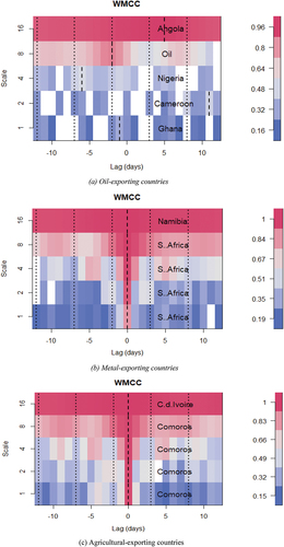
The results indicate that while there is market leadership at some scales for oil-exporting countries, there is no market leadership for metal-exporting countries or agricultural exporting countries. Ghana dominates spillover propagation at the higher scale, and crude oil and Nigeria dominate spillovers at the intermediate scales for oil-exporting countries. For metal-exporting countries, South Africa is the most dominant propagator of spillovers but has no market leadership, followed by Namibia. Comoros dominates spillover propagation, although it has no market leadership, followed by Cote d’Ivoire. The results of the WMCC are therefore quite similar to those of BK18.

5. Conclusion and recommendations

The study focused on the connectedness and contagion between commodity prices and exchange rates in commodity-exporting countries in Sub-Saharan Africa (SSA). The extant literature has concentrated on spillovers among stock markets and commodities in developed and emerging markets, with little emphasis on developing countries like those in SSA. This study concentrated on the returns of commodities and the exchange rate as the origin of contagion and thus emphasised the role of cross-sectional correlation in the origin of connectedness.

In this study, monthly log-return series for crude oil, gold, and cocoa were computed, as were the ERs of five energy-exporting countries, 13 metal-exporting countries, and 13 agricultural-exporting countries. Commodities are used as propagators of spillovers. Spillovers in the system were captured in the static frequency domain (BK18) and the time-varying frequency domain (BK18).

The findings of the study show that there are differences in spillovers and contagion for different commodities. Additionally, when frequency levels rise, connectedness rises as well, and short-lived outbreaks of contagion eventually give way to dependency. The results also revealed that in the medium- to long-term, within-connection levels are lower than in the short-term, so diversification advantages can be realised from both static and time-varying perspectives.

There is no clear evidence from the results of the study that the exchange rates of large commodity-exporting countries are the dominant propagators of spillovers. We also found that gold and cocoa do not dominate spillover transmission to exchange rates in Sub-Saharan Africa, although oil returns and cocoa returns are net transmitters of spillovers to oil-exporting countries and agricultural-exporting countries, respectively. Surprisingly, gold returns happen to be a net receiver of spillovers, with the exchange rates of South Africa, Namibia, and Botswana (all southern African countries) dominating spillover transmission among the metal-exporting countries. Oil returns were dominant among oil-producing countries, while Comoros and Cote d’Ivoire dominated the agricultural-producing countries. Further, Mauritania and Nigeria have a passing contagious association with oil returns in the net’s pairwise directional connectedness. The same can be said for South Africa’s gold returns and the Comoros’ cocoa returns.

Since the study concentrated on contagion and connectedness between commodities and exchange rates, the findings are significant for improving portfolio diversification, risk management, and the stability of the financial market. Policymakers should thus understand and monitor the connection between these markets and their interaction with global shock factors for effective decision-making. Again, instead of focusing on external shocks from commodities, policies aiming to reduce the impact of external shocks on exchange rates should rather be heavy on other commodity-producing countries’ exchange rates. This stems from the fact that shock propagation is stronger in the currency markets of other exporting countries than global commodities. Also, when it comes to how return shocks spread, policymakers should look at the exchange rates of both small and large commodity-producing countries since there is no large country dominance in the study.

From the perspective of investors, there is a need to understand the dynamic connectedness for possible portfolio diversification and hedging strategies. To this end, investors seeking to create a new portfolio can combine investments in gold and the currencies of metal exporting countries due to the weak connection between these assets. Investing in cocoa can also provide a good hedge against the currencies of cocoa exporting countries at low to medium frequencies due to the low shock spillovers from cocoa to those currencies.

In general, this study demonstrates that not only does contagion in the currency market shift or delay, it is also time-frequency dependent. For the energy exporting countries (EEC) and agricultural exporting countries (AEC), decoupling is rejected but partially accepted in the metal exporting countries (MEC). The study has therefore examined the “decoupling hypothesis” in the currency market of CEC in SSA, which was not previously done. This is new evidence that is critical for hedging and risk management decisions, as well as portfolio diversification strategies, for commodity exporting countries that are also commodity dependent. In line with the HMH, policy and investment decisions in SSA’s currency market should take into account the short-, medium-, and long-terms. This is because different factors may affect the movement in each time frame.

Finally, although the shape behaviour of contagion was not described in this study, Owusu Junior et al. (2020) indicated that there is a “shape shift” in contagion among stock markets. By focusing on the higher moment, the strength of contagion between individual commodities and the exchange rate may change, which can also provide an additional source of diversification. As a result, this research can be expanded by comparing contagion at higher levels in commodity-dependent SSA countries.

Data availability statement

Data for the study will be made avialable upon request.

Disclosure statement

No potential conflict of interest was reported by the author(s).

Additional information

Funding

No direct funding was received by the authors for this study.

Appendix A

Figure A1. Plots of Prices and Log-return Series for Commodities

Figure A1. Time series plots of commodity prices and returns.

References

- Adam, M. (2013). Spillovers and contagion in the sovereign CDS market. Bank i Kredyt, 44(6), 571–31. https://bankikredyt.nbp.pl/content/2013/06/bik_06_2013_01_art.pdf
- Agyei, S. K., & Bossman, A. (2023). Exploring the dynamic connectedness between commodities and African equities. Cogent Economics & Finance, 11(1), 2186035. https://doi.org/10.1080/23322039.2023.2186035
- Alagidede, I. P., Boako, G., & Sjo, B. (2021). African equity markets’ exposure to oil and other commodities - implications for global portfolio diversification. Journal of Economics & Finance, 45(2), 288–315. https://doi.org/10.1007/s12197-020-09527-3
- Anas, M., Mujtaba, G., Nayyar, S., & Ashfaq, S. (2020). Time-frequency based dynamics of decoupling or integration between Islamic and conventional equity markets. Journal of Risk and Financial Management, 13(7), 156. https://doi.org/10.3390/jrfm13070156
- Antonakakis, N. (2012). Exchange return Co-movements and volatility spillovers before and after the introduction of euro. Journal of International Financial Markets, Institutions and Money, 22(5), 1091–1109. https://doi.org/10.1016/j.intfin.2012.05.009
- Atenga, E. M., & Mougoué, M. (2021). Return and volatility spillovers to African currencies markets. Journal of International Financial Markets, Institutions and Money, 73, 101348. https://doi.org/10.1016/j.intfin.2021.101348
- Athari, S. A., & Hung, N. T. (2022). Time–frequency return Co-movement among asset classes around the COVID-19 outbreak: Portfolio implications. Journal of Economics & Finance, 46(4), 736–756. https://doi.org/10.1007/s12197-022-09594-8
- Athari, S. A., Kondoz, M., & Kirikkaleli, D. (2021). Dependency between sovereign credit ratings and economic risk: Insight from Balkan countries. Journal of Economics and Business, 116, 105984. https://doi.org/10.1016/j.jeconbus.2021.105984
- Baruník, J., & Křehlík, T. (2018). Measuring the frequency dynamics of financial connectedness and systemic risk. Journal of Financial Econometrics, 16(2), 271–296. https://doi.org/10.1093/jjfinec/nby001
- Baur, D. G., & Lucey, B. M. (2010). Is gold a hedge or a safe haven? An analysis of stocks, bonds and gold. Financial Review, 45(2), 217–229. https://doi.org/10.1111/j.1540-6288.2010.00244.x
- Bekaert, G., Campbell, R. H., & Ng, A. (2005). Market integration and contagion. The Journal of Business, 78(1), 39–69. https://doi.org/10.1086/426519
- Benhmad, F. (2012). Modeling nonlinear Granger causality between the oil price and U.S. dollar: A wavelet based approach. Economic Modelling, 29(4), 1505–1514. https://doi.org/10.1016/j.econmod.2012.01.003
- Boako, G., & Alagidede, P. (2017). Examining evidence of ‘shift-contagion’ in African stock markets: A covar-copula approach. Review of Development Finance, 7(2), 142–156. https://doi.org/10.1016/j.rdf.2017.09.001
- Bouri, E., Jain, A., Biswal, P., & Roubaud, D. (2017). Cointegration and nonlinear causality amongst gold, oil, and the Indian stock market: Evidence from implied volatility indices. Resources Policy, 52, 201–206. https://doi.org/10.1016/j.resourpol.2017.03.003
- Bubák, V., Kočenda, E., & Žikeš, F. (2011). Volatility transmission in emerging European foreign exchange markets. Journal of Banking & Finance, 35(11), 2829–2841. https://doi.org/10.1016/j.jbankfin.2011.03.012
- Caporin, M., Pelizzon, L., Ravazzolo, F., & Rigobon, R. (2018). Measuring sovereign contagion in Europe. Journal of Financial Stability, 34, 150–181. https://doi.org/10.1016/j.jfs.2017.12.004
- Ciner, C., Gurdgiev, C., & Lucey, B. M. (2013). Hedges and safe havens: An examination of stocks, bonds, gold, oil and exchange rates. International Review of Financial Analysis, 29, 202–211. https://doi.org/10.1016/j.irfa.2012.12.001
- Dai, X., Wang, Q., Zha, D., & Zhou, D. (2020). Multi-scale dependence structure and risk contagion between oil, gold, and US exchange rate: A wavelet-based vine-copula approach. Energy Economics, 88, 104774. https://doi.org/10.1016/j.eneco.2020.104774
- Dickey, D. A., & Fuller, W. A. (1979). Distribution of the estimators for autoregressive time series with a unit root. Journal of the American Statistical Association, 74(366), 427. https://doi.org/10.2307/2286348
- Diebold, F. X., & Yilmaz, K. (2009). Measuring financial asset return and volatility spillovers, with application to global equity markets. The Economic Journal, 119(534), 158–171. https://doi.org/10.1111/j.1468-0297.2008.02208.x
- Diebold, F. X., & Yilmaz, K. (2012). Better to give than to receive: Predictive directional measurement of volatility spillovers. International Journal of Forecasting, 28(1), 57{66. https://doi.org/10.1016/j.ijforecast.2011.02.006
- Diebold, F. X., & Yilmaz, K. (2014). On the network topology of variance decompositions: Measuring the connectedness of financial frms. Journal of Econometrics, 182(1), 119–134. https://doi.org/10.1016/j.jeconom.2014.04.012
- Dornbusch, R., Park, Y. C., & Claessen, S. (2000). Contagion: understanding how it spreads. The World Bank Research Observer, 15(2), 177–197. https://doi.org/10.1093/wbro/15.2.177
- Fernández-Macho J. (2012). Wavelet multiple correlation and cross-correlation: A multiscale analysis of Eurozone stock markets. Physica A: Statistical Mechanics and its Applications, 391(4), 1097–1104. 10.1016/j.physa.2011.11.002
- Forbes, K. J., & Rigobon, R. (2002). No contagion, only interdependence: Measuring stock market Comovements. The Journal of Finance, 57(5), 2223–2261. https://doi.org/10.1111/0022-1082.00494
- Gulko, L. (2002). Decoupling. The Journal of Portfolio Management, 28(3), 59–66. https://doi.org/10.3905/jpm.2002.319843
- Huynh, T. L., Nasir, M. A., & Nguyen, D. K. (2020). Spillovers and connectedness in foreign exchange markets: The role of trade policy uncertainty. The Quarterly Review of Economics & Finance. https://doi.org/10.1016/j.qref.2020.09.001
- Jiang, Z., Arreola Hernandez, J., McIver, R. P., & Yoon, S. (2022). Nonlinear dependence and spillovers between currency markets and global financial market variables. Systems. https://doi.org/10.20944/preprints202205.0265.v1
- Ji, Q., & Fan, Y. (2012). How does oil price volatility affect non-energy commodity markets? Applied Energy, 89(1), 273–280. https://doi.org/10.1016/j.apenergy.2011.07.038
- Kaminsky, G. L., Reinhart, C. M., & Végh, C. A. (2003). The unholy trinity of financial contagion. Journal of Economic Perspectives, 17(4), 51–74. https://doi.org/10.1257/089533003772034899
- Katusiime, L. (2018). Investigating spillover effects between foreign exchange rate volatility and commodity price volatility in Uganda. Economies, 7(1), 1. https://doi.org/10.3390/economies7010001
- Kirikkaleli, D., & Athari, S. A. (2020). Time-frequency Co-movements between bank credit supply and economic growth in an emerging market: Does the bank ownership structure matter? The North American Journal of Economics & Finance, 54, 101239. https://doi.org/10.1016/j.najef.2020.101239
- Kočenda, E., & Moravcová, M. (2019). Exchange rate comovements, hedging and volatility spillovers on new EU forex markets. Journal of International Financial Markets, Institutions and Money, 58, 42–64. https://doi.org/10.1016/j.intfin.2018.09.009
- Kose, M., Otrok, C., & Prasad, E. S. (2008). Global Business Cycles: Convergence or Decoupling? NBER Working Paper No. 14292.
- Kose, M., & Prasad, E. S. (2010). Emerging markets: Resilience and growth amid global turmoil. Brookings Institution Press.
- Lin, C. (2012). The comovement between exchange rates and stock prices in the Asian emerging markets. International Review of Economics & Finance, 22(1), 161–172. https://doi.org/10.1016/j.iref.2011.09.006
- Lo, A. W. (2004). The adaptive markets hypothesis. The Journal of Portfolio Management, 30(5), 15–29. https://doi.org/10.3905/jpm.2004.442611
- Maund, C. (2007, April 1). The gold bull market remembers how Gordon Brown sold half of Britain reserves at the lowest price. The Market Oracle. http://www.marketoracle.co.uk/Article670.html
- Moore, T., & Wang, P. (2014). Dynamic linkage between real exchange rates and stock prices: Evidence from developed and emerging Asian markets. International Review of Economics & Finance, 29, 1–11. https://doi.org/10.1016/j.iref.2013.02.004
- Muller, U. A., Dacorogna, M. M., Dav´e, R. D., Pictet, O. V., Olsen, R. B., & Ward, J. R. (1993). Fractals and intrinsic time: A challenge to econometricians. In Unpoblished Manuscript, Olsen & Associate, Zurich, (p. 130). O&A Research Group.
- Nyang`oro Owen, (2017). “Working Paper 285 - capital inflows and economic growth in Sub-Saharan Africa,” Working Paper Series 2409, African Development Bank.
- Owusu Junior, P., Alagidede, I., & Tweneboah, G. (2020). Shape-shift contagion in emerging markets equities: Evidence from frequency- and time-domain analysis. Economics & Business Letters, 9(3), 146–156. https://doi.org/10.17811/ebl.9.3.2020.146-156
- Owusu Junior, P., & Gherghina, S. C. (2022). Dynamic connectedness, spillovers, and delayed contagion between Islamic and conventional bond markets: Time- and frequency-domain approach in COVID-19 era. Discrete Dynamics in Nature and Society, 2022, 1–18. https://doi.org/10.1155/2022/1606314
- Phillips, P. C., & Perron, P. (1988). Testing for a unit root in time series regression. Biometrika, 75(2), 335–346. https://doi.org/10.1093/biomet/75.2.335
- Polanco-Martínez, J. M. (2019). Dynamic relationship analysis between NAFTA stock markets using nonlinear, nonparametric, non-stationary methods. Nonlinear Dynamics, 97(1), 369–389. https://doi.org/10.1007/s11071-019-04974-y
- Polanco-Martínez, J., Fernández-Macho, J., Neumann, M., & Faria, S. (2018). A pre-crisis vs. crisis analysis of peripheral EU stock markets by means of wavelet transform and a nonlinear causality test. Physica A: Statistical Mechanics and Its Applications, 490, 1211–1227. https://doi.org/10.1016/j.physa.2017.08.065
- Pritsker, M. (2000). The channels of Contagion. The Contagion Conference, Available at: siteresources.worldbank.org/INTMACRO/Resources.
- Reboredo, J. C., & Rivera-Castro, M. A. (2013). A wavelet decomposition approach to crude oil price and exchange rate dependence. Economic Modelling, 32, 42–57. https://doi.org/10.1016/j.econmod.2012.12.028
- Reboredo, J. C., & Rivera-Castro, M. A. (2014). Can gold hedge and preserve value when the US dollar depreciates? Economic Modelling, 39, 168–173. https://doi.org/10.1016/j.econmod.2014.02.038
- Saiti, B., Bacha, O. I., & Masih, M. (2015). Testing the conventional and Islamic financial market contagion: Evidence from wavelet analysis. Emerging Markets Finance and Trade, 52(8), 1832–1849. https://doi.org/10.1080/1540496x.2015.1087784
- Salisu, A. A., Oyewole, O. J., & Fasanya, I. O. (2018). Modelling return and volatility spillovers in global foreign exchange markets. Journal of Information and Optimization Sciences, 39(7), 1417–1448. https://doi.org/10.1080/02522667.2017.1367507
- Shen, H., Pan, Q., Zhao, L., & Ng, P. (2022). Risk contagion between global commodities from the perspective of volatility spillover. Energies, 15(7), 2492. https://doi.org/10.3390/en15072492
- Tiwari, A. K., Trabelsi, N., Alqahtani, F., & Bachmeier, L. (2019). Modelling systemic risk and dependence structure between the prices of crude oil and exchange rates in BRICS economies: Evidence using quantile coherency and NGCoVaR approaches. Energy Economics, 81(C), 1011–1028. https://doi.org/10.1016/j.eneco.2019.06.008
- United Nations Conference on Trade and Development. (2021) . State of commodity dependence 2021. United Nations.
- Wen, F., Xiao, J., Huang, C., & Xia, X. (2017). Interaction between oil and US dollar exchange rate: Nonlinear causality, time-varying influence and structural breaks in volatility. Applied Economics, 50(3), 319–334. https://doi.org/10.1080/00036846.2017.1321838
- World Bank Group. (2018). Migration and Remittances, April 2018: Recent Developments and Outlook. https://doi.org/10.1596/30280
- World Economic Outlook. (2007). Spillovers and cycles in the global economy. IMF.
- Yıldırım, D. Ç., Erdoğan, F., & Tarı, E. N. (2022). Time-varying volatility spillovers between real exchange rate and real commodity prices for emerging market economies. Resources Policy, 76, 102586. https://doi.org/10.1016/j.resourpol.2022.102586
- Yilmaz, K. (2010). Return and volatility spillovers among the East Asian equity markets. Journal of Asian Economics, 21(3), 304–313. https://doi.org/10.1016/j.asieco.2009.09.001