The effects of sales surprise on inventory turnover: An empirical study

Abstract

Sales surprise (SS) is a significant factor in a firm’s inventory turnover (ITO). In order to estimate SS, it is necessary to select an appropriate approach of sales forecasting. The current study’s main purpose is to examine the effects of SS on ITO. The data was gained from the Albertina database from 2017 to 2021, for two sectors: manufacturing and construction. The Czech firms’ panel data was used to estimate sales forecasts by four different methods: (i) sales linear forecast (SLF), (ii) sales change (SCH), (iii) sales growth (SG), and (iv) sales forecast random walk (SRW). The two most accurate methods were chosen to calculate SS: sales surprise linear forecast (SSLF) and sales surprise random walk (SSRW). After estimating four different regression models by employing the fixed-effect panel model, the results show that SSRW is positively correlated with ITO. The sales surprise linear forecast (SSLF) is found to be insignificant. Capital intensity (CI) has a positive impact on ITO; on the other hand, the relationship between gross margin (GMN) and ITO is negative. This is the first research in which SS is measured by four different techniques, and then the two most accurate techniques are used to examine the effects of SS on ITO. Therefore, the findings of the current research will be fruitful for managers, academics, policymakers, and directors of firms to estimate SS using different techniques and to understand the effects of SS on ITO. Hence, the research will be useful to the firms’ management in many contexts.

Keywords:

• inventory turnover
• sales surprise
• sales forecast
• Czech firms
• fixed-effect model

JEL classification:

• G17
• G31
• L60

1. Introduction

Kolias et al. (2011) argued that inventory is considered an asset that is difficult to manage. The most frequently used measure of inventory management performance is inventory turnover (ITO) (Breivik, 2019). ITO denotes the relationship between the cost of goods sold and the average inventory level of a firm. ITO is a conventional measure employed to gauge inventory productivity at the firm-level, and it measures the frequency at which a firm converts its inventory within a specified timeframe, typically a year. Mahajan et al. (2023) argued that ITO is often used to measure a firm’s performance. Sales surprise (SS) is the ratio of actual sales to forecast sales for a given period. SS is an important determinant of firms’ ITO. Previous literature identified variables such as gross margin (GMN), capital intensity (CI), and SS that might be correlated with ITO (Gaur et al., 2005; Sano & Yamada, 2020). According to Sano and Yamada (2020), SS is a crucial determinant of a firm’s ITO. Therefore, it is important to choose an accurate method of forecasting sales in order to estimate SS.

Breivik (2019) argued that the research on inventory performance in previous literature can be divided into two types. The first type treats inventory performance and examines inventory performance factors such as ITO, inventory in levels, and in days. This approach can be augmented by numerous macroeconomic indicators, such as the purchase manager index, gross domestic product, or interest rate (Chen et al., 2005, 2007). Some authors also adjusted by some determinants of inventory, such as CI, GMN, sales growth, etc (Breivik, 2019; Breivik et al., 2023; Gaur & Kesavan, 2015; Kwak, 2019; Na et al., 2021; Sano & Yamada, 2020; Wan et al., 2020). The second type is concerned with how inventory performance affects financial performance (Alan et al., 2014; Capkun et al., 2009; Hashed & Shaik, 2022; Isaksson & Seifert, 2014; Kesavan & Mani, 2013; Park & Kim, 2020; Shockley & Turner, 2014). Garba et al. (2020) claimed that there is limited literature globally that investigates the role of inventory management on profitability.

Gaur et al. (2005) and Sano and Yamada (2020) proposed that ITO is driven by three factors: GMN, CI, and SS. The scholars demonstrated that these factors have strong explanatory power regarding ITO. The scholars suggested that ITO should not be used by itself for managerial decision-making and performance analysis. Gaur et al. (2005) used 311 U.S. retail firms’ data for the years from 1985 to 2000. The findings revealed that GMN has a negative impact on ITO. Conversely, CI and SS have a positive impact on ITO. Sano and Yamada (2020) used the data of 1,291 Japanese manufacturing and retail firms for the years 1997 to 2014. The researchers utilized various approaches, including Holt’s technique and management prediction, to quantify SS. The researchers discovered an unfavorable correlation between GMN and ITO, along with a favorable influence of CI and SS on ITO.

Numerous scholars have expanded upon the research conducted by Gaur et al. (2005) by scrutinizing varied industries and countries. For example, Kolias et al. (2011) conducted an analysis of the fiscal data of 566 Greek retail firms spanning from 2000 to 2005. They arrived at identical outcomes, where GMN has an adverse effect on ITO while CI and SS have a favorable effect on ITO. Gaur and Kesavan (2015) evaluated the effects of sales growth rate and firm size utilizing data from 353 U.S. retail firms from 1985 to 2003. Their study evinced that ITO exhibits a positive correlation with sales growth rate and firm size.

The research by Gaur et al. (2005) focused on the retail sector, and the research by Sano and Yamada (2020) focused on the manufacturing and retail sectors. Various studies have focused on the manufacturing sector (Alnaim & Kouaib, 2023; Capkun et al., 2009; Kwak, 2019; Truong, 2023). In the current study, the firms are chosen from two sectors: manufacturing and construction. The two sectors were selected for four reasons. (i) Both sectors have the same characteristics, such as high operating risk, a lengthy development cycle, high investment, etc. (ii) It is logical to focus on the sectors, as ITO and SS are relevant to the sectors. (iii) The sectors are both labour and capital intensive. (iv) The sectors have a substantial share of Czechia’s GDP.

The main aim of the current study is to examine the effects of SS on ITO. This study differs from earlier research in that it uses four different methodologies to examine sales forecasts. After careful analysis, the two most accurate sales forecast methods are employed: sales surprise linear forecast (SSLF) and sales surprise random walk (SSRW). Then the impacts of SSLF and SSRW on ITO are examined individually. Therefore, four regression models were run to investigate the comprehensive empirical relationship between SS and ITO. There are a few studies on ITO, but not much is known about the Czech firm’s ITO and SS. The current research fills these gaps. Hence, the study will contribute to the literature and practical knowledge in many contexts.

Following the introduction section, the rest of the paper is organized as follows: Section 2 presents a literature review related to ITO. Section 3 defines the performance variables and presents the methodology. Section 4 synthesizes the empirical models used in estimation. Section 5 is about the discussion of the empirical results. The last section discusses the findings, managerial implications, and limitations of the study. Moreover, this section also gives guidelines for future research.

2. Literature review

In the previous literature, scholars have directed their attention towards evaluating the ramifications of diverse distribution (or production) systems and initiatives on inventory performance at the firm-level by using mathematical inventory models. Certain scholars have also delved into the assessment of inventory performance at the industry level and conducted empirical research aimed at determining whether firms enhance their inventory management practices (Chen et al., 2005, 2007; Rajagopalan & Malhotra, 2001). A number of studies have concentrated on comprehending how inventory performance correlates with financial outperformance in the stock market (Capkun et al., 2009; Gaur et al., 2014). Various authors have endeavored to explicate the differences in inventory performance and account for a plethora of factors that have an impact on ITO (Gaur et al., 2005; Saprudin et al., 2022). These factors, such as scale economies, SS, product variety, GMN, number of locations, and CI, are of utmost importance to investigate in order to appropriately benchmark the inventory performance of a firm against other firms within the same industry. The majority of authors have employed the ITO ratio as a measure of the inventory performance of a firm in their empirical studies on inventory management.

Rajagopalan and Malhotra (2001) studied aggregate industry-level data for 20 industrial sectors of the United States (U.S.) manufacturers’ inventory turns to explore whether the inventory turns have declined with time for each inventory type: finished goods, work-in-process, and raw materials. They took the data from 1961 to 1994 and found that six sectors show an increasing trend in inventory turns for finished goods. However, work-in-process inventory did not show a better improvement than finished goods inventory during the study period. Capkun et al. (2009) studied the relationship between the performance of inventory components and the financial performance of US manufacturing firms from 1980 to 2005. The study found a positive correlation between the variables. Breivik et al. (2023) investigated how firm size, time trends, and environmental factors are correlated to inventory performance. By using 16 years of demographic data and financial accounting data of Norwegian small and medium-sized enterprises (SMEs) home improvement retailers, the authors employed a stochastic frontier model to explore how ITO is linked to productivity and efficiency. The scholars allowed the model to control for some variables such as sales growth, firm size, GMN, and CI. The authors explored how efficiency in inventory performance varies depending on store location and local market conditions. Furthermore, the scholar found a positive relationship between firm inventory efficiency and firm size.

Hançerlioğulları et al. (2016) studied the effect of different measures on inventory performance by using regression analysis. The scholars used the financial data of 304 U.S. retail firms from 1985 to 2009. The results indicate that ITO is negatively correlated with GMN and positively correlated with CI and SS. Lee et al. (2015) investigated the relationship between the firm’s innovation performance and ITO performance by employing non-service U.S. public firms’ data from 1976 to 2005. The findings of the study revealed that there is a positive correlation between ITO and innovation performance. Shan and Zhu (2013) undertook an analysis of the inventory performance of 1,286 Chinese firms through the development of an empirical model. The results of the study revealed a significant decrease in inventory levels over time. The findings are consistent with prior research conducted in the U.S.

The relationship between inventory performance and firms’ financial performance has been explored by many authors (Alnaim & Kouaib, 2023; Atnafu et al., 2018; Elsayed, 2015; Eroglu & Hofer, 2014; Hashed & Shaik, 2022; Koumanakos, 2008; Obermaier & Donhauser, 2012; Sekeroglu & Altan, 2014; Truong, 2023). These scholars reported a positive relationship between firms’ financial performance and inventory performance. For instance, a study conducted by Kasim and Antwi (2015) examined the relationship between inventory management and firm performance. The authors investigated the effect of inventory management on financial performance by using the primary data of 300 SMEs in the northern region of Ghana. The study found that firms that manage inventory well improve their financial performance. Similar results were reported by Orobia et al. (2020) by using the data of 304 small business firms in Uganda. A study by Alan et al. (2014) also reported a positive relationship between stock price and inventory productivity.

Most of the previous research showed that ITO is positively linked to financial performance, which means that firms improve financial performance by increasing their efforts to enhance ITO. Alrjoub and Ahmad (2017) argued that most of the empirical studies explored the relationship between total inventories and firm performance. There are only a few studies that have considered the effect of inventory types on firm performance (Capkun et al., 2009; Eroglu & Hofer, 2011). Moreover, in some studies, the scholars found conflicting results. For example, Rumyantsev and Netessine (2007a) studied manufacturing businesses across eight countries and reported a negative relationship between profitability and days of finished-goods inventory. Nasution (2020) found that ITO does not have a positive effect on firm performance in automotive firms that are listed on the Indonesia Stock Exchange. In the same way, Capkun et al. (2009) explored a negative relationship between sales and levels of raw material inventory, work-in-progress inventory, and finished-goods inventory. The scholars concluded that the finished-goods inventory was the most important inventory. On the other hand, Rumyantsev and Netessine (2007b) and Cannon (2008) examined no relationship between financial performance and inventory. According to Eroglu and Hofer (2011), these findings might be subject to data issues and poor modelling.

From the above discussion, it is clear that most of the former studies (where most of the studies were conducted in the U.S., Japan, and European countries) revealed the relationship between inventory performance (or inventory management) and organizational performance; inventory productivity and stock price; and ITO and SS. Due to conflicting findings in the previous literature, there is room to investigate the impacts of SS on ITO. Moreover, the current study is different from the earlier studies for the following reasons: (i) SS was estimated by one method in the study by Gaur et al. (2005), and SS was estimated by two different methods by Sano and Yamada (2020). However, in the current study, four methods are used to measure SS, and then two precise methods are employed in regression models: sales surprise linear forecast (SSLF) and sales surprise random walk (SSRW). (ii) To the best of our knowledge, this is the first study using Czech firms’ data to explore the impact of SS on ITO. (iii) The study by Gaur et al. (2005) is based on the retail sector, and the research by Sano and Yamada (2020) is based on two sectors: retail and manufacturing. The current study provides empirical evidence, particularly in the fields of construction and manufacturing. These particular sectors were chosen in the study due to the availability of data and their crucial role in the economy of the Czech Republic. Based on statistical figures from the World Bank, the manufacturing industry contributed 22.38% to the gross domestic product of the Czech Republic in the year 2021, while the construction sector accounted for 5.7%.

3. Methodology

3.1. Source of data

The Albertina database was utilized to retrieve secondary data of Czech firms between the years 2017 to 2021. As highlighted by Chandrapala and Knápková (2013), the Albertina database encompasses the expansion, processing, and distribution of databases that cater to the ever-evolving free-market environment in the Czech Republic. Additionally, Činčalová and Hedija (2020) posit that the Albertina database comprises of data pertaining to more than 2.7 million subjects. Numerous authors have used the secondary data from the Albertina database in recent studies, such as Lososová and Zdeněk (2023); Yousaf (2023b); Dvořáková and Vacek (2023); Yousaf (2023a); Heinzová et al. (2023); Yousaf (2022); Dokulil et al. (2022); Yousaf and Bris (2021); Yousaf et al. (2021); Vrbka (2020). The sample of the study took 341 Czech firms. The unbalanced panel data sample is chosen randomly from two sectors: construction and manufacturing.

3.2. Sales forecast

Sales forecasts are essential for both external and internal decision-makers. External decision-makers must often rely on limited information, particularly from competitors and industry peers. This section compares four methods that rely on limited information, annual sales for only four years. The annual data is used because quarterly data is often unavailable, particularly in smaller countries and in countries with a limited history of disclosure. This is particularly true for countries with poorly developed capital markets, where companies are privately or closely held and required to disclose limited information to the public. Therefore, the data covers only a short time period, 2017–2021, as the data was available for only five years from the Albertina database. Hence, five years of data were used to demonstrate each method’s ability to forecast sales in a limited information environment.

The sample period was divided into two groups: the first three years (2017–2019) are used as the model training period, where four different methods estimated sales forecasts, and the last two years (2020–2021) form the model test period, where four different models were estimated by panel fixed effect. The studies by Gaur et al. (2005) and Sano and Yamada (2020) employed Holt’s method to estimate SS. Holt’s method requires quarterly data and a longer time period. In the present study, annual data with a short time period is used. Due to the short time series, each method uses a linear model to forecast sales beyond the fourth year. The first method, sales linear forecast (SLF), uses the linear trend in the level of sales (x) for a given year:

(1) $a=\bar{y}-b\bar{x}$(1)

where

(2) $b={\displaystyle \sum \left(x-\overline{x}\right)}\left(y-\overline{y}\right)\sum {(x-\overline{x})}^2$(2)

The second method, sales change (SCH), uses the linear trend in the change in sales (Δx) for a given year:

(3) $a=\overline{y}-b\stackrel{-}{\Delta x}$(3)

where

(4) $\mathrm{\Delta }\mathrm{x}=\mathrm{S}\mathrm{a}\mathrm{l}\mathrm{e}{\mathrm{s}}_{\mathrm{t}}-\mathrm{S}\mathrm{a}\mathrm{l}\mathrm{e}{\mathrm{s}}_{\mathrm{t}-1}$(4)

and

(5) $b=\sum (\Delta x-\stackrel{-}{\Delta x}\left(y-\overline{y}\right)\sum {(\overline{x}-\stackrel{-}{\Delta x})}^2$(5)

The forecast of the change in sales is added to sales in year four to achieve the sales forecast for year five.

The third method, sales growth (SG), uses the linear trend in the rate of change in sales (ẋ) for a given year (y):

(6) $a=\overline{y}-b\overline{\dot{x}}$(6)

where

(7) $\overline{\dot{x}}=\frac{Sale{s}_t-Sale{s}_{t-1}}{Sale{s}_{t-1}}$(7)

and

(8) $b=\sum (\dot{x}-\overline{\dot{x}}\left(y-\overline{y}\right)\sum {(\dot{x}-\overline{\dot{x}})}^2$(8)

The forecast of the percentage change in sales is multiplied by year four sales, and the product is added to sales in year four to achieve the sales forecast for year five.

The last method, sales forecast random walk (SRW), assumes that sales follow a random walk (Hyndman & Koehler, 2006). Therefore, the sales forecast for year five is year four sales.

Each method was applied to all firms in the sample. The mean and median absolute forecast errors were chosen to select the best sales forecast methods. The absolute forecast error was calculated as the absolute value of the difference between actual sales in year five minus the year five sales forecast. Table 1 compares the mean and median absolute error rates between the four methods.

Table 1. Absolute error rates (source: authors)

	Mean	Median	Std. Dev.	Freq.
Abs(ESLF)	0.142	0.103	0.137	1022
Abs(ESCH)	0.183	0.125	0.179	1016
Abs(ESG)	0.206	0.160	0.194	995
Abs(ESRW)	0.113	0.071	0.130	1002
Average	0.161	0.114	0.160	998

where:

ESLF = Sales_t = 5 – SLF_t = 5

ESCH = Sales_t = 5 – SCH_t = 5

ESG = Sales_t = 5 – SG_t = 5

ESRW = Sales_t = 5 – SRW_t = 5

As shown in Table 1, the random walk method produced the lowest mean and median absolute forecast errors. The linear forecast of sales was the second-best, followed by forecasting a linear trend in the change in sales. The worst forecasting method was forecasting a linear trend in the sales growth rate. One-way ANOVA showed a significant overall difference between group means (p = .000). Bonferroni post hoc tests revealed that there is a significant difference between Abs(ESLF) and Abs(ESG) (p = .029); between Abs(ESCH) and Abs(ESRW), (p = .015); and between Abs(ESG) Abs(ESRW) (p = .000).¹

Due to the overall effectiveness of the sales forecast random walk (SRW) and the sales linear forecast (SLF), these two methods were chosen to calculate SS in the empirical tests.

3.3. Model variables

ITO (inventory turnover) is the dependent variable in the current study. GMN (gross margin), CI (capital intensity), SSRW (sales surprise random walk), and SSLF (sales surprise linear forecast) are independent variables. YEARDUM is a year dummy variable; the value of YEARDUM for 2021 will be one; otherwise, its value will be zero.

ITO in year t of firm i is defined as below:

(9) $IT{O}_{it}=\frac{COG{S}_{it}}{IN{V}_{it}}$(9)

Where ITO_it = inventory turnover, COGS_it = cost of goods sold, and INV_it = average inventory in acquired value of firm i in year t.

(10) $GM{N}_{it}=Sale{s}_{it}-COG{S}_{it}Sale{s}_{it}$(10)

Where GMN_it = Gross margin, Sales_it = total revenue of firm i in year t.

Previous literature showed that GMN is negatively correlated with ITO. According to Sano and Yamada (2020), high GMN indicates a high unit underage cost and raises the optimal order quantity, so the value of ITO decreases. Gaur et al. (2005) argue that a higher value of GMN indirectly reduces ITO through product variety, price, and the length of the product life cycle.

(11) $C{I}_{it}=\hspace{0.17em}\frac{GF{A}_{it}}{(IN{V}_{it}+GF{A}_{it})}\hspace{0.17em}$(11)

CI_it = Capital intensity, GFA_it = gross fixed assets, consisting of the sum of property, land, equipment of firm i in year t.

CI captures the degree of investments invested in fixed assets, and these investments expand inventory management efficiency. So, there is a positive relationship between CI and ITO.

Following Sano and Yamada (2020), sales surprise random walk (SSRW), or sales surprise linear forecast (SSLF) of firm i in year t is defined as follows:

(12) $SSL{F}_{it}=\left(Sale{s}_{it}\right)/\left(SL{F}_{it}\right)$(12)

SSLF_it is firm i’s sales linear forecast of sales in year t.

(13) $SSR{W}_{it}=\left(Sale{s}_{it}\right)/\left(SR{W}_{it}\right)$(13)

Where SSRW_it is firm i’s sales random walk forecast of sales in year t.

3.4. Model specification

Following Sano and Yamada (2020); and Gaur et al. (2005), the log-values of all variables are used to estimate the log-linear models. The lagged values of the dependent variable (ITO) are employed as explanatory variables as it is most likely that the present value depends on its past values (i.e., autocorrelated). Hence, the regression equations are given below.

$ln\left(\left(IT{O}_{it}\right)=\alpha +{\beta }_{1}ln\left(GM{N}_{it}\right)+{\beta }_{2}ln\left(C{I}_{it}\right)+{\beta }_{3}ln\left(SSL{F}_{it}\right)+{\beta }_4\left(YEARDU{M}_{it}\right)+{\eta }_i+{\epsilon }_{it}\right)$

Model 1

$\ln \left(IT{O}_{it}\right)=\alpha +{\beta }_1\ln \left(GM{N}_{it}\right)+{\beta }_2\ln \left(CI\right)+{\beta }_3\ln \left(SSL{F}_{it}\right)+{\beta }_4\left(YEARDU{M}_{it}\right)+{\beta }_5\ln \left(\left(ITOlag\right)+{\eta }_i+{\epsilon }_{it}\right)$

Model 2

$ln\left(\left(IT{O}_{it}\right)=\alpha +{\beta }_{1}ln\left(GM{N}_{it}\right)+{\beta }_{2}ln\left(C{I}_{it}\right)+{\beta }_{3}ln\left(SSR{W}_{it}\right)+{\beta }_4\left(YEARDU{M}_{it}\right)+{\eta }_i+{\epsilon }_{it}\right)$

Model 3

$\ln \left(IT{O}_{it}\right)=\alpha +{\beta }_1\ln \left(GM{N}_{it}\right)+{\beta }_2\ln \left(C{I}_{it}\right)+{\beta }_3\ln \left(SSR{W}_{it}\right)+{\beta }_4\left(YEARDU{M}_{it}\right)+{\beta }_5\ln \left(\left(ITOla{g}_{it}\right)+{\eta }_i+{\epsilon }_{it}\right)$

Model 4

From Model 1 to Model 4, α is the intercept, β values are the regression coefficients of the independent variables. i = 1, 2, 3, …, n is the number of firms, t is time; ƞ_i and ε_it are the unobserved firm-specific effects and error term for firm i at time t, respectively.

4. Empirical results

The statistical characteristics of all chosen variables have been laid out in Table 2. The calculations were executed utilizing the STATA 16.0 software.

Table 2. Descriptive statistics of the chosen variables

stats	lnITO	lnGMN	lnCI	lnSSLF	lnSSRW	lnITOlag	YEARDUM
Mean	1.188	−1.024	−0.523	−0.051	0.050	1.208	0.5
Median	1.204	−0.970	−0.446	0.010	0.027	1.235	0.5
Min	−0.471	−1.802	−1.952	−10.731	−1.051	−0.414	0
Max	2.614	−0.350	−0.080	2.002	2.019	2.614	1
S.D.	0.553	0.296	0.336	1.023	0.300	0.554	0.501
Skewness	−0.210	−0.403	−1.733	−8.520	2.789	−0.218	0
Kurtosis	3.084	2.652	6.779	84.666	22.308	3.161	1
N	676	660	672	670	672	674	676

The mean and standard deviation of lnITO are 1.188 and 0.553, respectively. Among the chosen variables, the mean and median values appear to be nearly identical. Nevertheless, the mean and standard deviation values of lnSSRW and lnSSLF exhibit slight differences. Skewness pertains to the direction and magnitude of the skew, with a skewness value of zero indicating perfectly symmetrical data. It is improbable for real-world data to possess a skewness value of zero, as this is reserved for the normal distribution. Kurtosis, on the other hand, describes the height and sharpness of the central peak relative to a standard bell curve. A kurtosis value that is negative denotes a light-tailed distribution, while a positive value indicates a heavy-tailed distribution. The standard normal distribution is expected to have a kurtosis value of zero in many textbooks. Nevertheless, Malhotra and Dash (2016) recommend a range of ± 1 for skewness and ± 3 for kurtosis. In contrast, Simon et al. (2017) argue that skewness and kurtosis should fall within the ranges of ± 3 and ± 10, respectively. Most of the selected variables in Table 2 exhibit a normal distribution, as evidenced by their skewness and kurtosis values.

Table 3 illustrates the correlation coefficients of the selected variables. lnITO has a negative correlation with lnGMN, lnSSLF, and YEARDUM, but ITO is positively correlated with lnCI, lnSSRW, and lnITOlag. lnSSLF is negatively correlated with lnCI. Table 3 also reports the variance inflation factor (VIF) coefficients. The VIF is used to address the problem of multicollinearity in the sample. According to Nachane (2006), multicollinearity is a serious problem if the value of the VIF is more than 10. It seems that there is no multicollinearity in the variables of the current study, as all values of VIF in Table 3 are lower than 10.

Table 3. Correlation coefficient

	lnITO	lnGMN	lnCI	lnSSLF	lnSSRW	lnITOlag	YEARDUM	VIF
lnITO	1
lnGMN	−0.236*	1						1.16
lnCI	0.443*	0.117	1					1.28
lnSSLF	−0.019	0.051	−0.032	1				1.03
lnSSRW	0.157*	0.031	0.07	−0.006	1			1.02
lnITOlag	0.931*	−0.269*	0.404*	−0.065	0.054	1		1.37
YEARDUM	−0.008	0.022	0.009	−0.145*	−0.103	−0.028	1	1.04

Note: *denote p < 0.05.

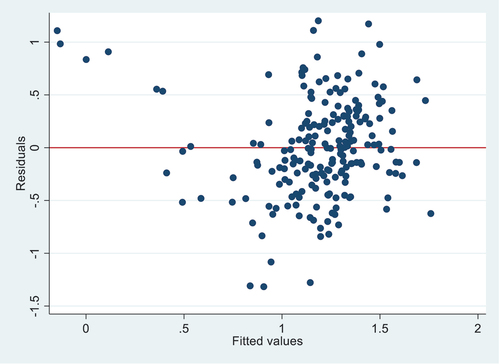
To ensure the validity of the regression results, the heteroskedasticity of the data is checked. It is clear from Figure 1 that the data is free from heteroskedasticity, as there is no pattern or clustering in the data.²

Figure 1. Robustness test for Model 1.

Before running the regression, the stationarity of the variables is also checked by the Fisher type unit-root test. The following hypotheses are formulated to check the unit-roots in the data:

Ho: All panels are stationary

Ha: Some panels contain unit roots

The results revealed that all the selected variables are stationary, as the p-values of the variables are greater than the significance level (0.05).³ Therefore, it is appropriate to run the regression and estimate the Models (from Model 1 to Model 4). There are many different panel data models that can be used in the current empirical study. However, the fixed effect model is used in the study to examine the effects of SS on ITO due to two reasons: (i) After employing the Hausman test, the results revealed that the fixed effects model should be preferred to the random effect model. (ii) Various authors have used the fixed effect model in the most recent studies.

A panel fixed effect model estimates individual differences in intercepts, assuming the constant slopes and constant variance across individuals, where the fixed effects are tested by the F test (Breusch & Pagan, 1980). Various authors employed the panel fixed effect model in their research by considering ITO as a dependent variable (Alnaim & Kouaib, 2023; Gaur & Kesavan, 2015; Gaur et al., 2005; Na et al., 2021; Sano & Yamada, 2020). Many studies also used the fixed-effect model even though the dependent variable was not ITO (Abe et al., 2021; Rangkuti, 2020; Xiang et al., 2021). The fixed effect model is very relevant; therefore, the model is also employed in this research. The results are presented in Table 4.

Table 4. Results of the fixed-effect model

	Model 1	Model 2	Model 3	Model 4
lnGMN	−0.144 (0.088)	−0.175*** (0.084)	−0.288*** (0.084)	−0.281*** (0.084)
lnCI	0.968*** (0.174)	0.942*** (0.165)	1.082*** (0.158)	1.049*** (0.158)
lnSSLF	0.011 (0.009)	0.007 (0.009)
lnSSRW			0.282*** (0.057)	0.236*** (0.062)
lnITOlag		−0.199*** (0.060)		−0.108* (0.061)
YEARDUM	−0.009 (0.015)	−0.016 (0.014)	0.006 (0.014)	−0.000 (0.014)
Constant	1.553*** (−0.12)	1.752*** (−0.129)	1.443*** (−0.11)	1.568*** (−0.131)
No. of obs.	672	660	664	668
Prob > F	0.000	0.000	0.000	0.000
Fit statistics
R^2	0.253	0.330	0.394	0.412
AIC	−483.157	−503.204	−525.484	−529.914
BIC	−466.567	−483.295	−508.894	−510.005

Note: Standard errors are in parentheses; P-values denote *p<0.1, **p<0.05, ***p<0.01.

The sales forecast is measured by four methods; however, only two methods (because these methods have a lower mean and median) are included in the Models: SSLF and SSRW. In Table 4, the estimation results of Model 1 to Model 4 are presented to investigate the impacts of lnCI, lnGMN, lnSSLF, lnSSRW, and YEARDUM on lnITO. Standard errors are presented in parentheses, and β values are presented without parentheses in Table 4. The lags of ITO are not included in Model 1 and Model 3, but the lags of ITO are included in Model 2 and Model 4. YEARDUM is a dummy variable in all four Models.

5. Discussion

The results in Table 4 show that the GMN coefficients are statistically significant at the 0.01 significance level in Models 2, 3, and 4. The signs of all the coefficients are negative, indicating that the relationship between GMN and ITO is negative. However, the magnitude of the GMN’s coefficients is higher in Model 2 compared to Model 3 and Model 4. Higher gross margins lead to lower ITO for many reasons. For instance, when the price of a product rises, it causes a decrease in the average demand for the product. Consequently, there is an increase in the coefficient of variation, which in turn results in a lower ITO. Additionally, increased product variety enables a firm to command a higher price for its products, which in turn leads to a rise in the GMN. Nevertheless, as the product variety expands, the average demand for each product diminishes, thereby resulting in a greater coefficient of variation and reduced ITO. One possible explanation for the negative relationship between GMN and ITO is that firms may increase the prices of their products with shorter life cycles due to better matching of designs to evolving customer needs. But these products pose a challenge for demand forecasting as historical sales data may no longer be reliable, resulting in reduced ITO. Alan et al. (2014) argued that a positive correlation exists between higher GMNs and higher quality products, which leads to lower ITO.

Regarding the effects of CI on ITO, the findings indicate that CI is statistically significant at a significance level of 1% across all four models. The positive coefficients of CI in all four models demonstrate that CI has a positive impact on ITO. CI measures the degree of investments invested in fixed assets. So, higher CI is an indication that the firms’ management of the manufacturing and construction sectors should invest more in fixed assets, such as information technology, warehouses, machinery, land, and basic infrastructure, as all these investments have a positive impact on ITO.

As Model 1 and Model 2 are related to observing the relationship between SSLF and ITO, the p-values of SSLF are 0.252 in Model 1 and 0.451 in Model 2. Hence, SSLF is not significant as p-values are higher than the level of significance, which indicates that no statistically significant effects exist between SSLF and ITO. On the other hand, SSRW is significant at a 1% level of significance in Model 3 and Model 4. Both coefficients of SSRW are positive, which means that SSRW has a positive impact on ITO. It could be observed that a 1% increase in SSRW will result in a 0.282% increase in ITO (Model 3) and a 0.236% increase in ITO (Model 4). The magnitude of the SSRW’s coefficient in Model 3 is a bit higher than in Model 4. The positive relationship between SSRW and ITO can be attributed to the fact that a higher SS leads to greater demand in comparison to the firm’s projections. This surprisingly high demand subsequently results in a higher ITO. The effect of SS on ITO has been empirically investigated in other studies, such as Sano and Yamada (2020); Johnston (2014); Gaur et al. (2005), etc. The findings of all the studies revealed that SS is positively correlated with ITO.

The coefficients of ITOlag are statistically significant at the 1% level of significance in Model 2 and at the 10% level of significance in Model 4. Additionally, the coefficients’ signs of ITOlag in both Models are negative, indicating a negative impact on ITO. YEARDUM is not statistically significant in all four Models, which indicates that no effects exist between YEARDUM and ITO. The constant term is significant in all four Models at a 1% level of significance, and the signs of the coefficients are positive in all four Models.

In Table 4, most of the significant outcomes of CI and SSRW have a positive impact on ITO. Conversely, the significant results of GMN have a negative impact on ITO. Most of the selected variables’ outcomes are consistent with the previous literature (Gaur et al., 2005, 2014; Hançerlioğulları et al., 2016; Johnston, 2014; Kolias et al., 2011; Sano & Yamada, 2020), as the authors have also reported the same results in their studies.

To evaluate the validity of the models, post-estimation results are also included in Table 4, which has three model fit statistics: R², Akaike information criterion (AIC), and Bayesian information criterion (BIC). A comparison of AIC and BIC is studied by Yang (2005) and Burnham and Anderson (2004), who suggest that AIC tends to have performance advantages over BIC. The outcomes of R², AIC, and BIC demonstrate that Model 4 is the most optimal prediction model for ITO among the four models, as it possesses the highest R² value and the lowest AIC and BIC values. Model 4’s R² value is not appreciably higher than Model 3’s. But the R² of Model 4 is significantly higher than that of Models 1 and 2.

6. Conclusion

This study examines the effects of sales surprise (SS) on inventory turnover (ITO) in the manufacturing and construction sectors. In order to conduct this study, secondary data was collected from the Albertina database from 2017 to 2021. Four different methods were used to estimate sales forecasts. However, only the two most accurate methods of sales forecasts are used: sales surprise linear forecast (SSLF) and sales surprise random walk (SSRW). After estimating four different regression models using the fixed effect model, the results show that sales surprise random walk (SSRW) is positively correlated with ITO. In contrast, the sales surprise linear forecast (SSLF) is deemed insignificant. Capital intensity (CI) has a positive impact on ITO, while the relationship between gross margin (GMN) and ITO is negative.

6.1. Practical implications

There are many factors that affect ITO. However, it has been widely acknowledged that a precise projection of SS is very important in achieving the best inventory performance. Therefore, the firm’s management is consistently seeking inventory optimization by gathering additional data and applying more sophisticated methodologies. The findings of the current study will assist the firm’s management in enhancing and projecting SS in both the construction and manufacturing sectors. Hence, the current research results will be useful to managers, academics, and directors of firms to estimate and understand the relationship between SS and ITO. However, firm managers and directors should consider that firms with lower ITO are not similar systematically to firms with higher ITO. Such dissimilarities may be attributed to differences in efficiency that cannot be rectified only by increased spending. The directors, managers, and policymakers of the firms should keep in mind that if a firm realizes a decrease in ITO with a concurrent increase in GMN, it does not necessarily mean its capability to manage inventory is diminishing. Similarly, if two firms have the same GMN and ITO values but different CI values, then the firm with a lower CI value will have a better capability to manage inventories. Thus, if a firm observes a decrease in ITO with an unexpected decrease in sales, then the decreased ITO may not specify a reduced capability to manage inventory. So, the fluctuations in SS, GMN, and CI should be combined to estimate a firm’s inventory productivity.

6.2. Limitations of the study

Most of the results of the selected variables in the current study are consistent with those of earlier studies. However, there are many limitations in the current study that can be addressed in future research. Firstly, although two sectors of the Czech economy are examined, the firms are not categorized into different divisions or sections, as the scholars have done in previous studies. Secondly, most of the scholars used data for more than 10 years in each study, but a limited number of firms with a limited time period are used in the current study. The inventory was reported at the end of a fiscal year as the average inventory of the year in the present study. However, some scholars used the inventory reported quarterly to compute the average annual inventory. Due to the high seasonality in demand, the inventory level fluctuates over a year. In this way, the inventory at the end of a fiscal year is not necessarily the best proxy for the annual inventory. The outcomes of the selected variables with less exactness may not have been as valuable as the regression results of the current study. However, this possibility is not examined due to data unavailability. Furthermore, the impacts of COVID-19 are not included. As a result, these issues are highlighted as limitations of the current study.

6.3. Future research

The current study categorizes opportunities for future research on ITO. In order to achieve greater accuracy, future research could be conducted by controlling for differences in GMN, CI, and SS. It is noteworthy that two different methods are used to measure SS, and only one (SSRW) is significant and has a positive impact on ITO. Other methods to examine SS could also be included in future research. Only one country, two sectors, a limited time period, and a few variables are considered in the current research. However, further research can be conducted on ITO with more periods, different sectors, countries, and variables. The fixed-effect method is employed to investigate the impacts of SS on ITO. The future study could be conducted using generalized methods of moments (GMM), as the GMM technique avoids the endogeneity and bias issues.

Disclosure statement

No potential conflict of interest was reported by the author(s).

Data availability statement

The data that support the findings of this study are available at the Albertina database homepage, www.bisnode.cz/produkty/albertina/

Additional information

Notes on contributors

Muhammad Yousaf

Muhammad Yousaf received his MSc degree in Economics from the University of Copenhagen, Denmark, and a Ph.D. degree in Economics and Management from Tomas Bata University, Czech Republic. Now he is working as a senior lecturer at the Department of Finance, Westminster International University in Tashkent (WIUT), Uzbekistan. He has published various papers in many journals. His research interests in quality management, financial economics, microeconomics, financial econometrics, and macroeconomics.

Bruce Dehning

Bruce Dehning is an Associate Professor at Chapman University. He received his Ph.D. from the University of Colorado in 1998. Bruce is an Editor of the Journal of Information Systems and a member of several editorial boards. He has published papers in high-ranking academic journals, and his work has been cited more than 4,000 times. In 2006 and 2013, he received the American Accounting Association Information Systems Section Notable Contributions to the Literature Award.

Notes

1. Untabulated results are available from the authors.

2. The same results were found from Model 2 to Model 4.

3. The same results were found from Model 2 to Model 4.

References

- Abe, K., Taniguchi, Y., Kawachi, I., Watanabe, T., & Tamiya, N. (2021). Municipal long-term care workforce supply and in-home deaths at the end of life: Panel data analysis with a fixed-effect model in Japan. Geriatrics & Gerontology International, 21(8), 712–16. https://doi.org/10.1111/GGI.14200
- Alan, Y., Gao, G. P., & Gaur, V. (2014). Does inventory productivity predict future stock returns? A retailing industry perspective. Management Science, 60(10), 2416–2434. https://doi.org/10.1287/mnsc.2014.1897
- Alnaim, M., & Kouaib, A. (2023). Inventory turnover and firm profitability: A Saudi Arabian Investigation. Processes, 11(3), 716. https://doi.org/10.3390/pr11030716
- Alrjoub, A. M. S., & Ahmad, M. A. (2017). Inventory management, cost of capital and firm performance: Evidence from manufacturing firms in Jordan. Investment Management & Financial Innovations, 14(3), 4–14. https://doi.org/10.21511/imfi.14(3).2017.01
- Atnafu, D., Balda, A., & Liu, S. (2018). The impact of inventory management practice on firms’ competitiveness and organizational performance: Empirical evidence from micro and small enterprises in Ethiopia. Cogent Business & Management, 5(1), 1503219. https://doi.org/10.1080/23311975.2018.1503219
- Breivik, J. (2019). Retail chain affiliation and time trend effects on inventory turnover in Norwegian SMEs. Cogent Business & Management, 6(1). https://doi.org/10.1080/23311975.2019.1604932
- Breivik, J., Larsen, N. M., Thyholdt, S. B., & Myrland, Ø. (2023). Measuring inventory turnover efficiency using stochastic frontier analysis: Building materials and hardware retail chains in Norway. International Journal of Systems Science: Operations & Logistics, 10(1), 1–20. https://doi.org/10.1080/23302674.2021.1964635
- Breusch, T. S., & Pagan, A. R. (1980). The lagrange multiplier test and its applications to model specification in Econometrics. The Review of Economic Studies, 47(1), 239. https://doi.org/10.2307/2297111
- Burnham, K. P., & Anderson, D. R. (2004). Multimodel inference: Understanding AIC and BIC in model selection. Sociological Methods & Research, 33(2), 261–304. https://doi.org/10.1177/0049124104268644
- Cannon, A. R. (2008). Inventory improvement and financial performance. International Journal of Production Economics, 115(2), 581–593. https://doi.org/10.1016/j.ijpe.2008.07.006
- Capkun, V., Hameri, A. P., & Weiss, L. A. (2009). On the relationship between inventory and financial performance in manufacturing companies. International Journal of Operations and Production Management, 29(8), 789–806. https://doi.org/10.1108/01443570910977698
- Chandrapala, P., & Knápková, A. (2013). Firm-specific factors and financial performance of firms in the Czech Republic. Acta Universitatis Agriculturae et Silviculturae Mendelianae Brunensis, 61(7), 2183–2190. https://doi.org/10.11118/actaun201361072183
- Chen, H., Frank, M. Z., & Wu, O. Q. (2005). What actually happened to the inventories of American companies between 1981 and 2000? Management Science, 51(7), 1015–1031. https://doi.org/10.1287/MNSC.1050.0368
- Chen, H., Frank, M. Z., & Wu, O. Q. (2007). U.S. retail and wholesale inventory performance from 1981 to 2004. Manufacturing & Service Operations Management, 9(4), 430–456. https://doi.org/10.1287/MSOM.1060.0129
- Činčalová, S., & Hedija, V. (2020). Firm characteristics and corporate social responsibility: The case of Czech transportation and storage industry. Sustainability, 12(5), 1992. https://doi.org/10.3390/su12051992
- Dokulil, J., Popesko, B., & Kadalová, K. (2022). Impact of non-financial performance indicators on planning process efficiency. International Advances in Economic Research, 27(4), 329–331. https://doi.org/10.1007/S11294-022-09836-9
- Dvořáková, L., & Vacek, J. (2023). The adaptation of small and medium-sized enterprises in the service sector to the conditions of society 4.0. Journal of Economics, Finance and Management Studies, 6(1), 395–401. https://doi.org/10.47191/jefms/v6-i1-44
- Elsayed, K. (2015). Exploring the relationship between efficiency of inventory management and firm performance: An empirical research. International Journal of Services and Operations Management, 21(1), 73–86. https://doi.org/10.1504/IJSOM.2015.068704
- Eroglu, C., & Hofer, C. (2011). Inventory types and firm performance: Vector autoregressive and vector error correction models. Journal of Business Logistics, 32(3), 227–239. https://doi.org/10.1111/j.2158-1592.2011.01019.x
- Eroglu, C., & Hofer, C. (2014). The effect of environmental dynamism on returns to inventory leanness. Journal of Operations Management, 32(6), 347–356. https://doi.org/10.1016/j.jom.2014.06.006
- Garba, S., Mourad, B., Chamo, M. A., Boudiab, M., & Intan, T. (2020). The effect of inventory turnover period on the profitability of listed Nigerian conglomerate companies. International Journal of Financial Research, 11(2), 287–292. https://doi.org/10.5430/ijfr.v11n2p287
- Gaur, V., Fisher, M. L., & Raman, A. (2005). An econometric analysis of inventory turnover performance in retail services. Management Science, 51(2), 181–194. https://doi.org/10.1287/mnsc.1040.0298
- Gaur, V., & Kesavan, S. (2015). The effects of firm size and sales growth rate on inventory turnover performance in the U.S. retail sector. In International series in Operations Research and management science, Vol. 223, pp. 25–52, Springerhttps://doi.org/10.1007/978-0-387-78902-6_3
- Gaur, V., Kesavan, S., & Raman, A. (2014). Retail inventory: Managing the canary in the coal mine. California Management Review, 56(2), 55–76. https://doi.org/10.1525/cmr.2014.56.2.55
- Hançerlioğulları, G., Şen, A., & Aktunç, E. A. (2016). Demand uncertainty and inventory turnover performance: An empirical analysis of the US retail industry. International Journal of Physical Distribution and Logistics Management, 46(6–7), 681–708. https://doi.org/10.1108/IJPDLM-12-2014-0303
- Hashed, A. W. A., & Shaik, A. R. (2022). The nexus between inventory management and firm performance: A Saudi Arabian perspective. The Journal of Asian Finance, Economics & Business, 9(6), 297–302. https://doi.org/10.13106/jafeb.2022.vol9.no6.0297
- Heinzová, R., Hoke, E., Urbánek, T., & Taraba, P. (2023). Export and exports risks of small and medium enterprises during the COVID-19 pandemic. Problems and Perspectives in Management, 21(1), 24–34. https://doi.org/10.21511/ppm.21(1).2023.03
- Hyndman, R. J., & Koehler, A. B. (2006). Another look at measures of forecast accuracy. International Journal of Forecasting, 22(4), 679–688. https://doi.org/10.1016/j.ijforecast.2006.03.001
- Isaksson, O. H. D., & Seifert, R. W. (2014). Inventory leanness and the financial performance of firms. Production Planning & Control, 25(12), 999–1014. https://doi.org/10.1080/09537287.2013.797123
- Johnston, A. (2014). Trends in retail inventory performance: 1982–2012. Operations Management Research, 7(3–4), 86–98. https://doi.org/10.1007/s12063-014-0090-0
- Kasim, H., & Antwi, S. K. (2015). An assessment of the inventory management practices of small and medium enterprises in Ghana. European Journal of Business and Management, 7(20). www.iiste.org
- Kesavan, S., & Mani, V. (2013). The relationship between abnormal inventory growth and future earnings for U.S. Public retailers. Manufacturing & Service Operations Management, 15(1), 6–23. https://doi.org/10.1287/MSOM.1120.0389
- Kolias, G. D., Dimelis, S. P., & Filios, V. P. (2011). An empirical analysis of inventory turnover behaviour in Greek retail sector: 2000-2005. International Journal of Production Economics, 133(1), 143–153. https://doi.org/10.1016/j.ijpe.2010.04.026
- Koumanakos, D. P. (2008). The effect of inventory management on firm performance. International Journal of Productivity and Performance Management, 57(5), 355–369. https://doi.org/10.1108/17410400810881827
- Kwak, J. K. (2019). Analysis of inventory turnover as a performance measure in manufacturing industry. Processes, 7(10), 760. https://doi.org/10.3390/PR7100760
- Lee, H. H., Zhou, J., & Hsu, P. H. (2015). The role of innovation in inventory turnover performance. Decision Support Systems, 76, 35–44. https://doi.org/10.1016/J.DSS.2015.02.010
- Lososová, J., & Zdeněk, R. (2023). Simulation of the impacts of the proposed direct payment scheme-the case of the Czech Republic. Agricultural Economics/Zemedelska Ekonomika, 69(1), 13–24. https://doi.org/10.17221/328/2022-AGRICECON
- Mahajan, P. S., Raut, R. D., Kumar, P. R., & Singh, V. (2023). Inventory management and TQM practices for better firm performance: A systematic and bibliometric review. The TQM Journal. https://doi.org/10.1108/TQM-04-2022-0113
- Malhotra, N., & Dash, S. (2016). Marketing Research: An Applied Orientation. http://thuvienso.vanlanguni.edu.vn/handle/Vanlang_TV/17882
- Nachane, D. M. (2006). Econometrics: Theoretical foundations and empirical perspectives. OUP Catalogue. https://ideas.repec.org/b/oxp/obooks/9780195647907.html
- Na, J., Kim, B., & Sim, J. (2021). COO’s overconfidence and the firm’s inventory performance. Production Planning & Control, 32(1), 19–33. https://doi.org/10.1080/09537287.2019.1711459
- Nasution, A. A. (2020). Effect of inventory turnover on the level of profitability. IOP Conference Series: Materials Science & Engineering, 725(1), 012137. IOP Publishing. https://doi.org/10.1088/1757-899X/725/1/012137
- Obermaier, R., & Donhauser, A. (2012). Zero inventory and firm performance: A management paradigm revisited. International Journal of Production Research, 50(16), 4543–4555. https://doi.org/10.1080/00207543.2011.613869
- Orobia, L. A., Nakibuuka, J., Bananuka, J., & Akisimire, R. (2020). Inventory management, managerial competence and financial performance of small businesses. Journal of Accounting in Emerging Economies, 10(3), 379–398. https://doi.org/10.1108/JAEE-07-2019-0147
- Park, E., & Kim, W. H. (2020). The effect of inventory turnover on financial performance in the US restaurant industry: The moderating role of exposure to commodity price risk. Tourism Economics, 27(7), 1417–1429. https://doi.org/10.1177/1354816620923860
- Rajagopalan, S., & Malhotra, A. (2001). Have U.S. manufacturing inventories really decreased? An empirical study. Manufacturing & Service Operations Management, 3(1), 14–24. https://doi.org/10.1287/msom.3.1.14.9995
- Rangkuti, Z. (2020). The effects of tier-1 capital to risk management and profitability on performance using multiple fixed effect panel data model. Measuring Business Excellence, 25(2), 121–137. https://doi.org/10.1108/MBE-06-2019-0061
- Rumyantsev, S., & Netessine, S. (2007a). Should inventory policy be lean or responsive? Evidence for US public companies. SSRN Electronic Journal. https://doi.org/10.2139/SSRN.2319834
- Rumyantsev, S., & Netessine, S. (2007b). What can be learned from classical inventory models? A cross-industry exploratory investigation. Manufacturing & Service Operations Management, 9(4), 409–429. https://doi.org/10.1287/MSOM.1070.0166
- Sano, H., & Yamada, K. (2020). Prediction accuracy of sales surprise for inventory turnover. International Journal of Production Research, 1–15. https://doi.org/10.1080/00207543.2020.1778205
- Saprudin, S., Dewi, S., & Pratiwi, T. H. (2022). Analysis of sales return and economic order quantity to assess turn of goods inventory. International Journal of Informatics, Economics, Management and Science, 1(1), 63–77. https://doi.org/10.52362/ijiems.v1i1.695
- Sekeroglu, G., & Altan, M. (2014). The relationship between inventory management and profitability: A comparative research on Turkish firms operated in weaving industry, eatables industry, wholesale and retail industry. International Journal of Mechanical and Industrial Engineering, 8(6), 1698–1703.
- Shan, J., & Zhu, K. (2013). Inventory management in China: An empirical study. Production and Operations Management, 22(2), 302–313. https://doi.org/10.1111/J.1937-5956.2012.01320.X
- Shockley, J., & Turner, T. (2014). Linking inventory efficiency, productivity and responsiveness to retail firm outperformance: Empirical insights from US retailing segments. Production Planning & Control, 26(5), 393–406. https://doi.org/10.1080/09537287.2014.906680
- Simon, S., Sawandi, N., & Ali Abdul-Hamid, M. (2017). The quadratic relationship between working capital management and firm performance: Evidence from the Nigerian economy. A Journal of the Academy of Business and Retail Management, 12(1). https://doi.org/10.24052/JBRMR/V12IS01/TQRBWCMAFPEFTNE
- Truong, K. D. (2023). Impact of inventory management on firm performance a case study of listed manufacturing firms on HOSE. International Journal of Information, Business and Management, 15(1), 93–115.
- Vrbka, J. (2020). The use of neural networks to determine value based drivers for SMEs operating in the rural areas of the Czech Republic. Oeconomia Copernicana, 11(2), 325–346. https://doi.org/10.24136/OC.2020.014
- Wan, X., Britto, R., & Zhou, Z. (2020). In search of the negative relationship between product variety and inventory turnover. International Journal of Production Economics, 222, 107503. https://doi.org/10.1016/J.IJPE.2019.09.024
- World Bank Statistics, https://data.worldbank.org
- Xiang, X., Yang, Y., Cheng, J., An, R., & Carr, D. (2021). The impact of late-life disability spectrum on depressive symptoms: A fixed-effects analysis of panel data. The Journals of Gerontology: Series B, 76(4), 810–819. https://doi.org/10.1093/GERONB/GBAA060
- Yang, Y. (2005). Can the strengths of AIC and BIC be shared? A conflict between model identification and regression estimation. Biometrika, 92(4), 937–950. https://doi.org/10.1093/biomet/92.4.937
- Yousaf, M. (2022). Intellectual capital and firm performance: Evidence from certified firms from the EFQM Excellence Model. Total Quality Management and Business Excellence, 33(13), 1472–1488. https://doi.org/10.1080/14783363.2021.1972800
- Yousaf, M. (2023a). Determinants of working capital management for non-certified and certified firms from the EFQM Excellence Model. Quality Management Journal, 1–15. https://doi.org/10.1080/10686967.2023.2245089
- Yousaf, M. (2023b). Labour productivity and firm performance: Evidence from certified firms from the EFQM Excellence Model. Total Quality Management and Business Excellence, 34(3), 312–325. https://doi.org/10.1080/14783363.2022.2054319
- Yousaf, M., Bris, P. (2021). Effects of working capital management on firm performance: Evidence from the EFQM certified firms. Cogent Economics & Finance, 9(1), 1958504. https://doi.org/10.1080/23322039.2021.1958504
- Yousaf, M., Bris, P., Haider, I. (2021). Working capital management and firm’s profitability: Evidence from Czech certified firms from the EFQM excellence model. Cogent Economics & Finance, 9(1). https://doi.org/10.1080/23322039.2021.1954318