A model of cycles and bubbles under heterogeneous beliefs in financial markets

Abstract

I study the effect of heterogeneous beliefs about asset prices on the long-term behavior of financial markets. Starting from the ideas of Abreu and Brunnermeier (2003), a two-dimensional system of differential equations is developed. The first dynamic variable is the asset price growth rate. The second dynamic variable is the number of investors who believe that asset prices are abnormally high. In a phase plane analysis, I find both stable and unstable equilibria, depending on the spread of information and the response to other agents’ beliefs. If individuals try to increase their returns while perceiving more overpricing, these equilibria can be spirals or even approach limit cycles. Although I intend to study general price patterns, abnormally high asset prices can be caused by financial bubbles. In this model, bubbles can emerge and deflate both in cycles or directly, or they can grow until they burst. Further, I analyze market behavior after a central bank increases the interest rate. This can lead to new stable equilibria, but the emergence and bursting of bubbles cannot be prevented.

Keywords:

• asset pricing
• subjective information
• stability conditions
• monetary policy
• risk aversion

JEL Classification:

• E44
• E58
• D83
• C62
• G12

PUBLIC INTEREST STATEMENT

Asset price movements can have severe impacts for the economy and society, e.g. unemployment or debt. Therefore, it is important to not only study past financial price patterns but also explain how they arise. In doing so, policymakers can develop strategies to prevent crises.

The approach of this paper is to examine the spread of information and heterogenous beliefs about abnormally high asset prices on the long-term behavior of financial markets including the emergence and burst of bubbles. Depending on the investors’ behavior the market can show cyclic movements.

1. Introduction

Over time, we can again and again observe tremendous increases in asset prices—sometimes followed by a sharp decline. Such price patterns can lead economies into financial crises that have a negative impact on output, employment, debt, and trade (Felipe & Taylor, 2020; Jordà et al., 2013; Reinhart & Rogoff, 2009). Furthermore, Bordo et al. (2002) point out that misvalued asset prices can account for resource misallocation and enhance financial distress. Therefore, detecting abnormal price patterns in financial markets is an important field of research. I develop a theoretical model for analyzing the role of heterogeneous beliefs about asset prices on the dynamics of financial markets. Heterogeneous beliefs on a variety of different topics are a common characteristic of a group of individuals. Thus, it is also common for investors to form heterogeneous beliefs about the future performance of financial markets and asset prices. In this paper’s setting, market participants’ beliefs differ in relation to the presence of abnormally high asset prices. These beliefs can vary over time because the asset growth rate and the number of market participants who also believe that asset prices are overvalued change.

Rapid asset growth is often explained by the phenomenon of economic asset bubbles, as these cause anomalies in asset prices. Financial bubbles occur consistently in different markets and their crashes can lead to tremendous losses for investors. Some first examples are the Dutch Tulip Mania of 1634–1637 and the South Sea Bubble of 1720. More recent examples are the Dot-com Bubble of 1994–2000 and the U.S. Housing Bubble of 2002–2007. First theoretical works are rational bubble models, for example, by Blanchard and Watson (1982), Tirole (1982, 1985), or Froot and Obstfeld (1991). In standard models, a bubble exists when an asset’s price exceeds its fundamental value (see, e.g., Brunnermeier (2008)). Thus, bubbles help to explain price deviations from the fundamental value that includes both undervaluation and overvaluation. However, overvaluation occurs more frequently, and most bubble models focus on positive bubbles. This model therefore focuses on overpricing.

In contrast to standard rational bubble models, which elaborate the conditions under which bubbles can exist, there are a number of behavioral models that neglect the idea of perfect rationality and analyze how bubbles grow and then deflate. These models use arguments from psychology and emphasize the role of information. For example, Daniel et al. (1998) includes investor overconfidence and biased self-attribution, which means that investors overestimate their private signals about asset prices instead of public signals. Harrison and David (1978) were the first to examine the impact of heterogeneous beliefs on bubbles and crises. Under heterogeneous beliefs, bubbles emerge because agents disagree about their fundamental value and are ready to buy assets at higher prices, as they expect to resell them at even higher prices to more optimistic traders in the future. According to Scheinkman and Xiong (2003), bubbles that occur under heterogeneous beliefs are accompanied by a large trading volume and high price volatility. Shiller (2014) defines a bubble as a social epidemic in which information about increases in asset prices is enthusiastically spread from investor to investor.

However, not every overvaluation or undervaluation, i.e., misvaluation, of asset prices is caused by a bubble. Instead, we observe that misvaluation occurs in cycles of different length and altitude (Fritz et al., 2022; Galati et al., 2016; Paul et al., 2015; Strohsal et al., 2019). Therefore, I introduce a model that describes general market behavior when asset prices are heterogeneously believed to be overvalued. Although my main focus is on conducting a general analysis of pricing anomalies, I also include bubbles in this model. I show that bubbles can occur in cycles, which is in contrast to the earlier ideas that a rational bubble can only grow and burst. In this model, bubbles can both burst and deflate. Sorger (2018) also finds cyclical patterns of bubbles in the Solow-Swan model. Closer to my model is the theoretical work by Kedar-Levy (2020) who identifies momentum and reversal patterns including bubbles and crashes in a model with two types of traders with different risk preferences. Kedar-Levy (2020) finds that market behavior is dependent on the way how individuals learn about prices. In my model, traders are homogeneous and market behavior depends on the way how information about price misvaluation is spread and on how individuals react to information about other agents’ beliefs.

Based on the ideas of the bubble model of Abreu and Brunnermeier (2003) - referred to in the following as AB - a financial market system is introduced in which heterogeneous beliefs about the overvaluation of asset prices can lead to very different long-term behavior. The market can have both stable and unstable equilibria and can behave cyclically. These cycles can occur after exogenous shocks or they can be endogenously produced. Additionally, I find market scenarios in which bubbles emerge and deflate or in which they burst.

In AB, bubbles can persist even if there are well-informed rational arbitrageurs, as they do not exit the market immediately after becoming aware of a bubble but try to ride it. Traders face a synchronization risk, as they do not know if others know about the bubble and, therefore, they may not exit the market before it bursts. I extend the ideas of the AB model by introducing two endogenous variables and analyzing the resulting financial market dynamics. The first variable is the asset growth rate, whose dynamics are described by the Capital Asset Pricing Model (CAPM) and additional savings. In AB, this growth rate is constant. The second variable adopts the idea of two groups of traders put forward by AB. In the latter work, one group sequentially gets to know that a bubble exists, while the other group does not. In my model, the two groups are formed of those investors who believe that there is an overpricing of assets and those who do not. In contrast to AB, the investors in this model can change their opinion and move between these two groups depending on the growth rate and the number of investors who currently believe that prices are overvalued. The dynamics of this latter number are modeled by an information diffusion process with logistic growth in line with Shiller’s (2014) social epidemic idea of bubbles.

The existence of two different groups of individuals with heterogeneous beliefs can lead to different market behavior. For example, when more investors believe in overpricing and others observe this, they may increase their investment volume and try to increase returns because individuals herd or they try to ride the bubble, as described in AB. Herding in this context means that agents mimic the actions of others or base their decisions on the actions of others. Ashiya and Doi (2001), Graham (1999) and Welch (2000) find evidence for individual herding behavior. It is also possible that agents reduce their investment volume when more people believe that prices are abnormally high. This reflects more risk-averse behavior, as they may expect a sudden price collapse. Thus, another extension of AB is the introduction of risk-averse traders. This alignment of investment is executed via changes in the additional savings, which are introduced to model the dynamics of the asset price growth rate. These opposing behavioral phenomena are divided into two scenarios in this market system: a euphoric scenario and a cautious scenario. I find that these scenarios result in different long-term behavior. Thus, the individual savings adjustments to information about the number of agents who believe that prices are abnormally high affect market behavior.

Furthermore, movement in asset prices may significantly influence the overall prices of an economy. Therefore, they have an impact on inflation and real economic activity. The question is whether central banks can and should intervene to prevent macroeconomic instability. There are two opposing views on this issue that are strongly debated among policymakers and academics. The standard view is that monetary policy should only consider forecasted inflation in goods prices and the output gap when setting interest rates (Bernanke & Gertler, 1999). This is in line with the central banks’ classic inflation-targeting strategy. By contrast, the proponents of the alternative approach as in Cecchetti et al. (2000) suggest that changes in asset prices should also be taken into account. Opponents of this latter view argue that this approach increases bubbles and the damage they cause after they burst (Hördahl & Packer, 2006). This paper addresses this debate by analyzing the impact of an interest rate increase in this financial market model. I find that long-term market behavior changes significantly. For example, cyclic movements disappear when the interest rate is higher. Thus, increasing the interest rate can stabilize the system. However, the emergence and bursting of bubbles cannot be prevented.

I study the long term-behavior of the system depending on different parameter values. In doing so, the following research questions are answered. First, what is the long-term market behavior under different behavioral phenomena? Second, when do bubbles emerge? Do bubbles always burst or can they deflate? And, third, is there a difference in market behavior when a central bank intervenes by increasing the interest rate?

This paper is organized as follows: In section 1 differential equations for the two endogenous variables are developed and bubbles are defined. In section 2, the stability of the fixed points of the system is analyzed according to the parameter values. This is divided into the euphoric scenario (subsection 3.1) and the cautious scenario (subsection 3.2) based on the different handling of information and beliefs. The impact of central bank intervention is analyzed in subsection 3.3 and section 4 concludes the paper.

2. The model

In this section, the market setting is defined by introducing two endogenous variables. The first variable is the asset price growth rate $g$. Its dynamics are modeled with the help of the CAPM and an additional savings function in subsection 2.1. The second variable is the number $\kappa$ of investors who currently believe that asset prices are abnormally high. The ideas of information diffusion and the SIS-model of epidemiology are used for these dynamics in subsection 2.2.

2.1. Dynamics of asset growth

Begin with the results of the well-known model of portfolio theory that was first introduced by Markowitz (1952). It provides a microeconomic foundation for the first set of dynamics in this paper’s market setting. The Markowitz model forms the foundation of modern portfolio theory and aims to choose a portfolio based on its mean and its variance. The latter represents a portfolio’s risk. Markowitz considers rational investors, who are, in general, risk-averse. This is an extension of the AB model, which postulates risk neutrality as in the standard rational bubble models. According to Markowitz, investors aim to keep the risk to their portfolio as low as possible. At the same time, they want to increase their return whenever they can. Therefore, they maximize utility, which yields individual investment decisions. Assume a quadratic utility function

$u(W_1)=W_1-\frac{1}{2}A{W}_1^2,$

where $W_1$ is wealth at the end of a period and $A$ is a risk aversion coefficient. As the Markowitz model postulates risk-averse behavior, assume $A>0$ for each investor. Terminal wealth is defined as $W_1=W_0(1+R)$, with initial wealth $W_0$ and an uncertain return $R$. The parameter $r$ is used to denote the expected value of $R$ and $\sigma$ to denote its standard deviation. Hence, expected utility

$U=W_0(1+r)-\frac{1}{2}A{W}_0^2{\sigma }^2$

is analyzed. The explanation for this reduced form can be found in Appendix A. A quadratic utility function is chosen because it is the simplest function that conforms to the idea that it increases when expected return grows and that it reduces when there is a higher level of risk. Furthermore, Markowitz already suggested that only when using quadratic utility is the mean-variance analysis equivalent to expected utility maximization.¹

Recalling the Markowitz model, there is an efficient frontier that is the curve of all efficient portfolios. Investors always choose a portfolio on this curve because they either want to achieve the highest return for a given level of risk or they want a certain return with the lowest possible risk as they are risk-averse. However, this paper examines a financial market system that includes a riskless asset that leads to the CAPM. As it is assumed that there are both risky assets and a risk-free asset, traders choose a portfolio on the capital market line (CML). This line connects the risk-free return and the tangency point of the most efficient portfolio on the efficient frontier. Each investor maximizes utility over the feasible set, the CML. The optimal efficient portfolio is called market portfolio and is denoted by $m$. It has an uncertain rate of return $R_m$ and a standard deviation ${\sigma }_m$. Its expected rate of return is denoted using $r_m$. The risk-free asset has a return $\bar{r}$ and a standard deviation of zero, as it includes no risk. Investors can choose each combination of the risk-free asset and the risky market portfolio, and the resulting portfolio is called $p$. All these combinations can be found on the CML, which can be described by the equation

$r_p=\bar{r}+(r_m-\bar{r})\frac{{\sigma }_p}{{\sigma }_m}.$

Its derivation can be found in Appendix B.1. It is a line that represents the expected return $r_p$ of the portfolio $p$ as a function of its standard deviation ${\sigma }_p$.

The goal is to find the optimal portfolio for each individual investor. This means finding the portfolio with the highest utility that is a combination of the risk-free asset and the market portfolio represented by the CML. Let ${\theta }_f$ be the share of initial wealth invested in the risk-free asset and ${\theta }_m$ its proportion of the market portfolio. After rearranging utility, the following maximization problem needs to be solved,

$max{W}_0+W_0{\theta }_m{r}_m+W_0{\theta }_f\bar{r}-\frac{1}{2}A{W}_0^2{\theta }_m^2{\sigma }_m^2$

$\mathrm{s}.\mathrm{t}.{\theta }_f+{\theta }_m=1.$

A solution is

${\theta }_m=\frac{r_m-\bar{r}}{A{W}_0{\sigma }_m^2}$

and

${\theta }_f=1-\frac{r_m-\bar{r}}{A{W}_0{\sigma }_m^2}.$

Detailed calculations can be found in Appendix B.1.1. The more risk-averse an investor is, the less will be invested in the risky asset. Furthermore, the fraction ${\theta }_m$ invested in the risky asset depends on the level of market risk and the market return. This is a partial examination of a financial market system. Only financial assets that do not pay dividends are considered. Therefore, their return is represented by price changes, and in this paper’s aggregated market scenario the asset’s growth rate can be used as the expected return for the market portfolio,

$r_m=g.$

Consequently, the fraction invested in the risky asset is

${\theta }_m=\frac{g-\bar{r}}{A{W}_0{\sigma }_m^2}.$

This result can be used to describe the first part of the market’s dynamic behavior. Let $S$ be the number of assets in the market and $p$ the asset price. Then the market value $M^S$ can be defined as

$M^S=pS.$

Market demand $M^D$ is defined as

$M^D=N{\theta }_m{W}_0,$

where $N$ is the number of agents in the market. In equilibrium, market demand is equal to market value, $M^S=M^D$. The dynamic market value with respect to time is

${\dot{M}}^S=\dot{p}S$

and dynamic market demand is

${\dot{M}}^D=N{\dot{\theta }}_m{W}_0+N{\theta }_m{\dot{W}}_0.$

Furthermore, I introduce additional savings $\bar{s}$, which can be invested in addition to initial wealth $W_0$. I assume that these savings depend on both the endogenous variables $g$ and $\kappa$, and $W_0$, so that

$\bar{s}(g,\kappa )=s(g,\kappa )W_0={\dot{W}}_0.$

Thus, investors can adjust their initial wealth depending on market sentiment. There is no budget constraint. It is

${\dot{M}}^D=N{\dot{\theta }}_m{W}_0+N{\theta }_{m}s\left(g,\kappa \right)W_0=N\frac{\dot{g}}{A{W}_0{\sigma }_m^2}{W}_0+N\frac{g-\bar{r}}{A{W}_0{\sigma }_m^2}s\left(g,\kappa \right)W_0=N\frac{\dot{g}}{A{\sigma }_m^2}+N\frac{g-\bar{r}}{A{\sigma }_m^2}s\left(g,\kappa \right)$

and

${\dot{M}}^S=\dot{p}S=\frac{\dot{p}}{p}pS=g{M}^S=g{M}^D=gN{\theta }_m{W}_0=gN\frac{g-\bar{r}}{A{\sigma }_m^2}.$

In equilibrium, there is ${\dot{M}}^S={\dot{M}}^D$, which is equivalent to

$gN\frac{g-\bar{r}}{A{\sigma }_m^2}=N\frac{\dot{g}}{A{\sigma }_m^2}+N\frac{g-\bar{r}}{A{\sigma }_m^2}s(g,\kappa )$

and

$g(g-\bar{r})=\dot{g}+(g-\bar{r})s(g,\kappa ).$

Rearranging this, the differential equation for change in asset growth is obtained as

(1) $\dot{g}=(g-\bar{r})(g-s(g,\kappa )).$(1)

It can be observed that $\dot{g}=0$ if $g=s(g,\kappa )$ or $g=\bar{r}$. The additional savings rate $s(g,\kappa )$ still needs to be explained in more detail. The simplest way to include the dependence on $g$ and $\kappa$ is an affine linear function,

$s\left(g,\kappa \right)=\mu g+\lambda \kappa +c\mathrm{w}\mathrm{i}\mathrm{t}\mathrm{h}\mu ,\lambda ,c\in \mathbb{R}.$

Different choices for the parameters $\mu$ and $\lambda$ and their signs represent different behavioral market phenomena.

2.1.1. Additional savings and asset growth

If $\mu >0$, the additional savings and the growth rate are positively related. This describes a market scenario in which agents increase their investment volume when asset prices grow, as it means they can gain even more wealth and consume even more in the future. The substitution effect of future income is positive. If $\mu <0$, there is a negative relationship between additional savings and asset growth. In this case, agents reduce additional savings when the growth rate increases, because the fraction ${\theta }_m$ of initial wealth is already increased by an increase in $g$. Thus, risk-averse traders do not want to invest even more in the risky asset. The substitution effect of future income is negative. Both cases are possible and included in the following analysis.

2.1.2. Additional savings and beliefs

When looking at the additional savings rate and the number of agents who believe in overpricing, both a positive and a negative relationship is also reasonable. The existence of such a relationship can be explained by different behavioral finance phenomena. The first explanation is herding. Herding behavior means that agents imitate the actions of others or base their decisions on the behavior of others. Each individual cannot know how many other agents currently believe in overpricing. However, the more people believe in overpricing, the more this is observable for each individual. For example, if one person observes a couple of agents, the likelihood that these believe in overpricing and behave accordingly is higher when the number of believing agents increases. This is linked to the idea of information cascades, which is another example explanation. An informational cascade occurs when it is optimal for an individual, having observed the actions of those ahead of him, to follow the behavior of the preceding individual without regard to his own information (Bikhchandani et al., 1992, p. 992). Hence, if an individual observes the actions of others that correspond to their own belief in overpricing or not, they follow this behavior because they think that the other agents have more information. The opposite phenomenon is overconfidence. This means that investors attach more weight to their own private information than to public signals. This explains why some investors may not follow the behavior of others because they think their own information is better. A further approach in this context is momentum and contrarian investing (De Bondt & Thaler, 1985; Jegadeesh & Titman, 1993). Momentum traders expect that asset prices that have been rising (falling) for some time to continue to rise (fall), while contrarian traders expect the opposite direction of movement.

If $\lambda >0$, individuals increase savings when more people believe in overpricing. I call this the euphoric scenario, as in this case agents hope that they can increase their returns even though more people believe that asset prices are abnormally high. This reflects a momentum trading strategy. Where the abnormally high asset prices are caused by a bubble, one explanation for a positive $\lambda$ is the phenomenon of bubble riding. This means that agents stay in the market even though they know that a bubble exists and that it could burst, but they expect even further growth. AB shows that agents prefer to ride a bubble rather than attack it. Brunnermeier and Nagel (2004) and Temin and Voth (2004) find empirical evidence for this hypothesis. Thus, in this scenario in the model, additional savings are increased when more individuals believe in abnormally high prices even if they know that the reason could be a bubble that could burst.

By contrast, if $\lambda <0$, there is a scenario in which there are more more risk-averse traders. In this case, individuals reduce their additional savings rate when more people believe in overpricing, as this can be an indication of that prices are indeed overpriced and a collapse may follow. They fear sudden price adjustments and tend to reduce their investments. Thus, they follow a contrarian investment strategy. I call this the cautious scenario.

Both scenarios are possible. In the following analysis, I find that long-term market behavior depends on individuals’ savings adjustments when they receive the information about the number of people who believe that asset prices are abnormally high.

In section 2 the different market outcomes that result from these different cases are studied. Besides the growth rate $g$, the second dynamic variable is the number $\kappa$ of agents who believe in abnormally high asset prices. This is introduced in the following section.

2.2. Information dynamics

One of the main ideas in AB, which is adopted in this model, is an information asymmetry that accounts for heterogeneous beliefs. Assume that there is a number $\kappa$ of traders² that perceive abnormally high prices. These individuals may potentially believe in the existence of a bubble and will have to make a decision about staying in the market or exiting it. The remaining number $N-\kappa$ of investors does not believe in overpricing and therefore does not have the incentive to change their position in the market. In contrast to AB, this model only takes into account the belief in overpricing and not any sequential knowledge about a bubble. In this setting, the number $\kappa$ can both grow and drop because investors can change their opinion because they have different information.

The total population of potential traders in this financial market system at any given time can be divided into two groups. The first group is formed of those investors who currently believe in overpricing. The second group are those investors who do not believe in overpricing. Each trader can switch from one group to the other arbitrarily often, depending on the number $\kappa$ and the growth rate $g$. Additionally, the group is homogeneous and the probability of individuals moving between the groups is the same. Suppose that changes in $\kappa$ are caused by a continuously differentiable information flow

$\dot{\kappa }=I(g,\kappa ),$

which depends on the asset growth rate $g$ and the level of $\kappa$ itself. This refers to information that makes an individual believe that asset prices are abnormally high. The information flow $I$ can be described by using an information diffusion process that has two parts,

$I(g,\kappa )=l(g,\kappa )-q(g,\kappa ).$

The first part $l(g,\kappa )$ is a nonlinear logistic function that was first introduced by Verhulst (1838, 1845) to model population dynamics and has been used to predict bacteria and tumor growth.³ In this paper’s setting, the logistic function describes the fact that additional investors start to believe in overpricing and this is an easy tool for modeling the rate of change as being dependent on the existing quantity. The second part $q(g,\kappa )$ describes the fact that there are also investors who change their mind and stop believing that asset prices are abnormally high. This form of differential equation is also used in the SIS-model in epidemiology to describe the outbreak of a disease without immunization. Susceptible individuals can be infected and return to the susceptible group after healing. This reflects the mechanism in this paper’s model. Agents can believe in overpricing and also stop believing in overpricing. Those individuals who no longer believe in overpricing can return to doing so.

The idea of modeling the spread of information like an epidemic was introduced by Shiller (2014) in the context of bubbles. Based on the ideas of information diffusion (see, e.g., Wang et al. (2011)) a logistic function is used to describe the spread of information. Those investors who perceive overpricing can spread information to those who do not perceive abnormally high prices. They can do this by means of direct communication or indirectly by sharing information, for instance, in the media or in company reports. Thus, information diffusion depends on both $\kappa$ and $N-\kappa$ and can be described by

$l(g,\kappa )=\frac{\alpha g\kappa (N-\kappa )}{N}=\alpha g\kappa (1-\frac{\kappa }{N}),$

where $\alpha >0$ measures how fast additional investors believe in overpricing. The number of potential traders in the market $N$ is also called carrying capacity in this setting. Further, it is

$\frac{\mathrm{\partial }l(g,\kappa )}{\mathrm{\partial }g}=\alpha \kappa (1-\frac{\kappa }{N})\ge 0$

which means that a higher growth rate $g$ causes more people to believe in overpricing. An increase in $g$ increases the difference between $g$ and the risk-free rate $\bar{r}$, and therefore more people believe that there must be overpricing instead of regular price dynamics.

The special aspect in this analysis is that I do not consider the spread of a type of information that can be learned and not forgotten. I do, however, examine the spread of a type of information that makes investors believe in something which they can also stop. Therefore, a second part is added in this model to describe information diffusion that reflects the possibility of receiving additional information that causes investors to change their mind. More precisely, the possibility of moving back to not perceiving overpricing is described as

$q(g,\kappa )=\frac{\beta }{g}\kappa$

with a rate $\beta >0$, which measures how fast individuals move from the perceiving group to the not-perceiving group. The specific form of this equation is not relevant. The aim is to draw conclusions based on its qualitative properties and to show that this is an example that can be used to describe the dynamics in this setting. Therefore,

$\frac{\mathrm{\partial }q(g,\kappa )}{\mathrm{\partial }g}=-\frac{\beta }{g^2}\kappa <0.$

Thus, the higher the growth rate $g$, the more investors will keep their perception of overpricing and, therefore, the fewer traders will stop believing. A change in the growth rate $g$ can also be interpreted as additional information that causes changes in the investors’ opinions. Consequently, the dynamics in $\kappa$ can be summarized by the differential equation

(2) $\dot{\kappa }=I(g,\kappa )=\alpha g\kappa \left(1-\frac{\kappa }{N}\right)-\frac{\beta }{g}\kappa .$(2)

2.3. Financial bubbles

Abnormally high asset prices can be an indicator for a financial bubble. Therefore, this model can result in market scenarios in which there is a bubble. Like AB,⁴ a price process $p_t(g)=e^{gt}$ is defined and it is assumed that there is an exogenous bubble threshold $\bar{g}$. If $g>\bar{g}$, the price rises above its fundamental value and there is a bubble. I call this the bubble scenario. If $g<\bar{g}$, there is no bubble. Without any loss of generality, $p_0=1$ is set. The bubble threshold $\bar{g}$ is not known to any individual.

Further, it is assumed that there is an exogenous time $\tau$ that determines when the bubble bursts. This idea likewise stems from the AB model. I assume that $\tau$ is sufficiently large so that the growth rate $g$, and hence the bubble increases for an appropriate time until it bursts.

3. Phase plane analysis of the market system

The two dynamics in $g$ (see (1)) and $\kappa$ (see (2)) can be summarized in the following two-dimensional system of differential equations

(DS) $\begin{array}{cc}\dot{g}& =(g-\bar{r})(g-s(g,\kappa ))\\ \dot{\kappa }& =\alpha g\kappa \left(1-\frac{\kappa }{N}\right)-\frac{\beta }{g}\kappa .\end{array}$(DS)

The dynamics of system (DS) provides answers to the first two research questions: What is the long-term market behavior under different behavioral phenomena? When do bubbles emerge and when do bubbles always burst, or can they deflate? A phase plane analysis is conducted in the $(g,\kappa )$-plane. The relevant phase space $P=(0,G]\times [0,N]$ is defined using a sufficient maximal value $G$ for the asset growth rate. The isocline $\{(g,\kappa )|\dot{g}=0\}$ consists of the branches $\{(\bar{r},\kappa )|\kappa \in [0,N]\}$ and all points $(g,\kappa )$ with $g\in (0,G]$ and

3 $\kappa =\frac{(1-\mu )g-c}{\lambda }.$3

The isocline $\{(g,\kappa )|\dot{\kappa }=0\}$ consists of $\{(g,0)|g\in (0,G]\}$ and the points $(g,\kappa )$ that fulfill $g\in (0,G]$ and

4 $\kappa =N-\frac{N\beta }{\alpha g^2}.$4

If they exist, the fixed points in the system are ${\epsilon }_{\bar{r}}:=(\bar{r},0)$, ${\hat{\epsilon }}_{\bar{r}}:=\left(\bar{r},N-\frac{N\beta }{\alpha {\bar{r}}^2}\right)$, ${\epsilon }_c:=(\frac{c}{1-\mu },0)$ and the points ${\tilde{\epsilon }}_i:=(\tilde{g},\tilde{\kappa })$, where $\tilde{g}$ is a solution of

5 $\frac{-\mu g+g-c}{\lambda }=N-\frac{N\beta }{\alpha g^2}$5

and $\tilde{\kappa }=\frac{-\mu \tilde{g}+\tilde{g}-c}{\lambda }=N-\frac{N\beta }{\alpha {\tilde{g}}^2}$. Note that there can be two solutions $\tilde{g}$ of (5). The number of solutions is dependent on the sign of the slope of the isocline that stems from (3). This analysis is restricted to those cases in which at least one equilibrium ${\tilde{\epsilon }}_1$ exists, since this equilibrium leads to interesting market behavior. Further, the fixed point ${\hat{\epsilon }}_{\bar{r}}$ always exists in this setup. The fixed point ${\epsilon }_c$ only exists if the slope of the isocline (3) is negative (see, e.g., Figure 4) or if the slope is positive and $c$ leads to a sensible intersection of (3) and $\kappa =0$ (see, e.g., Figure 6). Note that the equilibrium ${\hat{\epsilon }}_{\bar{r}}$ only exists if $\bar{r}$ is sufficiently high to cross the isocline (4) for $\dot{\kappa }=0$ (see, e.g., Figure 10). Therefore, this fixed point is only studied in subsection 3.3.

Further, $\frac{d\dot{g}}{d\kappa }=-(g-\bar{r})\lambda$ is positive (negative) if $\lambda <0$ ($\lambda >0$), so that $\dot{g}>0$ above (below) the isocline and $\dot{g}<0$ below (above). If $\frac{d\dot{\kappa }}{dg}=\alpha \kappa \left(1-\frac{\kappa }{N}\right)+\frac{\beta }{g^2}\kappa$ is positive (negative), it is $\dot{\kappa }>0$ to the right (left) of the nullcline and $\dot{\kappa }<0$ to the left (right). Thus, these general directions of movement depend on the parameters $\lambda ,\alpha$, and $\beta$.

The Jacobian of the system is

$J(g,\kappa )=\left(\begin{array}{cc}2g-\bar{r}-s(g,\kappa )-(g-\bar{r})\frac{\mathrm{\partial }s(g,\kappa )}{\mathrm{\partial }g}& -(g-\bar{r})\frac{\mathrm{\partial }s(g,\kappa )}{\mathrm{\partial }\kappa }\\ \alpha \kappa \left(1-\frac{\kappa }{N}\right)+\frac{\beta }{g^2}\kappa & \alpha g-2\alpha g\frac{\kappa }{N}-\frac{\beta }{g}\end{array}\right)=\left(\begin{array}{cc}2g-\bar{r}-(\mu g+\lambda \kappa +c)-(g-\bar{r})\mu & -(g-\bar{r})\lambda \\ \alpha \kappa \left(1-\frac{\kappa }{N}\right)+\frac{\beta }{g^2}\kappa & \alpha g-2\alpha g\frac{\kappa }{N}-\frac{\beta }{g}\end{array}\right)$

with

$\mathrm{t}\mathrm{r}(J)=2g-\bar{r}-s(g,\kappa )-(g-\bar{r})\frac{\mathrm{\partial }s(g,\kappa )}{\mathrm{\partial }g}+\alpha g-2\alpha g\frac{\kappa }{N}-\frac{\beta }{g}=2g-\bar{r}-(\mu g+\lambda \kappa +c)-(g-\bar{r})\mu +\alpha \kappa \left(1-\frac{\kappa }{N}\right)+\frac{\beta }{g^2}\kappa$

and

$det(J)=\left(2g-\bar{r}-s(g,\kappa )-(g-\bar{r})\frac{\mathrm{\partial }s(g,\kappa )}{\mathrm{\partial }g}\right)\left(\alpha g-2\alpha g\frac{\kappa }{N}-\frac{\beta }{g}\right)+(g-\bar{r})\frac{\mathrm{\partial }s(g,\kappa )}{\mathrm{\partial }\kappa }\left(\alpha \kappa \left(1-\frac{\kappa }{N}\right)+\frac{\beta }{g^2}\kappa \right)=(2g-\bar{r}-(\mu g+\lambda \kappa +c)-(g-\bar{r})\mu )\left(\alpha g-2\alpha g\frac{\kappa }{N}-\frac{\beta }{g}\right)+(g-\bar{r})\lambda \left(\alpha \kappa \left(1-\frac{\kappa }{N}\right)+\frac{\beta }{g^2}\kappa \right).$

These terms are used to study the different types of equilibria where these are economically sensible in this model. Thus, in addition to $g\in (0,G]$ and $\kappa \in [0,N]$, it is required $g\ge \bar{r}$, because otherwise there would be ${\theta }_m<0$ and no wealth would be invested in the risky assets. Therefore, the first part of this analysis is restricted to examples where $\bar{r}$ is small. In subsection 3.3 the analysis is extended and the impact of an increase in $\bar{r}$ is studied, which answers the research question relating to central bank intervention.

In the following, the long-term behavior of the system in different market scenarios is analyzed. I find that different outcomes are possible. I conduct a phase plane analysis by drawing the nullclines and certain trajectories.

3.1. The euphoric scenario

As explained in the above, if $\lambda >0$, investors increase additional savings when more individuals believe in overpricing, and this is called the euphoric scenario. In this scenario, different kinds of cyclic behavior are found near the equilibrium ${\tilde{\epsilon }}_1$, as is summarized in the following Theorem. This is an equilibrium with $\tilde{g}>\bar{r}$ and $\tilde{\kappa }>0$, which means that there are people who believe in overpricing and the asset growth rate is greater than the riskless return. Thus, individuals invest in risky assets while overpricing is perceived. The simple equilibrium ${\epsilon }_{\bar{r}}=\left(\bar{r},0\right)$ is also analyzed. In this equilibrium, the growth rate is equal to the riskless return. Investors do not invest in risky assets and nobody believes in overpricing. In the euphoric scenario, this equilibrium is mainly unstable, resulting in the system either spiraling toward the equilibrium ${\tilde{\epsilon }}_1$ or a limit cycle, or moving directly toward a bubbly scenario, which can also happen in the case of cyclic movement. If $\mu >1$, the slope of the second isocline $\dot{g}=0$ is negative and the equilibrium ${\epsilon }_c$ exists. It also exists if $c>0$ is appropriate. In this equilibrium there are also no individuals who believe in overpricing, but the growth rate $g$ is greater than the riskless return $\bar{r}$ and individuals invest in risky assets. Recall that the equilibrium ${\hat{\epsilon }}_{\bar{r}}=(\bar{r},N-\frac{N\beta }{\alpha {\bar{r}}^2})$ only exists if $\bar{r}$ is sufficiently high, which is why this equilibrium is only studied in subsection 3.3.

Thus, in the euphoric scenario, the following types of equilibria that determine the market behavior in the phase plane are found.

Theorem 3.1.

In the euphoric scenario ($\lambda >0$) there exist the following types of equilibria:

1. If $\mu <1$, the equilibrium ${\tilde{\epsilon }}_1$ can be a stable and attractive spiral or an unstable spiral. It can even be an unstable spiral with a limit cycle. When $\mu >1$, it can be a stable spiral or a stable and attractive node.

2. The equilibrium ${\epsilon }_{\bar{r}}$ can be a saddle. If $\mu <0$, it can also be a stable and attractive node.

3. If the equilibrium ${\epsilon }_c$ exists it can be an unstable node or a saddle.

A formal proof of this Theorem is provided in Appendix C. It is shown that there exist parameters that lead to these different types of equilibria. Here, these examples of the different possible market situations and their long-term behavior are discussed.

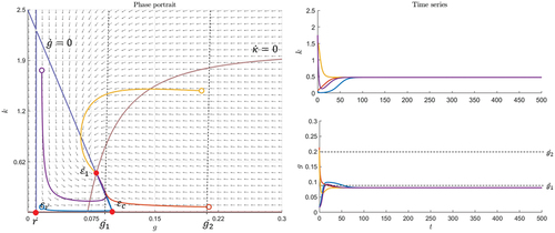
Figure 1. Euphoric scenario with stable and attractive spiral and parameters $r=0.01,\alpha =3,\beta =0.001,N=2,\mu =0.1,\lambda =0,c=0.$.

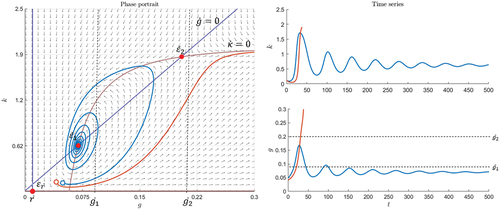
In Figure 1 there is an example of a situation with three equilibria and $\mu \in (0,1)$. The equilibrium ${\epsilon }_{\bar{r}}$ is a saddle, ${\tilde{\epsilon }}_1$ is a stable and attractive spiral, and ${\tilde{\epsilon }}_2$ is another saddle. Thus, all the trajectories that start in the region of attraction around ${\tilde{\epsilon }}_1$ will spiral toward this equilibrium (see blue trajectory in Figure 1). In this case, the market stabilizes itself each time an exogenous shock leads to a scenario inside the region of attraction of ${\tilde{\epsilon }}_1$. However, if there is a shock that brings the system to a scenario outside this region, it can be seen in Figure 1 that the trajectory converges to the case where $\kappa$ approaches the carrying capacity, ${lim}_{t\to \mathrm{\infty }}\kappa (t)=N$, and $g$ continues to grow (see orange trajectory in Figure 1). A bubble emerges when $g$ rises above the threshold $\bar{g}$. In the latter case (see orange trajectory in Figure 1), $g$ continues growing and therefore exceeds any choice of $\bar{g}$ at some time. The bubble bursts at time $\tau$. Whether a bubble emerges when the market shows the spiral behavior depends on the bubble threshold. If $\bar{g}$ is small enough, for example, ${\bar{g}}_1$, so that the spiral trajectory crosses this threshold, the bubble deflates and the market is corrected within the cycle (see blue trajectory in Figure 1). In this case, a sufficient number of individuals believe in overpricing, so that the trajectory crosses the $\dot{g}=0$ isocline and $g$ starts to decrease. In the next cycle, the bubble rises and deflates again, but in each further cycle the variables have smaller dynamics until the trajectory no longer reaches sufficiently high values for $g$. The bubble is corrected endogenously. If $g$ is high, for example, ${\bar{g}}_2$, bubbles can only emerge when an exogenous shock leads to a trajectory outside the region of attraction of ${\tilde{\epsilon }}_1$.

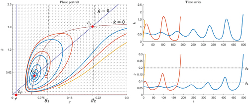
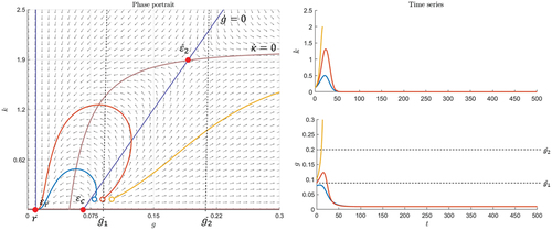
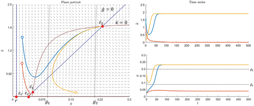
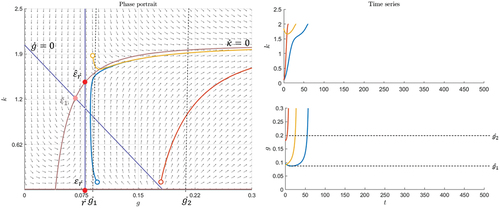
Figure 2 shows an example, in which the equilibrium ${\tilde{\epsilon }}_1$ is an unstable spiral and $\mu \in (0,1)$ again. The other equilibria ${\epsilon }_{\bar{r}}$ and ${\tilde{\epsilon }}_2$ are saddles again. In this case, each trajectory eventually moves toward the bubble scenario—either cyclically or directly. If it starts close to the equilibrium ${\tilde{\epsilon }}_1$ and $\bar{g}$ is sufficiently small, for example, ${\bar{g}}_1$, a bubble emerges in every cycle and an even larger bubble arises in the next cycle (see blue trajectory and the lower time series in Figure 2). During this cyclic phase, the bubbles deflate and the next bubble starts until one eventually remains. This bubble bursts at time $\tau$. If an exogenous shock brings the system to a point with some distance to ${\tilde{\epsilon }}_1$, for instance, if $g$ is high (see yellow trajectory in Figure 2), the bubble scenario is reached without cyclic movement. In this case, the bubble also bursts at $\tau$. Compared to the example in Figure 1, only the parameters for the flow of information are different in Figure 2. Thus, I conclude that the way in which the information that makes individuals believe in overpricing is spread and the rate at which people stop believing influences stability and therefore long-term market behavior.

Figure 2. Euphoric scenario with unstable spiral and parameters$r=0.01,\alpha =2,\beta =0.005,N=2,\mu =0.1,\lambda =0.1,c=0$.

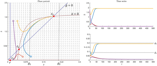
In Figure 3 there is a different and very interesting scenario in which the parameters are only slightly different from the previous examples. The fixed points ${\epsilon }_{\bar{r}}$ and ${\tilde{\epsilon }}_2$ are saddles and ${\tilde{\epsilon }}_1$ is another unstable spiral. However, in the long-run, a limit cycle arises. All neighboring trajectories approach the limit cycle as time approaches infinity. Thus, this limit cycle is stable. Its shape provides more insights into market behavior. Suppose the system starts in the bottom left-hand corner where $\kappa$ is at its cycle minimum and $\dot{\kappa }=0$, which means that there is no change in beliefs about overpricing and very few investors believe that prices are abnormally high. The growth rate $g$ is also small at this point. However, $\dot{g}>0$, which implies that the growth rate increases first. This causes movement to the right, where $\kappa$ then also increases. So, the system moves on an anti-clockwise direction. More people believe in overpricing. Therefore, the system moves to a point where the growth in $g$ slows down until it is at its cycle maximum, $\dot{g}=0$. This means there is no change in growth, but still $\dot{\kappa }>0$ and, thus, it moves upward toward the area where $\dot{g}<0$. Here, the growth rate decreases. Thus, the system gets to the point where $\dot{\kappa }=0$ again and $\kappa$ is maximal, but still $\dot{g}<0$, which causes movement to the left where $\kappa$ is also decreasing. So, a decreasing growth rate causes more investors to change their mind and stop believing in overpricing. Thus, both variables decline until the point where $\dot{g}=0$ is reached again. At this point, $g$ has its minimum value in the cycle, but $\kappa$ is still decreasing. There are thus still investors who stop perceiving overpricing while the growth rate is very small. Finally, the system returns to its starting point and the next cycle begins.

Figure 3. Euphoric scenario with unstable spiral yielding a limit cycle and parameters $r=0.01,\alpha =3,\beta =0.005,N=2,\mu =0.1,\lambda =0.11,c=0$.

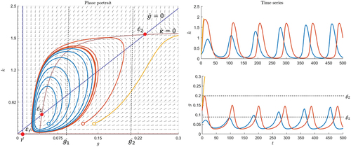
Based on the assumption for $\tau$, it is not possible for a bubble to bursts where the trajectory approaches the limit cycle. Rather, prices are observed being corrected and any possible bubbles, for example, if the threshold is ${\bar{g}}_1$, deflate and the next bubble starts growing. In this example, bubbles emerge in every cycle. If the bubble threshold is high, for instance, ${\bar{g}}_2$, a bubble only emerges in trajectories outside the region of attraction of the limit cycle and bursts at time $\tau$.

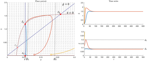
Figure 4 and Figure 5 provide examples for $\mu >1$. In this case, the slope of the isocline $\dot{g}=0$ is negative and the equilibrium ${\epsilon }_c$ exists. In both examples, it is a saddle and ${\epsilon }_{\bar{r}}$ is another saddle. However, the equilibrium ${\tilde{\epsilon }}_1$ causes different market behavior. In Figure 4, ${\tilde{\epsilon }}_1$ is a stable and attractive spiral. Taking a look at the time series on the right in Figure 4, it can be seen that all the trajectories move toward ${\tilde{\epsilon }}_1$ very fast. Bubbles can only emerge when $\bar{g}$ is sufficiently small, for instance, ${\bar{g}}_1$. Based on the assumption for $\tau$ these bubbles cannot burst. Each bubble deflates quickly and the system spirals toward the equilibrium ${\tilde{\epsilon }}_1$. In Figure 5, the fixed point ${\tilde{\epsilon }}_1$ is a stable and attractive node. Behavior is similar to the latter case, but in this example the system moves directly toward the fixed point ${\tilde{\epsilon }}_1$ and does not show cyclic movements. The bubble scenario can also only emerge for a short time and will be corrected without a bubble bursting.

Figure 4. Euphoric scenario with stable and attractive spiral and parameters$r=0.01,\alpha =3,\beta =0.007,N=2,\mu =2,\lambda =0.5,c=-0.5$.

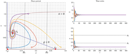
Figure 5. Euphoric scenario with stable and attractive node and parameters $r=0.01,\alpha =2,\beta =0.01,N=2,\mu =6,\lambda =0.2,c=-0.5$.

In Figure 6 there is an example with $\mu <0$, in which ${\epsilon }_{\bar{r}}$ is a stable and attractive node and ${\epsilon }_c$ is an unstable node. The fixed point ${\tilde{\epsilon }}_1$ is not located in the sensible-phase space $P$, and ${\tilde{\epsilon }}_2$ is a saddle. Those trajectories that start in the region of attraction of ${\epsilon }_{\bar{r}}$ move toward this equilibrium. This can happen in a semicircle. Considering the orange trajectory in Figure 6, it is seen that at first both $g$ and $\kappa$ increase until $g$ reaches its maximum and $\dot{g}=0$. Then, first $g$ decreases and later also $\kappa$ until ${\epsilon }_{\bar{r}}$ is reached. Thus, if the bubble threshold is low, for example, ${\bar{g}}_1$, a bubble can emerge and deflate. Outside the attraction region trajectories move toward the bubble scenario (see yellow trajectory in Figure 6) until the bubble bursts at $\tau$.

Figure 6. Euphoric scenario with stable and attractive node and parameters$r=0.01,\alpha =2,\beta =0.005,N=2,\mu =-0.5,\lambda =0.1,c=0.1$.

Thus, in the euphoric case, many different types of equilibria and long-term behaviors are found. If agents try to increase their returns by means of increased savings when more agents already believe in overpricing, the market can move in both stable and unstable cycles. If the savings rate is highly dependent on $g$ ($\mu >1$, see Figures 4 and 5), the system may always move toward a stable equilibrium. In this case, the bubbly scenario is left endogenously and any possible bubbles do not burst. When the savings rate is only weakly or even negatively dependent on $g$ ($\mu <1$, see Figures 1, Figures 2, 3, and Figure 6), exogenous shocks can take the system toward the bubbly scenario in which the bubble bursts.

3.2. The cautious scenario

If $\lambda <0$, investors decrease additional savings when more individuals believe in overpricing. This is called the cautious scenario, as this reflects the behavior of more risk-averse traders. In this scenario, no cyclic behavior is found. Instead, there are more stable and attractive-fixed points. For example, the equilibrium $(\bar{r},0)$ can be stable and attractive. If there are two equilibria ${\tilde{\epsilon }}_1$ and ${\tilde{\epsilon }}_2$, then ${\tilde{\epsilon }}_2$ can be stable and attractive as well. Thus, in this scenario the system moves directly toward one of these equilibria if it starts in their region of attraction. Consequently, the growth rate $g$ does not continue growing, which makes the occurrence of a bubble more unlikely than in the euphoric scenario, and if bubbles do emerge, they are more likely corrected. Furthermore, bubbles cannot emerge and deflate several times endogenously. These findings are summarized in the following Theorem:

Theorem 3.2.

In the cautious scenario ($\lambda <0$), there exist the following types of equilibria:

1. If $\mu <1$, the equilibrium ${\tilde{\epsilon }}_1$ can be a saddle. When $\mu >1$, ${\tilde{\epsilon }}_1$ can be a saddle and ${\tilde{\epsilon }}_2$ can be a stable and attractive node.

2. The equilibrium ${\epsilon }_{\bar{r}}$ can be a stable and attractive node or a saddle.

3. If the equilibrium ${\epsilon }_c$ exists, it can be an unstable node or a stable and attractive node.

Proof of this Theorem is provided in Appendix D. The same strategy as in the euphoric case described in the above is used. Thus, some examples are discussed, in which the market behaves as mentioned in Theorem 3.2.

In Figure 7 there is an example in which ${\epsilon }_{\bar{r}}$ and ${\tilde{\epsilon }}_2$ are stable and attractive nodes and $\mu >1$. Between these stable equilibria there is a saddle ${\tilde{\epsilon }}_1$. If the system starts close to ${\epsilon }_{\bar{r}}$, it will move toward this equilibrium. Otherwise, it moves toward ${\tilde{\epsilon }}_2$. In this case, the growth rate $g$ cannot continue growing until a bubble bursts. If the bubble threshold is high, for example, ${\bar{g}}_2$, a bubble can only exist for a while after an exogenous shock and then deflates. If it is low, for example, ${\bar{g}}_1$, a bubble can exist in the stable equilibrium $\bar{g}\le {\tilde{g}}_2$. In this model’s definition of $\tau$ this bubble never bursts because $g$ does not continue growing in equilibrium.

Figure 7. Cautious scenario with saddle and stable and attractive node and parameters$r=0.01,\alpha =3,\beta =0.005,N=2,\mu =2,\lambda =-0.1,c=0$.

In Figure 8 the equilibrium ${\epsilon }_{\bar{r}}$ is a stable node and ${\tilde{\epsilon }}_1$ is a saddle. There is $\mu <0$. Further, ${\epsilon }_c$ is an unstable node. In this case, the system either moves toward the stable equilibrium ${\epsilon }_{\bar{r}}$ or toward the bubble scenario where $g$ continues to grow until the bubble bursts at time $\tau$. Only if the bubble threshold is small enough, for example ${\bar{g}}_1$, so that it is within the attraction region of ${\epsilon }_{\bar{r}}$, can a bubble deflate.

Figure 8. Cautious scenario with saddle and parameters$r=0.01,\alpha =3,\beta =0.005,N=2,\mu =-0.1,\lambda =-0.1,c=0.2$.

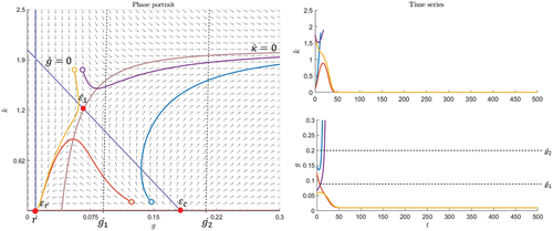
Figure 9 also shows an example with two stable and attractive nodes, ${\epsilon }_c$ and ${\tilde{\epsilon }}_2$. The dynamics are similar to the case in Figure 7, but here ${\epsilon }_c$ exists and is a stable node.

Figure 9. Cautious scenario with two stable nodes and parameters$r=0.01,\alpha =2,\beta =0.005,N=2,\mu =2,\lambda =-0.1,c=-0.04$.

Thus, in the cautious scenario not as many different outcomes as in the euphoric scenario are found. If agents show more risk-averse behavior and reduce their savings when more people believe in abnormally high asset prices, there always exist stable equilibria. If savings are weakly or negatively dependent on the growth rate $g$ ($\mu <1$), a stable fixed point is approached from any starting point. In such cases, bubbles can only persist for short periods of time and deflate endogenously. If savings are strongly dependent on $g$ ($\mu >1$), it is possible that a bubble will burst.

3.3. Impacts of monetary policy

As mentioned in the above, there is an ongoing debate about, whether central banks should only react to inflation in relation to goods prices or whether they should also react to inflation in relation to asset prices. Therefore, in this section, the effects of an interest rate increase are studied in the different financial market scenarios. This answers the third research question: Is there a difference in market behavior when a central bank intervenes by increasing the interest rate?

Figure 10 and Figure 11 illustrate the impact of an increase in the riskless return $\bar{r}$ in the euphoric scenario. Recall that only those trajectories that are located on the isocline $g=\bar{r}$ or are to its right are sensible in this model. Therefore, in this case, the equilibrium ${\hat{\epsilon }}_{\bar{r}}=\left(\bar{r},N-\frac{N\beta }{\alpha {\bar{r}}^2}\right)$ exists. In the example in Figure 10, this is a stable and attractive node. The remaining parameters in the example in Figure 10 are equal to those in the example in Figure 1. Recall that in Figure 1 the equilibrium ${\tilde{\epsilon }}_1$ is a stable spiral. In Figure 10 the right-hand semicircle starts as in Figure 1, but it stops and remains in ${\hat{\epsilon }}_{\bar{r}}$. Although the growth rate is equal to the riskless return, there are individuals who believe that prices are abnormally high at this fixed point. Thus, this stable equilibrium ${\hat{\epsilon }}_{\bar{r}}$ is approached directly and not after going through several cycles like ${\tilde{\epsilon }}_1$ in Figure 1. Further, both $g$ and $\kappa$ are greater at this fixed point after an increase in $\bar{r}$.

Figure 10. Euphoric scenario with higher return and parameters$r=0.08,\alpha =3,\beta =0.01,N=2,\mu =0.1,\lambda =0.1,c=0$.

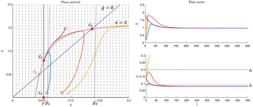
Figure 11. Cautious scenario with higher return and parameters$r=0.08,\alpha =3,\beta =0.01,N=2,\mu =-1,\lambda =-0.1,c=0.1$.

A very similar result is depicted in Figure 11. The parameters are equal to those in the example in Figure 3 in the euphoric scenario, in which a limit cycle exists. If $\bar{r}$ is increased so that $g$ approaches $\bar{r}$ within the cycle, the cyclic movement ends when the equilibrium ${\hat{\epsilon }}_{\bar{r}}$ is reached.

In Figures 12 and 13, both examples of the cautious scenario, a change in market behavior after increasing $\bar{r}$ is also observed. The remaining parameters in Figure 12 are equal to those in Figure 7. In Figure 12 the fixed point ${\epsilon }_{\bar{r}}$ is a saddle; in Figure 7 it is a stable node. Thus, after increasing $\bar{r}$ the system does not stay at this fixed point. Instead, it keeps moving toward the greater equilibrium ${\tilde{\epsilon }}_2$.

Figure 12. Euphoric scenario with higher return and parameters$r=0.08,\alpha =3,\beta =0.005,N=2,\mu =0.1,\lambda =0.11,c=0$.

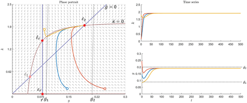
Figure 13. Cautious scenario with higher return and parameters$r=0.08,\alpha =3,\beta =0.005,N=2,\mu =-0.1,\lambda =-0.1,c=0.2$.

A very similar result is illustrated in Figure 13. The parameters are the same in Figure 8. In this case, the increase in $\bar{r}$ leads to a scenario without stable equilibria, although ${\epsilon }_{\bar{r}}$ is stable when $\bar{r}$ is low.

Proofs for these types of new equilibria can be found in Appendix E. It can be learned from these examples that the system can behave differently when the riskless return $\bar{r}$ is increased. This leads to the question of whether a central bank should intervene when there are bubbles. In the examples in Figures 10 and 11, it is possible to stop the bubble bursting as long as there is no exogenous shock that takes the system outside of the attraction region of the equilibrium ${\hat{\epsilon }}_{\bar{r}}$, but this behavior is similar to the case in which $\bar{r}$ is low and ${\tilde{\epsilon }}_1$ is stable. The difference here, though, is that bubbles cannot emerge and deflate several times endogenously when the bubble threshold is low, for example ${\bar{g}}_1$, because cyclic movement is prevented. Instead, the system moves more quickly toward the new stable-fixed point ${\hat{\epsilon }}_{\bar{r}}$. Thus, increasing the interest rate can stabilize the system more quickly. However, at the new stable-fixed point both $g$ and $\kappa$ are greater. This is also true of the example in Figure 12. In this case, only the large stable node remains after the increase in $\bar{r}$. If the bubble threshold is low, for example ${\bar{g}}_1$, a bubble can persist in equilibrium, which is also true when $\bar{r}$ is low. Further, with both values for $\bar{r}$, bubbles cannot burst in these examples. The impact that is shown in Figure 13 supports those who oppose central bank intervention. As the increase in $\bar{r}$ removes the stable equilibrium, all the trajectories move toward the bubble scenario and the bubble bursts at $\tau$.

Hence, in this financial market system, increasing the interest rate does not prevent bubbles and the possibility that they will burst. However, it may stabilize the system so that bubbles cannot emerge and deflate in cycles endogenously.

4. Summary and conclusion

In this paper, a two-dimensional system of differential equations is developed to describe long-term financial market behavior based on the ideas of Abreu and Brunnermeier (2003). In doing so, the following questions are answered: (1) What is the long-term market behavior under different behavioral phenomena? (2) When do bubbles emerge? Do bubbles always burst or can they deflate? (3) Is there a difference in market behavior when a central bank intervenes by increasing the interest rate?

To answer the first question, the long-term behavior is studied in a phase plane analysis by dividing the setting into two scenarios—the euphoric scenario and the cautious scenario—depending on an individual’s response to information about other traders’ beliefs. Very different outcomes are obtained, which are summarized in Table 1. This setup shows that the financial market system contains both stable and unstable equilibria. It is shown under which conditions these equilibria are spirals and even approach limit cycles. If agents are euphoric, which means that they try to increase their returns by means of increased savings while more investors believe in the existence of overpricing, the model incorporates cycles both exogenously and endogenously. Thus, for example, when traders show herding behavior or try to ride potential bubbles, financial markets show cyclic movements. This market behavior can even lead to a limit cycle. Differences in the processing of information yield different market behavior in the long term, for instance, if the cycles are stable or unstable. In the cautious scenario, there are no cycles like in the euphoric scenario. Instead, more stable equilibria are found. Thus, when investors are more cautious and reduce their savings, while more overpricing is perceived, financial markets reach stable equilibria.

Table 1. Summary of the different types of equilibria that are found in the two scenarios (see Theorem 3.1 and Theorem 3.2)

		euphoric scenario(λ>0)	cautious scenario(λ<0)
${\tilde{\epsilon }}_i$	$\mu <1$	stable and attractive spiral unstable spiral unstable spiral with limit cycle	saddle
	$\mu >1$	stable spiral stable and attractive node	stable and attractive node saddle
${\epsilon }_{\bar{r}}$	$\mu <0$	stable and attractive node saddle	stable and attractive node saddle
	$\mu >1$	saddle	stable and attractive nodesaddle
${\epsilon }_c$		unstable node saddle	stable and attractive node unstable node

The second question is answered by introducing an exogenous bubble threshold to the model. This indicates when asset prices exceed their fundamental value. The existence of bubbles depends on this bubble threshold. Bubbles can occur in both the euphoric and the cautious scenario. When cycles occur or stable equilibria exist, bubbles can emerge and deflate as the growth rate $g$ can be reduced endogenously. When the system is moved outside of the region of attraction of a stable equilibrium the bubble continues to grow until it eventually bursts. This latter case is found in both scenarios. However, in the euphoric scenario, when cycles occur and the bubble threshold is sufficiently low, bubbles emerge and deflate even more often.

To answer the third question, the impact of increasing the interest rate on long-term behavior is examined. The result is that monetary policy can be used as a direct means to stabilize the market and prevent cyclic movement, because new stable equilibria are approached. However, this does not prevent bubbles emerging and bursting. If the bubble threshold is low, the bubble scenario can still be reached and outside of the region of attraction of stable equilibria bubbles can still burst. Moreover, high asset price growth can be flattened and market volatility can be decreased. This reduces the investment risk.

Disclosure statement

No potential conflict of interest was reported by the author.

Data availability statement

Data sharing is not applicable to this article as no new data were created or analyzed in this study.

Additional information

Notes on contributors

Carina Burs

Carina Burs is a postdoctoral researcher at the Economics Department at Paderborn University, Germany. She holds both a bachelor’s degree and a master’s degree in Mathematics as well as a PhD in Economics. Her research interests include the theoretical work on the role of information in decision processes, ideologies and financial bubbles.

Notes

1. See Markowitz (1959), pp. 286–287.

2. In AB, this is a fraction.

3. See Murray (1989), for example.

4. AB model the price process with $p_t(g)=e^{gt}$, where from a random time on the fraction $(1-\beta )p_t$ represents the fundamental value and the fraction $\beta p_t$ is the bubble component.

Appendix A.

Utility Function

Textbooks often include this setting with absolute values of return $R$ and, therefore, wealth at the end of one period is $W_1=W_0+R$. However, in this paper, the Markowitz model is analyzed regarding the rates of return $r$ that we can easily rearrange to

$W_1=W_0+R_{abs}=W_0\left(1+\frac{W_0}{R_{abs}}\right)=W_0(1+r).$

$R_{abs}$ is an expected absolute return and $r$ is an expected rate of return. Expected utility is

$U=\mathbb{E}[u(W_1)]=\mathbb{E}[W_1-\frac{1}{2}A{W}_1^2]$

$=\mathbb{E}[W_1]-\frac{1}{2}A\mathbb{E}[W_1^2]=\mathbb{E}[W_1]-\frac{1}{2}AVar(W_1)-\frac{1}{2}A\mathbb{E}[W1{]}^2$

$=\mathbb{E}[W_0(1+r)]-\frac{1}{2}AVar(W_0(1+r))-\frac{1}{2}A\mathbb{E}[W_0(1+r){]}^2$

$=W_0(1+{\mu }_r)-\frac{1}{2}A{W}_0{\sigma }_r^2-\frac{1}{2}A(W_0(1+r){)}^2.$

As utility is invariant under transformation, only

$\tilde{U}=W_0(1+{\mu }_r)-\frac{1}{2}A{W}_0^2{\sigma }_r^2$

is considered for simplicity without loss of generality.

Appendix B.

The Markowitz Model

B.1. Capital Market Line

Investors can choose each combination of the risky market portfolio $m$ and a risk-free asset, which is called portfolio $p$. Then the rate of return of $p$ is

$R_p=\alpha R_m+(1-\alpha )\bar{r}=\bar{r}+\alpha (g-\bar{r})\mathrm{w}\mathrm{i}\mathrm{t}\mathrm{h}\alpha \in [0,1]$

and the expected return of $p$ is

$r_p=\alpha r_m+(1-\alpha )\bar{r}=\bar{r}+\alpha (r_m-\bar{r})\mathrm{w}\mathrm{i}\mathrm{t}\mathrm{h}\alpha \in [0,1].$

The variance of portfolio $p$ is

${\sigma }_p^2=Var(R_p)$

$=Var(\alpha R_m+(1-\alpha )\bar{r})$

$={\alpha }^2{\sigma }_m^2+2\alpha (1-\alpha )Cov(R_m,\bar{r})+(1-\alpha {)}^{2}Var(\bar{r})$

$={\alpha }^2{\sigma }_m^2$

because $Var(\bar{r})=0$ and $Cov(R_m,\bar{r})=E[(R_m-r_m)(\bar{r}-\bar{r})]=0$. The standard deviation of $p$ is

${\sigma }_p=\alpha {\sigma }_m.$

Hence, there is a linear relationship which can be summarized in the following line equation

$\left(\begin{array}{c}{\sigma }_p\\ r_p\end{array}\right)=\left(\begin{array}{c}0\\ \bar{r}\end{array}\right)+\alpha \left(\begin{array}{c}{\sigma }_m\\ r_m-\bar{r}\end{array}\right).$

Consequently,

$r_p=\bar{r}+(r_m-\bar{r})\frac{{\sigma }_p}{{\sigma }_m}$

which is the equation for the capital market line (CML). Thus, $\frac{(r_m-\bar{r})}{{\sigma }_m}$ is the slope of the CML. The difference $(r_m-\bar{r})$ is a measure of the risk premium and, therefore, the slope measures the reward per unit of market risk.

B.1.1. Utility Maximization

A portfolio’s rate of return is given by

$R_p={\theta }_m{R}_m+{\theta }_f\bar{r}$

and the expected return is

$r_p={\theta }_m{r}_m+{\theta }_f\bar{r}.$

As in B.1, the variance of the portfolio can be calculated as

$Var(R_p)={\sigma }_p^2={\theta }_m^{2}Var(R_m)+2{\theta }_m{\theta }_{f}Cov(R_m,\bar{r})+{\theta }_f^{2}Var(\bar{r})$

$={\theta }_m^{2}Var(R_m)$

$={\theta }_m^2{\sigma }_m^2.$

Using this, utility can be rewritten obtaining

$U=\mathbb{E}[W_1]-\frac{1}{2}AVar(W_1)$

$=\mathbb{E}[W_0(1+R_p)]-\frac{1}{2}AVar(W_0(1+R_p))$

$=W_0(1+r_p)-\frac{1}{2}A{W}_0^{2}Var(R_p)$

$=W_0(1+{\theta }_m{r}_m+{\theta }_f\bar{r})-\frac{1}{2}A{W}_0^2{\theta }_m^2{\sigma }_m^2.$

Hence, the optimization problem of maximizing utility is

$max{W}_0+W_0{\theta }_m{r}_m+W_0{\theta }_f\bar{r}-\frac{1}{2}A{W}_0^2{\theta }_m^2{\sigma }_m^2$

$\mathrm{s}.\mathrm{t}.{\theta }_f+{\theta }_m=1.$

This can be solved using the Lagrangian method. When $\lambda$ is the Lagrange multiplier, the following equations are obtained:

$W_0{r}_m-A{W}_0^2{\theta }_m{\sigma }_m^2+\lambda =0$

$W_0\bar{r}+\lambda =0$

${\theta }_f+{\theta }_m=1.$

From the second equation it follows

$\lambda =-W_0\bar{r}.$

Plugging this into the first equation it is

${\theta }_m=\frac{r_m-\bar{r}}{A{W}_0{\sigma }_m^2}$

and using this in the third equation the result is

${\theta }_f=1-\frac{r_m-\bar{r}}{A{W}_0{\sigma }_m^2}.$

The bordered Hessian can be used to make sure that the result maximizes utility. This is

$\bar{H}=\left(\begin{array}{ccc}0& 1& 1\\ 1& -A{W}_0^2{\sigma }_m^2& 0\\ 1& 0& 0\end{array}\right).$

Thus,

$det(\bar{H})=A{W}_0^2{\sigma }_m^2>0,$

which implies that a maximum is found.

Appendix C.

Proof of Theorem 3.1

It is shown that certain choices of parameters yield the desired types of equilibria.

(a) o Choose the parameters $r=0.01,\alpha =3,\beta =0.01,N=2,\mu =0.1,\lambda =0.1,c=0$ (see Figure 1). Then, the Jacobian in equilibrium ${\tilde{\epsilon }}_1=(0.07,0.63)$ is

$J({\tilde{\epsilon }}_1)=\left(\begin{array}{cc}0.054& -0.006\\ 2.58& -0.066\end{array}\right)$

with eigenvalues ${\lambda }_1=0.01$ and ${\lambda }_2=-0.97$. Further, $det(J({\tilde{\epsilon }}_1))=0.0119$ and $\mathrm{t}\mathrm{r}(J({\tilde{\epsilon }}_1))=-0.0120$.

Thus, $\mathrm{t}\mathrm{r}(J({\tilde{\epsilon }}_1){)}^2<4det(J({\tilde{\epsilon }}_1))$ and $\mathrm{t}\mathrm{r}(J({\tilde{\epsilon }}_1))<0$, which implies that the equilibrium ${\tilde{\epsilon }}_1$ is a stable spiral.

o Choose the parameters $r=0.01,\alpha =2,\beta =0.005,N=2,\mu =0.1,\lambda =0.1,c=0$ (see Figure 2). Then, the Jacobian in equilibrium ${\tilde{\epsilon }}_1=(0.06,0.52)$ is

$J({\tilde{\epsilon }}_1)=\left(\begin{array}{cc}0.043& -0.005\\ 1.55& -0.03\end{array}\right)$

with eigenvalues ${\lambda }_1=0.01-0.08i$ and ${\lambda }_2=0.01+0.08i$. Further, $det(J({\tilde{\epsilon }}_1))=0.0065$ and $\mathrm{t}\mathrm{r}(J({\tilde{\epsilon }}_1))=0.0130$.

Thus, $\mathrm{t}\mathrm{r}(J({\tilde{\epsilon }}_1){)}^2<4det(J({\tilde{\epsilon }}_1))$ and $\mathrm{t}\mathrm{r}(J({\tilde{\epsilon }}_1))>0$, which implies that the equilibrium ${\tilde{\epsilon }}_1$ is an unstable spiral.

o Choose the parameters $r=0.01,\alpha =3,\beta =0.005,N=2,\mu =0.1,\lambda =0.11,c=0$. (see Figure 3). Then, the Jacobian in equilibrium ${\tilde{\epsilon }}_1=(0.04,0.37)$ is

$J({\tilde{\epsilon }}_1)=\left(\begin{array}{cc}0.032& -0.004\\ 1.81& -0.025\end{array}\right)$

with eigenvalues ${\lambda }_1=0-0.08i$ and ${\lambda }_2=0+0.08i$. Further, $det(J({\tilde{\epsilon }}_1))=0.0064$ and $\mathrm{t}\mathrm{r}(J({\tilde{\epsilon }}_1))=0.0070$.

Thus, $\mathrm{t}\mathrm{r}(J({\tilde{\epsilon }}_1){)}^2<4det(J({\tilde{\epsilon }}_1))$ and $\mathrm{t}\mathrm{r}(J({\tilde{\epsilon }}_1))>0$, which implies that the equilibrium ${\tilde{\epsilon }}_1$ is an unstable spiral. Additionally, it can be seen in Figure 3 that there is a finite region $R$ in the plane that lies between two simple closed curves. At each point on these curves, the vector field points toward the interior of the region $R$ and $R$ does not contain any critical points. Thus, the existence of a limit cycle follows from the Poincaré-Bendixson Theorem.

o Choose the parameters $r=0.01,\alpha =3,\beta =0.007,N=2,\mu =2,\lambda =0.5,c=-0.5$ (see Figure 4). Then, the Jacobian in equilibrium ${\tilde{\epsilon }}_1=(0.06,0.87)$ is

$J({\tilde{\epsilon }}_1)=\left(\begin{array}{cc}-0.054& -0.027\\ 2.95& -0.084\end{array}\right)$

with eigenvalues ${\lambda }_1=-0.07-0.28i$ and ${\lambda }_2=-0.07+0.08i$. Further, $det(J({\tilde{\epsilon }}_1))=0.0842$ and $\mathrm{t}\mathrm{r}(J({\tilde{\epsilon }}_1))=-0.138$.

Thus, $\mathrm{t}\mathrm{r}(J({\tilde{\epsilon }}_1){)}^2<4det(J({\tilde{\epsilon }}_1))$ and $\mathrm{t}\mathrm{r}(J({\tilde{\epsilon }}_1))<0$, which implies that the equilibrium ${\tilde{\epsilon }}_1$ is a stable spiral.

o Choose the parameters $r=0.01,\alpha =2,\beta =0.01,N=2,\mu =6,\lambda =0.2,c=-0.5$ (see Figure 5). Then, the Jacobian in equilibrium ${\tilde{\epsilon }}_1=(0.08,0.47)$ is

$J({\tilde{\epsilon }}_1)=\left(\begin{array}{cc}-0.355& -0.01\\ 1.45& -0.038\end{array}\right)$

with eigenvalues ${\lambda }_1=-0.26$ and ${\lambda }_2=-0.13$. Further, $det(J({\tilde{\epsilon }}_1))=0.0338$ and $\mathrm{t}\mathrm{r}(J({\tilde{\epsilon }}_1))=-0.393$.

Thus, $\mathrm{t}\mathrm{r}(J({\tilde{\epsilon }}_1){)}^2>4det(J({\tilde{\epsilon }}_1))$, $det(J({\tilde{\epsilon }}_1))>0$, and $\mathrm{t}\mathrm{r}(J({\tilde{\epsilon }}_1))<0$, which implies that the equilibrium ${\tilde{\epsilon }}_1$ is a stable node.

(b) o Choose the parameters $r=0.01,\alpha =3,\beta =0.01,N=2,\mu =0.1,\lambda =0.1,c=0$ (see Figure 1). Then, the Jacobian in equilibrium ${\epsilon }_{\bar{r}}=(0.01,0)$ is

$J({\epsilon }_{\bar{r}})=\left(\begin{array}{cc}0.009& 0\\ 0& -0.97\end{array}\right)$

with eigenvalues ${\lambda }_1=0.01$ and ${\lambda }_2=-0.97$. Further, $det(J({\epsilon }_{\bar{r}}))=-0.00873$ and $\mathrm{t}\mathrm{r}(J({\epsilon }_{\bar{r}}))=-0.961$.

Thus, $det(J({\epsilon }_{\bar{r}}))<0$ and $\mathrm{t}\mathrm{r}({\epsilon }_{\bar{r}}))\ne 0$, which implies that the equilibrium ${\epsilon }_{\bar{r}}$ is a saddle.

o Choose the parameters $r=0.01,\alpha =2,\beta =0.005,N=2,\mu =-0.5,\lambda =0.1,c=0.1$. (see Figure 6). Then, the Jacobian in equilibrium ${\epsilon }_{\bar{r}}=(0.01,0)$ is

$J({\epsilon }_{\bar{r}})=\left(\begin{array}{cc}-0.085& 0\\ 0& -0.48\end{array}\right)$

with eigenvalues ${\lambda }_1=-0.08$ and ${\lambda }_2=-0.48$. Further, $det(J({\epsilon }_{\bar{r}}))=0.0408$ and $\mathrm{t}\mathrm{r}(J({\epsilon }_{\bar{r}}))=-0.565$.

Thus, $\mathrm{t}\mathrm{r}(J({\epsilon }_{\bar{r}}){)}^2>4det(J({\epsilon }_{\bar{r}}))$, $det(J({\epsilon }_{\bar{r}}))>0$, and $\mathrm{t}\mathrm{r}(J({\epsilon }_{\bar{r}}))<0$, which implies that the equilibrium ${\epsilon }_{\bar{r}}$ is a stable node.

(c) o Choose the parameters $r=0.01,\alpha =2,\beta =0.005,N=2,\mu =-0.5,\lambda =0.1,c=0.1$. (see Figure 6). Then, the Jacobian in equilibrium ${\epsilon }_c=(0.07,0)$ is

$J({\epsilon }_c)=\left(\begin{array}{cc}0.085& -0.006\\ 0& 0.058\end{array}\right)$

with eigenvalues ${\lambda }_1=0.09$ and ${\lambda }_2=0.06$. Further, $det(J({\epsilon }_c))=0.00493$ and $\mathrm{t}\mathrm{r}(J({\epsilon }_c))=0.143$.

Thus, $\mathrm{t}\mathrm{r}(J({\epsilon }_c){)}^2>4det(J({\epsilon }_c))$, $det(J({\epsilon }_c))>0$, and $\mathrm{t}\mathrm{r}({\epsilon }_c))>0$, which implies that the equilibrium ${\epsilon }_c$ is an unstable node.

o Choose the parameters $r=0.01,\alpha =3,\beta =0.007,N=2,\mu =2,\lambda =0.5,c=-0.5$ (see Figure 4). Then, the Jacobian in equilibrium ${\epsilon }_c=(0.5,0)$ is

$J({\epsilon }_c)=\left(\begin{array}{cc}-0.49& -0.245\\ 0& 1.49\end{array}\right)$

with eigenvalues ${\lambda }_1=-0.49$ and ${\lambda }_2=1.49$. Further, $det(J({\epsilon }_c))=-0.7301$ and $\mathrm{t}\mathrm{r}(J({\epsilon }_c))=1$.

Thus, $det(J({\epsilon }_c))<0$ and $\mathrm{t}\mathrm{r}({\epsilon }_c))\ne 0$, which implies that the equilibrium ${\epsilon }_c$ is a saddle.

Appendix D.

Proof of Theorem 3.2

(a) o Choose the parameters $r=0.01,\alpha =3,\beta =0.005,N=2,\mu =2,\lambda =-0.1,c=0$. (see Figure 7). Then, the Jacobian in equilibrium ${\tilde{\epsilon }}_1=(0.05,0.47)$ is

$J({\tilde{\epsilon }}_1)=\left(\begin{array}{cc}-0.037& 0.004\\ 2.15& -0.033\end{array}\right)$

with eigenvalues ${\lambda }_1=-0.12$ and ${\lambda }_2=0.05$. Further, $det(J({\tilde{\epsilon }}_1))=-0.0074$ and $\mathrm{t}\mathrm{r}(J({\tilde{\epsilon }}_1))=-0.07$.

Thus, $det(J({\tilde{\epsilon }}_1))<0$ and $\mathrm{t}\mathrm{r}({\tilde{\epsilon }}_1))\ne 0$, which implies that the equilibrium ${\tilde{\epsilon }}_1$ is a saddle.

o Choose the parameters $r=0.01,\alpha =3,\beta =0.005,N=2,\mu =-0.1,\lambda =-0.1,c=0.2$. (see Figure 8). Then, the Jacobian in equilibrium ${\tilde{\epsilon }}_1=(0.07,1.26)$ is

$J({\tilde{\epsilon }}_1)=\left(\begin{array}{cc}0.063& 0.006\\ 2.79& -0.127\end{array}\right)$

with eigenvalues ${\lambda }_1=0.13$ and ${\lambda }_2=-0.19$. Further, $det(J({\tilde{\epsilon }}_1))=-0.0247$ and $\mathrm{t}\mathrm{r}(J({\tilde{\epsilon }}_1))=-0.064$.

Thus, $det(J({\tilde{\epsilon }}_1))<0$ and $\mathrm{t}\mathrm{r}({\tilde{\epsilon }}_1))\ne 0$, which implies that the equilibrium ${\tilde{\epsilon }}_1$ is a saddle.

o Choose the parameters $r=0.01,\alpha =3,\beta =0.005,N=2,\mu =2,\lambda =-0.1,c=0$. (see Figure 7). Then, the Jacobian in equilibrium ${\tilde{\epsilon }}_2=(0.19,1.91)$ is

$J({\tilde{\epsilon }}_2)=\left(\begin{array}{cc}-0.181& 0.018\\ 0.524& -0.546\end{array}\right)$

with eigenvalues ${\lambda }_1=-0.16$ and ${\lambda }_2=-0.57$. Further, $det(J({\tilde{\epsilon }}_2))=0.0894$ and $\mathrm{t}\mathrm{r}(J({\tilde{\epsilon }}_2))=-0.727$.

Thus, $\mathrm{t}\mathrm{r}(J({\tilde{\epsilon }}_2){)}^2>4det(J({\tilde{\epsilon }}_2))$, $det(J({\tilde{\epsilon }}_2))>0$, and $\mathrm{t}\mathrm{r}({\tilde{\epsilon }}_2))<0$, which implies that the equilibrium ${\tilde{\epsilon }}_2$ is a stable node.

(b) o Choose the parameters $r=0.01,\alpha =3,\beta =0.005,N=2,\mu =-0.1,\lambda =-0.1,c=0.2$. (see Figure 8). Then, the Jacobian in equilibrium ${\epsilon }_{\bar{r}}=(0.01,0)$ is

$J({\epsilon }_{\bar{r}})=\left(\begin{array}{cc}-0.189& 0\\ 0& -0.47\end{array}\right)$

with eigenvalues ${\lambda }_1=-0.19$ and ${\lambda }_2=-0.47$. Further, $det(J({\epsilon }_{\bar{r}}))=0.0888$ and $\mathrm{t}\mathrm{r}(J({\epsilon }_{\bar{r}}))=-0.659$.

Thus, $\mathrm{t}\mathrm{r}(J({\epsilon }_{\bar{r}}){)}^2>4det(J({\epsilon }_{\bar{r}}))$, $det(J({\epsilon }_{\bar{r}}))>0$ and $\mathrm{t}\mathrm{r}({\epsilon }_{\bar{r}}))<0$, which implies that the equilibrium ${\epsilon }_{\bar{r}}$ is a stable node.

o Choose the parameters $r=0.01,\alpha =2,\beta =0.005,N=2,\mu =2,\lambda =-0.1,c=-0.04$. (see Figure 9). Then, the Jacobian in equilibrium ${\epsilon }_{\bar{r}}=(0.01,0)$ is

$J({\epsilon }_{\bar{r}})=\left(\begin{array}{cc}0.03& 0\\ 0& -0.48\end{array}\right)$

with eigenvalues ${\lambda }_1=0.03$ and ${\lambda }_2=-0.48$. Further, $det(J({\tilde{\epsilon }}_1))=-0.0144$ and $\mathrm{t}\mathrm{r}(J({\tilde{\epsilon }}_1))=-0.45$.

Thus, $det(J({\epsilon }_{\bar{r}})<0$ and $\mathrm{t}\mathrm{r}({\epsilon }_{\bar{r}}))\ne 0$, which implies that the equilibrium ${\epsilon }_{\bar{r}}$ is a saddle.

(c) o Choose the parameters $r=0.01,\alpha =3,\beta =0.005,N=2,\mu =-0.1,\lambda =-0.1,c=0.2$. (see Figure 8). Then, the Jacobian in equilibrium ${\epsilon }_c=(0.18,0)$ is

$J({\epsilon }_c)=\left(\begin{array}{cc}0.189& 0.017\\ 0& 0.518\end{array}\right)$

with eigenvalues ${\lambda }_1=0.19$ and ${\lambda }_2=0.52$. Further, $det(J({\epsilon }_c))=0.0979$ and $\mathrm{t}\mathrm{r}(J({\epsilon }_c))=0.707$.

Thus, $\mathrm{t}\mathrm{r}(J({\epsilon }_c){)}^2>4det(J({\epsilon }_c))$, $det(J({\epsilon }_c))>0$, and $\mathrm{t}\mathrm{r}({\epsilon }_c))>0$, which implies that the equilibrium ${\epsilon }_c$ is an unstable node.

o Choose the parameters $r=0.01,\alpha =2,\beta =0.005,N=2,\mu =2,\lambda =-0.1,c=-0.04$. (see Figure 9). Then, the Jacobian in equilibrium ${\epsilon }_c=(0.04,0)$ is

$J({\epsilon }_c)=\left(\begin{array}{cc}-0.03& 0.003\\ 0& -0.045\end{array}\right)$

with eigenvalues ${\lambda }_1=-0.03$ and ${\lambda }_2=-0.05$. Further, $det(J({\epsilon }_c))=0.00135$ and $\mathrm{t}\mathrm{r}(J({\epsilon }_c))=-0.075$.

Thus, $\mathrm{t}\mathrm{r}(J({\epsilon }_c){)}^2>4det(J({\epsilon }_c))$, $det(J({\epsilon }_c))>0$, and $\mathrm{t}\mathrm{r}({\epsilon }_c))<0$, which implies that the equilibrium ${\epsilon }_c$ is a stable node.

Appendix E.

Proof of the Effects of Monetary Policy

- Choose the parameters $r=0.08,\alpha =3,\beta =0.01,N=2,\mu =0.1,\lambda =0.1,c=0$. (see Figure 10). Then, the Jacobian in equilibrium ${\hat{\epsilon }}_{\bar{r}}=(0.08,0.96)$ is

$J({\hat{\epsilon }}_{\bar{r}})=\left(\begin{array}{cc}-0.024& 0\\ 0& -0.115\end{array}\right)$

with eigenvalues ${\lambda }_1=-0.02$ and ${\lambda }_2=-0.12$. Further, $det(J({\hat{\epsilon }}_{\bar{r}}))=0.00276$ and $\mathrm{t}\mathrm{r}(J({\hat{\epsilon }}_{\bar{r}}))=-0.139$.

Thus, $\mathrm{t}\mathrm{r}(J({\hat{\epsilon }}_{\bar{r}}){)}^2>4det(J({\hat{\epsilon }}_{\bar{r}}))$, $det(J({\hat{\epsilon }}_{\bar{r}}))>0$, and $\mathrm{t}\mathrm{r}({\hat{\epsilon }}_{\bar{r}}))<0$, which implies that the equilibrium ${\hat{\epsilon }}_{\bar{r}}$ is a stable node.

- Choose the parameters $r=0.08,\alpha =3,\beta =0.005,N=2,\mu =0.1,\lambda =0.11,c=0$. (see Figure 11). Then, the Jacobian in equilibrium ${\hat{\epsilon }}_{\bar{r}}=(0.08,1.48)$ is

$J({\hat{\epsilon }}_{\bar{r}})=\left(\begin{array}{cc}-0.091& 0\\ 2.31& -0.178\end{array}\right)$

with eigenvalues ${\lambda }_1=-0.18$ and ${\lambda }_2=-0.09$. Further, $det(J({\hat{\epsilon }}_{\bar{r}}))=0.0162$ and $\mathrm{t}\mathrm{r}(J({\hat{\epsilon }}_{\bar{r}}))=-0.269$.

Thus, $\mathrm{t}\mathrm{r}(J({\hat{\epsilon }}_{\bar{r}}){)}^2>4det(J({\hat{\epsilon }}_{\bar{r}}))$, $det(J({\hat{\epsilon }}_{\bar{r}}))>0$, and $\mathrm{t}\mathrm{r}({\hat{\epsilon }}_{\bar{r}}))<0$, which implies that the equilibrium ${\hat{\epsilon }}_{\bar{r}}$ is a stable node.

- Choose the parameters $r=0.01,\alpha =3,\beta =0.01,N=2,\mu =-1,\lambda =-0.1,c=0.1$. (see Figure 12). Then, the Jacobian in equilibrium ${\epsilon }_{\bar{r}}=(0.08,0)$ is

$J({\epsilon }_{\bar{r}})=\left(\begin{array}{cc}-0.08& 0\\ 0& 0.177\end{array}\right)$

with eigenvalues ${\lambda }_1=0.18$ and ${\lambda }_2=-0.08$. Further, $det(J({\epsilon }_{\bar{r}})=-0.01416$ and $\mathrm{t}\mathrm{r}(J({\epsilon }_{\bar{r}}))=-0.0623$.

Thus, $det(J({\epsilon }_{\bar{r}})<0$ and $\mathrm{t}\mathrm{r}({\epsilon }_{\bar{r}}))\ne 0$, which implies that the equilibrium ${\epsilon }_{\bar{r}}$ is a saddle.

- Choose the parameters $r=0.01,\alpha =3,\beta =0.005,N=2,\mu =-0.1,\lambda =-0.1,c=0.2$. (see Figure 13). Then, the Jacobian in equilibrium ${\hat{\epsilon }}_{\bar{r}}=(0.08,1.48)$ is

$J({\hat{\epsilon }}_{\bar{r}})=\left(\begin{array}{cc}0.036& 0\\ 2.31& -0.178\end{array}\right)$

with eigenvalues ${\lambda }_1=-0.18$ and ${\lambda }_2=0.04$. Further, $det(J({\hat{\epsilon }}_{\bar{r}}))=-0.0064$ and $\mathrm{t}\mathrm{r}(J({\hat{\epsilon }}_{\bar{r}}))=-0.142$.

Thus, $det(J({\hat{\epsilon }}_{\bar{r}})<0$ and $\mathrm{t}\mathrm{r}({\hat{\epsilon }}_{\bar{r}}))\ne 0$, which implies that the equilibrium ${\hat{\epsilon }}_{\bar{r}}$ is a saddle.

References

- Abreu, D., & Brunnermeier, M. K. (2003). Bubbles and crashes. Econometrica, 71(1), 173–29. https://doi.org/10.1111/1468-0262.00393
- Ashiya, M., & Doi, T. (2001). Herd behavior of Japanese economists. Journal of Economic Behavior and Organization, 46(3), 343–346. https://doi.org/10.1016/s0167-2681(01)00182-2
- Bernanke, B. S., & Gertler, M. (1999). Monetary policy and asset price volatility. Economic Review, 84(Q IV), 17–51.
- Bikhchandani, S., Hirshleifer, D., & Welch, I. (1992). A theory of fads, fashion, custom, and cultural change as informational cascades. Journal of Political Economy, 100(5), 992–1026. https://doi.org/10.1086/261849
- Blanchard, O. J., & Watson, M. W. (1982). Bubbles, rational expectations and financial markets. NBER Working Paper Series, Working Paper No. w0945. https://doi.org/10.3386/w0945
- Bordo, M. D., Dueker, M. J., & Wheelock, D. C. (2002). Aggregate price shocks and financial instability: A historical analysis. Economic Inquiry, 40(4), 521–538. https://doi.org/10.1093/ei/40.4.521
- Brunnermeier, M. K. (2008). Bubbles. In Durlauf, S. N., & Blume, L. E.(Eds.), The new Palgrave dictionary of economics (pp. 1–8). Palgrave Macmillan UK.
- Brunnermeier, M. K., & Nagel, S. (2004). Hedge funds and the technology bubble. The Journal of Finance, 59(5), 2013–2040. https://doi.org/10.1111/j.1540-6261.2004.00690.x
- Cecchetti, S., Genberg, H., Lipsky, J., & Wadhwani, S. (2000). Geneva 2: Asset Prices and Central Bank Policy. CEPR Press.
- Daniel, K., Hirshleifer, D., & Subrahmanyam, A. (1998). Investor psychology and security market under- and overreactions. The Journal of Finance, 53(6), 1839–1885. https://doi.org/10.1111/0022-1082.00077
- De Bondt, W. F. M., & Thaler, R. (1985). Does the stock market overreact? The Journal of Finance, 40(3), 793–805. https://doi.org/10.1111/j.1540-6261.1985.tb05004.x
- Felipe, B., & Taylor, A. M. (2020). After the panic: Are financial crises demand or supply shocks? Evidence from International trade. American Economic Review: Insights, 2(4), 509–526. https://doi.org/10.1257/aeri.20190533
- Fritz, M., Gries, T., & Wiechers, L. 2022. An early indicator for anomalous stock market performance. Working papers CIE 153. Paderborn University, CIE Center for International Economics.
- Froot, K. A., & Obstfeld, M. (1991). Intrinsic bubbles: The case of stock prices. The American Economic Review, 81(5), 1189–1214.
- Galati, G., Hindrayanto, I., Jan Koopman, S., & Vlekke, M. (2016). Measuring financial cycles in a model-based analysis: Empirical evidence for the United States and the euro area. Economics Letters, 145, 83–87. https://doi.org/10.1016/j.econlet.2016.05.034
- Graham, J. R. (1999). Herding among investment newsletters: Theory and evidence. The Journal of Finance, 54(1), 237–268. https://doi.org/10.1111/0022-1082.00103
- Harrison, J. M., & David, M. K. (1978). Speculative investor behavior in a stock market with heterogeneous expectations. The Quarterly Journal of Economics, 92(2), 323. https://doi.org/10.2307/1884166
- Hördahl, P., & Packer, F. (2006). Understanding asset prices: An overview. BIS Papers, 34. https://doi.org/10.2139/ssrn.1190962
- Jegadeesh, N., & Titman, S. (1993). Returns to buying winners and selling losers: Implications for stock market efficiency. The Journal of Finance, 48(1), 65–91. https://doi.org/10.1111/j.1540-6261.1993.tb04702.x
- Jordà, Ò., Schularick, M., & Taylor, A. M. (2013). When credit bites back. Journal of Money, Credit and Banking, 45(s2), 3–28. https://doi.org/10.1111/jmcb.12069
- Kedar-Levy, H. (2020). Price discovery in the small and in the large: Momentum and reversal, bubbles, and crashes. Journal of Financial Markets, 48, 100505. https://doi.org/10.1016/j.finmar.2019.08.001
- Markowitz, H. M. (1952). Portfolio selection. The Journal of Finance, 7(1), 77–91. https://doi.org/10.1111/j.1540-6261.1952.tb01525.x
- Markowitz, H. M. (1959). Portfolio selection: Efficient diversification of investments. Yale University Press.
- Murray, J. D. (1989). Mathematical biology I. An introduction. Springer-Verlag.
- Paul, H., Peltonen, T. A., & Schüler, Y. S. 2015. Characterising the financial cycle: A multivariate and time-varying approach. Working paper series 1846. European Central Bank.
- Reinhart, C. M., & Rogoff, K. S. (2009). The aftermath of financial crises. American Economic Review, 99(2), 466–472. https://doi.org/10.1257/aer.99.2.466
- Scheinkman, J. A., & Xiong, W. (2003). Overconfidence and speculative bubbles. Journal of Political Economy, 111(6), 1183–1220. https://doi.org/10.1086/378531
- Shiller, R. J. (2014). Speculative asset prices. American Economic Review, 104(6), 1486–1517. https://doi.org/10.1257/aer.104.6.1486
- Sorger, G. (2018). Bubbles and cycles in the Solow–swan model. Journal of Economics, 127(3), 193–221. https://doi.org/10.1007/s00712-018-0638-9
- Strohsal, T., Proaño, C. R., & Wolters, J. (2019). Characterizing the financial cycle: Evidence from a frequency domain analysis. Journal of Banking & Finance, 106, 568–591. https://doi.org/10.1016/j.jbankfin.2019.06.010
- Temin, P., & Voth, H.-J. (2004). Riding the South Sea bubble. American Economic Review, 94(5), 1654–1668. https://doi.org/10.1257/0002828043052268
- Tirole, J. (1982). On the possibility of speculation under rational expectations. Econometrica, 50(5), 1163–1181. https://doi.org/10.2307/1911868
- Tirole, J. (1985). Asset bubbles and overlapping generations. Econometrica, 53(6), 1499–1528. https://doi.org/10.2307/1913232
- Verhulst, P.-F. (1838). Notice sur la loi que la population suit dans son accroissement. Nouveaux Mémoires de l’Académie Royale des Sciences et Belles-Lettres de Bruxelles, 10, 113–121.
- Verhulst, P.-F. (1845). Recherches mathématiques sur la loi d’accroissement de la population. Correspondance mathématique et physique, 18, 1–42.
- Wang, F., Wang, H., & Xu, K. 2011. Diffusive logistic model towards predicting information diffusion in online social networks. 2012 IEEE 32nd International Conference on Distributed Computing Systems Workshops (ICDCSW) https://doi.org/10.1109/ICDCSW.2012.16.
- Welch, I. (2000). Herding among security analysts. Journal of Financial Economics, 58(3), 369–396. https://doi.org/10.1016/s0304-405x(00)00076-3