Significance of technological progress and capital formation to expand foreign direct investment in Bangladesh: Does money circulation matter?

Abstract

The key objective of this study is to investigate how capital formation and technological advancement affect foreign direct investment (FDI) generation in Bangladesh and whether money circulation has a positive or negative impact on FDI. This study has used time series data from 1972–2021, and the result of the unit root test indicates an autoregressive distributed lag (ARDL) model because of stationarity at levels I(0) and I(1). The cointegration test confirms the cointegration among the variables: in the short run and long run, capital formation and technological advancement have a positive impact on FDI; on the other hand, money circulation discourages FDI because of its negative coefficient. The speed of adjustment (CointEq(−1)) is 0.28%, which indicates the estimation moves toward an equilibrium condition from a disequilibrium condition. Causality shows there is bidirectional causality between FDI and money circulation, unidirectional causality between technology and FDI, bidirectional causality between money circulation and capital formation, and unidirectional causality between technology and capital formation. This finding suggests that capital formation should be a great consideration, and technology is also required to expand FDI volume. Further study would include considering other macroeconomic variables such as labor, human resources, and energy issues.

Keywords:

• capital formation
• Foreign Direct Investment
• money circulation
• technological progress
• sustainability

1. Introduction

Foreign direct investment (FDI) plays a crucial role in the economic advancement of nations, particularly those in the process of growth and emergence. It refers to a kind of cross-border investment whereby an investor originating from one country creates an extended shareholding and holds a substantial level of influence over a firm located in another economy. It involves a company expanding its domestic operations into an international market, vertically ascending the supply chain, acquiring an unrelated enterprise in a foreign country to form a conglomerate, or exporting the produce of its foreign operations to a third nation. As a result, it plays an integral part in facilitating international economic integration by establishing a lasting and secure presence inside the economies of advanced, rising nations. Moreover, it serves as a catalyst for technological transfer across nations and fosters global commerce by enhancing entry into other markets, therefore playing a pivotal role in driving economic expansion. So, it is essential for a country to gain insights into the complex interplay of economic, political, social, and regulatory factors that influence foreign investment decisions. Moreover, it is essential for policy formulation and evaluation, understanding market dynamics, economic development planning, risk assessment, and tracking temporal trends. The inflows of foreign direct investment (FDI) into the country are influenced by economic, political, social, and technological factors (Shahidan et al., 2022). According to previous research, the development of information and communication technology (ICT), broad money (money circulation), and gross capital formation are significant determinants of foreign direct investment (FDI) into a country (Rao et al., 2023). For example, ICT development can attract FDI in sectors such as IT, telecommunications, and e-commerce, whereas broad money indicates increased liquidity, economic health, and financial market growth. Gross capital formation, which refers to the net increase in tangible assets, indicates investments in future economic expansion and infrastructure development. Countries with high capital formation rates are viewed as dynamic and expanding, thereby making them more attractive for FDI (Bhujabal & Sethi, 2020; Sethi et al., 2019).

However, the development of information and communication technology (ICT) has a significant impact on FDI inflows. It enhances infrastructure attraction and facilitates e-commerce and digital services. A strong ICT sector can foster innovation ecosystems, reduce transaction costs, and integrate businesses into global value chains. In addition, ICT sectors also improve the business environment through transparency and governance, providing better access to market information. Investing in ICTs in emerging societies significantly impacts future FDI, with an average increase of 0.257 in FDI for every 1% of GDP invested in the prior year, mitigating investment risk and enhancing attractiveness to foreign investors by fostering economic and political alignment and facilitating better control (Soper et al., 2012). In countries like China and Malaysia, the utilization of ICT bolsters market information and financial services, drawing foreign investment and underscoring the pivotal relationship between positive ICT development and FDI inflows for sustainable growth (Norehan et al., 2021). It attracts diverse sectors, including non-tech ones, making the country attractive for diverse FDI inflows (Nunnenkamp & Spatz, 2002). Moreover, its development stimulates domestic investment by stimulating local businesses and startups. It also enhances connectivity and collaboration, making it easier for multinational corporations to coordinate and communicate with their subsidiaries. As businesses and economies become more digitized, the role of ICT as a determinant of FDI is likely to grow even further (Hussain et al., 2021). show that while ICT penetration positively impacts economic growth by enhancing the business environment, boosting productivity, and fostering entrepreneurship and innovation, which can indirectly lure FDI inflow, there remains a need for further research to delineate the specific relationship between ICT penetration and FDI inflow in South Asian economies. Secondly, broad money, also known as M2, is the total volume of currency in circulation, including physical currency, demand deposits, savings accounts, and other near-money assets. It plays a significant role in attracting foreign direct investment (FDI) inflows. A larger volume of broad money indicates a mature financial market, which attracts foreign investors due to its variety of financial instruments and services. Moreover, it also indicates greater liquidity and investment, making it easier for foreign investors to conduct transactions and secure credit. In the context of the Malaysian financial system, an expanded money supply amplifies domestic company capitalization and bolsters international companies’ confidence, heightening the potential for attracting FDI. Concurrently, even countries experiencing low economic growth, such as those endowed with abundant natural resources and low labor costs, can still lure FDI by leveraging these assets for profit generation (Hina & Anayat, 2019). A well-developed financial sector with ample money can provide the necessary capital for businesses to expand, making the country more attractive for FDI. While a stable money supply can signify economic health, bolster investor confidence, and promote trade and investment, its expansion can also impact monetary policy and interest rates, potentially drawing FDI, particularly in the financial sector. It also provides insight into a country’s financial flexibility, reducing investment risk. Broad money also indicates consumer demand, suggesting a higher potential for consumer spending in sectors like retail, services, and manufacturing. Echoing this sentiment, a study in Pakistan revealed that a surge in the M1 money supply not only propels economic growth and investment but also has a direct correlation with increased FDI inflows, underscoring the idea that a more abundant availability of funds in the economy magnetizes foreign investment (Ahmad et al., 2015). Finally, gross capital formation (GCF) refers to the total investment in new or replacement tangible assets, whereas foreign direct investment (FDI) refers to the net inflows of investment to acquire a long-term management interest in an enterprise operating in an economy other than the investors. The relationship between GCF and FDI can be complex, with a high GCF indicating a country’s investment in future growth, infrastructure development, and complementary relationships. While capital formation generally bolsters foreign direct investment (FDI) and economic development in Asian countries, the variable impact, dependent on each country’s specific circumstances and influenced by a variety of factors, highlights the need for further study and comprehension. There is an ongoing debate regarding whether domestic investment and FDI complement or compete with one another, and a high GCF can signal confidence in the domestic economy, which can increase FDI.

This study is one of the first attempts to conduct a thorough examination of the collective impacts of broad money, capital formation, and ICT development on foreign direct investment (FDI) in the context of Bangladesh. This study provides a novel viewpoint and an enhanced understanding of the factors influencing foreign direct investment (FDI) in a fast-growing economy through the integration of diverse economic data and the use of innovative statistical techniques. However, the purpose of this study was to investigate how capital, ICT advancement, and broad money impact a nation’s foreign direct investment in order to better understand how the aforementioned factors impact the economy. The key objectives were to investigate the impact of capital formation on FDI and to determine the impact of technological progress on FDI in Bangladesh. At the same time, money circulation has a positive or negative impact on FDI.

2. Literature Review

2.1. Theoretical framework

Foreign investment plays a significant role in achieving the United Nations Sustainable Development Goals (SDGs) through the socio-economic development of a developing country like Bangladesh. Among the problems of Bangladesh, such as the unemployment problem, lack of skilled manpower, high inflation, energy crisis, fragile banking system and trade deficit, and depleting foreign exchange reserves, foreign exchange inflow can help in solving them. ICT development has significantly streamlined knowledge acquisition and communication, changing modern life and business (Bhujabal et al., 2021). The human communication system has improved. Businesses have been able to reach global markets more easily through online platforms and digital marketing strategies. ICT tools have optimized supply chains, streamlined communication, and facilitated collaboration. Big data and analytics have enabled data-driven decision-making, while CRM tools like sales force provide insights into customer behavior. ICT solutions protect business data and customer information, ensuring compliance with regulations. Capital formation involves generating and accumulating capital resources for product and service production, promoting economic diversification, infrastructure development, job creation, and income growth (Rahman et al., 2023). It encourages savings and investment, contributes to a sustainable economy, and may reduce economic inequality. Concurrently, money circulation is crucial for a healthy economy, increasing transactions, and boosting production, creating job opportunities, and stimulating investment. Moreover, it raises revenue, improves living standards, and maintains financial market liquidity. Effective money movement fosters innovation and technological progress, leading to more efficient industries. Consumer benefits include increased choice, competitive pricing, global trade opportunities, and foreign investment attraction. Overall, a healthy economy with active money circulation benefits the economy by promoting growth, innovation, and technological advancements (Mwakabungu & Kauangal, 2023; Ogundipe et al., 2020). Theoretically, state that ICT development, money circulation, and gross capital formation accelerate the economy of a country as a whole, in the case of developing countries, to maintain their development continuity and to sustain themselves in global competition; foreign direct investment is most prominent.

2.2. Empirical literature

Using the variables GDP, labor, ICT development, and trade, Adeleye and Eboagu (2019) looked into a panel analysis of 54 nations using the data from 2005 to 2015. The study’s main results included: (1) The advancement of ICT and financial growth are inextricably linked; (2) All three ICT points have different outcome flexibilities; (3) The “leapfrogging” hypothesis is true; and (4) Flexible membership offers the highest level of yield flexibility in all areas and offers the most amazing opportunities for enabling Africa to bypass conventional formative phases. Relapses for the sub-tests in point five demonstrate the adaptability of ICT pointers as a consequence of demonstrably sharp disparities. This research also suggests that more speculation be directed at ICT as a “leapfrogging” option for areas with more severe consequences for financial growth. Sassi and Goaied (2013) showed that an empirical analysis of MENA nations between 1960 and 2009 demonstrated, using the estimation of a dynamic panel model with system GMM (Generalized Method of Moments) estimators, that monetary development has a profoundly detrimental effect on financial growth in the short run. Here, the MENA region’s economies may gain from financial growth only after reaching a particular limit on ICT improvement, revealing the astounding certainty of the collaboration period between financial development and ICT penetration. Since e-finance is a subset of e-commerce, Mena countries should support the ICT foundation to promote e-commerce throughout the area. Unique features include ease of use, affordable prices, data accessibility, and a smaller carbon footprint. The dissemination of ICT has a significant impact on both development and openness to trade. The authors also suggest that MENA countries invest more in their ICT strategies, grow by making use of cutting-edge ICT, and hire trained professionals. E-government and e-commerce promotion in the area should also be priorities. Therefore, even with a weak monetary framework, MENA countries must modernize the ICT sector and reap its benefits. It’s important to limit government spending and growth in the long term to prevent them from stunting economic progress. ICT is a substantial source of cash for growth and an information-based economy, according to a panel study of 21 Asian nations. Every financial expert in the economy receives data and knowledge thanks in large part to the broadcast communications industry. It may boost the supply of financial experts, attract high-caliber FDIs to support an information-based economy, and broaden the telecom sector’s influence on FDI and economic development. The authors have emphasized the notion that progress in the telecommunications infrastructure and techniques for improving the reception of modern information and communication technologies (ICTs) across 21 Asian countries could lead to several favorable spillover effects. These effects may include an improvement in FDI flows, stimulation of economic growth in these nations, and an increase in the rate of return and value generation. This, in turn, could create opportunities for foreign investors and enhance the quality and quantity of FDI inflows. Inputs from FDI would support the development of the ICT biological system. In India, a time series of research by Sinha and Sengupta (2022) revealed evidence of a two-way affiliation or link, supporting the idea that ICT and economic growth (GDP) are causally related. India provides evidence of a two-way link that is compatible with the theory of causation between FDI and economic growth (GDP). ICT and FDI have a consistent two-way connection that supports the notion of causation, demonstrating that ICT significantly influences FDI and FDI advances ICT. The findings of this research provide evidence that ICT is a strong driver of growth in this region. There is some evidence of Granger causality in India for ICT-driven development, development-driven ICT, ICT-driven FDI, or FDI-driven development in the near term. This report also emphasizes how ICT may dominate any remaining sectors of the economy. This might have a negative impact on the value of the Indian rupee and other economic sectors. The unfortunate result is that India’s imbalances would worsen as a result of the little attention given to the ICT sector: disparities in wealth and the metropolitan-provincial divide. As Bedir and Soydan (2016) estimated, in Argentina, FDI and exports were shown to have a bidirectional causal relationship. 2) Unidirectional causality between FDI and GDP in South Africa and between GDP and FDI in India and Indonesia 3) The FDI’s beneficial causation on exports in South Africa and Argentina 4) There is a positive causal relationship between FDI and imports in Brazil, South Africa, Thailand, and Turkey. 5) The positive correlations suggest that imports and FDI in these nations complement one another. The inverse unidirectional causality affects South Africa, Peru, and India. 6) There is a one-way correlation between exports and FDI in South Africa. However, a brief summary of the literature is presented in Table 1.

Table 1. Summary of literature

Name of Author	Type of Data, Country & Duration	Methodology	Variables	Results/Findings	Recommendations
(Arvin et al., 2021)	Panel data; G20 countries; 1961–2019	FMOLS, DOLS,GMM and VECM	1) ICT, 2) Trade openness 3) Foreign direct investment 4) Economic growth.	Facilitating collaborative endeavors aimed at augmenting economic liberalization and advancing information and communication technology (ICT) is anticipated to yield a compounding impact, invigorating the economic well-being of G-20 countries in an ever more interlinked worldwide economy.	The contextual analysis of the G-20 economies may provide valuable insights for different countries and conferences.
(Hussain et al., 2021)	Panel data; (India, Pakistan, Bangladesh, and Sri Lanka; 1995–2016	Fully Modified Ordinary Least Square (FMOLS) technique and Panel VECM model.	1)Per capita GDP- 2)FDI 3)Real investment- 4)ICT indicators	The “leapfrogging hypothesis” proposes that developing countries in South Asia will gain both immediate and long-term advantages from greater access to ICTs. The focus also proved that time spent online affects the local per capita income.	Exact outcomes recommend that government ought to design and advance the ICT entrance approaches in the district like other framework venture approaches to give an agreeable zone to the partners in the area.
(Rehman et al., 2021)	Time series data; Pakistan; 1985–2017	ARDL model FMOLS, DOLS and CCR.	ICT, FDI, Trade, Renewable energy, Economic progress.	ICT, commerce, and renewable energy all point to helpful ties to GDP growth in Pakistan, as co-integrating regression analysis shows a positive and considerable correlation between FDI, technical innovation, and trade with GDP growth.	To attract foreign and local investors, Pakistan should enhance infrastructure, create new roads, improve transportation, and use innovative equipment to lower manufacturing costs and boost output.
(Yang & Shafiq, 2020)	Panel Data; Twenty arising Asian countries;2007–2018	The fixed-effects model, along with the robust standard error model	FDI, Capital formation, Money supply, Trade openness, and Inflation	Growth is favorably connected with foreign direct investment (FDI), negatively correlated with inflation, and positively correlated with the money supply rate.	Future research should include other social and political aspects, such as foreign investment, accumulation of capital, liquidity, trade accessibility, and inflation.
(Liu & Wang, 2019)	Time series data; China;January 1997 to October 2017	ARIMA model and GARCH model, ADF stability test,ARCH-LM test	Broad Money Supply (M2)	The growth rate of China’s M2 broad money supply is expected to maintain a relatively stable pace in the upcoming year, with a slight downward trend, which is favorable for controlling inflation.	The national bank might additionally diminish the norm as indicated by the genuine improvement to animate the financial turn of events.
(Wong et al., 2019)	Panel Data; ASEAN-four-plus-one countries; 1995 to 2015.	Cointegration tests, FMOLS and DOLS methods	Government spending, Tax revenue, Broad money, Reserves money, Foreign exchange rate.	In ASEAN nations, long-term links may be shown between FDI, government expenditure, revenues from taxes, broad capital, overall reserves, and changes in foreign exchange rates, with a correlation between FDI, tax revenues, and net reserves.	For the financial approach, government agencies should focus on the sector, which attracts foreign investors to ASEAN countries, like assembling and developing areas. The government should spend more on foundation development to attract international investors.
(Pradhan et al., 2018)	Panel Data; G-20 countries;1990–2014.	A panel co-integration test, A panel Granger causality test,	Mobile phone diffusion, FDI, Financial development, ICT goods imports, and Economic growth.	Factors such as GDP, FD, FDI, and imports of ICT products affect the proliferation or diffusion of mobile phones. Similarly, the widespread adoption of cellular phones, along with developments in finance, FDI, and imports of ICT products, has a causal effect on economic growth per capita.	Promotion of mobile phone diffusion should receive direct encouragement within the economic framework, coupled with the advancement of 5G technology, with the collaboration and support of G-20 governments.
(Latifa et al., 2017)	Panel data; BRICS Country; 2000–2014	OLS with fixed effects, FMOLS, DOLS	1)Composite index of (ICT) 2)International trade 3)Per capital economic growth 4)Foreign direct investment	ICT infrastructure improves FDI, which boosts BRICS economies. ICT attracts international investment and promotes economic growth in these nations, both directly and indirectly. G-20 contextual analysis examples may help nations.	The dataset exclusively encompasses emerging economies; however, it may be applicable to non-industrialized nations, contingent on the availability of information. This presents a prospect for further investigation into this subject matter.
(Pradhan et al., 2017)	Panel Data; Asia-Pacific region;2001–2017	Panel data regression,	FDI, ICT, Economic growth.	The discoveries of the review could endorse that ICT ought to be given specific accentuation for its advancement as a crucial foundation of the economy, bringing about the beneficial outcomes of FDI and GDP development. Earlier thoughtfulness regarding advancing the ICT would have both immediate and aberrant positive multiplier consequences for economic growth.	Generalized methods of the moment (GMM), a more advanced board information econometrics methodology, may be used in conjunction with a comparable information design to provide a few innovative findings.
(Mohammed Ershad & Mahfuzul, 2017)	Time series data;Bangladesh; 1972–2014/	VECM model, Error Correction Model (ECM)	Percentage of Broad Money to GDP (BMGDP), Real Interest Rate (RIR) and Annual Per Capital GDP Growth Rate (GRGDP	In the near term, BMGDP consistency is linked to GRGDP. Long-term productivity growth is significantly impacted by monetary policy. As a result, if BMGDP expands at a constant rate, GRGDP will expand at the same rate.	This data may help policymakers improve financial growth, employment creation, and expansion. The government should adopt “the Taylor rule” to enable cash supply to rise steadily, keeping up with economic growth.
(Ahmed et al., 2015)	Panel Data; BANGLADESH; 1972/73–2009/10	Multiple regression models	M1 or M2 money/the deposit interest rate, real interest rate, nominal interest rate, remittance, and bank rate.	Constraints on the availability of currency reduce both the DIR and the IRS. Inflation, real interest rate, bank rate, and remittances (REM) all have a positive effect on Bangladesh’s limited money supply. However, real interest rates, bank rates, and inflation are all far more influenced by the country’s broad money supply.	The controllability of the cash supply by the Bangladesh Bank is constrained by the components of M1 and M2, and the effectiveness of implementing an effective monetary policy would heavily rely on considering the implications of changes in these fundamental components.
(Akbas et al., 2013)	Panel Data; G7 country;1990–2011	Panel unit root test, Panel co-integration test, Causality test- Elena Ivona Dumitrescu and Christophe Hurlin (2012),	Direct capital flows (% GDP) Current account deficit (% GDP Growth rate of gross domestic product (% Total credits (%GDP)	There is just one way in which the current account deficit affects GDP. Researchers only identified a positive, one-way correlation between FDI and economic expansion. Total credits were shown to be correlated to the current account deficit. There is a one-way causal relationship between FDI and TC, and TC also has a one-way causal relationship with CAD.	To help offset the current account deficit, policymakers are counting heavily on FDI. Going forward, governments should prioritise measures that encourage FDI from outside..
(Akbas et al., 2013)	Time series data; Pakistan; 1990– 2011	Augmented Dickey-Fuller Unit Root Test	FDI, Economic growth, Money supply	Growth in the economy naturally attracts a certain amount of foreign direct investment (FDI), and this association is unaffected by monetary policy. Both the exchange rate and exports benefit from an increase in inflationary currency depreciation.	Money supply affects economic growth and FDI, thus policymakers should take it into account. In order to improve Pakistan’s economy in the long term, the government should prioritize spending money on activities like luring international investors and investing in local markets.
(Zafir & Sezgin, 2012)	Time series data; Turkey; 2013 to past 50 year,	Johansen’s Cointegration, Granger causality test	Current account deficits, FDI, Portfolio investment, Public sector debt, Private sector debt	There was a two-way causality between variables of current account deficits, FDI, portfolio investments, and public sector debt, but only one-way between variables of private sector debt.	It is essential to depend on long-term FDI inflows to minimize foreign currency constraints produced by covering continuous shortages; also, the foreign direct investment might bring about economic development in Turkey.
(Kaur et al., 2012)	Time series data; India; 1975–2009	Toda-Yamamoto (T-Y) granger causality technique, Impulse Response Function (IRF)	Current account, Foreign direct investment, Import, Export	FDI has bidirectional causation with imports and exports, as well as a long-term unidirectional causality with the current account. Linear regression shows that FDI has a bigger influence on imports than exports. Finally, FDI supplements domestic investment.	Prioritizing income-generating activities above consumption-focused FDI encourages export-boosting FDI. By paying local workers, investors may balance their gains. Research may also examine how foreign investors’ profit remittances affect the current account deficit.

Source: Authors Self Investigation

However, this study has mitigated the literature gap by involving technology, FDI, and broad money, which largely contribute to the economy. The significance of foreign direct investment for technological progress as well as the economy has been focused on in this study, and the impact of money circulation on FDI has also been investigated. As a developing country, Bangladesh has the opportunity to attract more FDI and enhance ethnological progress. Due to its results and approach, this research would be able to add to the body of literature at the time as well as domestic and international trade and business environments.

3. Methodology

3.1. Data and variable justification

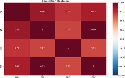
Figure 1 below provides all the variables that are concentrated in the empirical analysis. The heatmap displays that the variable FDI Inflows has a positive association with all the independent variables, with broad money showing the highest correlation. The terms capital formation and broad money also have a significant positive association. However, the correlation does not indicate any inconsistency among the variables.

Figure 1. Correlations Heatmap.

This study utilized secondary time series data that spans the years 1972 to 2021 to assess the impact. Table 2 displays the information about the variables. The reporting economy’s direct investment equity flows are made up of FDI, which includes both equity capital and reinvested profits and other capital. The government of Bangladesh provides incentives for investing under its industrial policy and export-oriented economic plan, with limited legal barriers between international and indigenous private investors. In February 2018, the Bangladeshi Parliament approved the “One Stop Service Bill 2018” with the aim of streamlining the registration processes for investments and businesses involving four “IPAs—Bangladesh Economic Zones Authority (BEZA)‘ is in charge of overseeing special economic zones on the nation’s territory; ’Bangladesh Investment Development Authority (BIDA)‘ is in charge of assisting foreign investors in setting up business in the country; ’Bangladesh Export Processing Zone (BEPZA)‘ is in charge of managing the various export processing zones in Bangladesh; and ’Bangladesh Hi-Tech Park Authority (BHTPA)” is in charge of managing and operating technology business parks throughout the entire country. Bangladesh, a nation that actively seeks FDI, has only garnered a small amount of FDI in the twenty-first century compared to other Asian countries. Furthermore, compared to Bangladesh, FDI inflows per capita have expanded dramatically in populous countries like China, India, and Indonesia (Investment Policy Review, 2013). As seen from previous studies, variables related to ICT development are used to observe FDI inflows in Asia-Pacific countries (Sinha & Sengupta, 2022). In order to investigate the impact on FDI in Pakistan, broad money (M1) is employed as a significant variable (Hina & Anayat, 2019). In this dissertation (Kim, 2018), I tried to find out how the United States’ labor market affects the potential sources of foreign funding that are relevant. This study found a research gap in South Asian countries such as Bangladesh addressing labor markets and capital effects on FDI.

Table 2. Variables details

Variables name	Short form	Log Form	Variable Dimension
Foreign Direct Investment	FDI	LFDI	Dependent Variable
Broad Money (Money circulation)	BM	LBM	Independent Variables
Gross Capital Formation	GCF	LGCF
Technology (Fixed Telephone Subscription)	TEC	LTEC

Sources: WDI, 2023, IFS, 2023.

3.2. Model description and model specification

It is imperative to ascertain whether the variable data is stationary or non-stationary in order to move forward with this study, as the results of the unit root test, which establishes the stationarity of the variable, form the primary basis for choosing the appropriate technique in time series analysis. If all relevant variables exhibit stationarity, the process is simple and allows for the generation of unbiased estimates through vector autoregressive (VAR) modeling. The first difference may also be used to convert non-stationary variables into stationary ones. However, the econometric model is specified as:

(1) $FD{I}_t=\alpha +{\beta }_{1}GC{F}_t+{\beta }_{2}TE{C}_t+{\beta }_{3}B{M}_t+e_t$(1)

Log form of this model is presented in equation number 2.

(2) $LFD{I}_t=\alpha +{\beta }_{1}LGC{F}_t+{\beta }_{2}LTE{C}_t+{\beta }_{3}LB{M}_t+e_t$(2)

Where, $\alpha$ is intercept term, $e_t$ error term, t indicates time and${\beta }_{1,\hspace{0.17em}}\hspace{0.17em}{\beta }_2$ and ${\beta }_3$ are the coefficients of the variables. When using ordinary least squares or similar methods, non-stationary time series can introduce misleading results because regression tests may suggest a significant relationship between two variables that, in reality, lack any meaningful association. This is known as spurious regression and it occurs because of the non-stationarity of the time series used in the regression model. To overcome these obstacles, Engle and Granger (1987) developed a co-integration testing method to examine the interdependencies between non-stationary variables. This method seeks to determine whether or not two or more variables exhibit a long-term equilibrium connection, in which one variable essentially pulls on the other over time, causing the two to move in lockstep. Various traditional approaches, such as Johansen’s (Johansen, 1991), (Johansen, 1995), Engle-Granger’s (Engle & Granger, 1987), and single equation methods, have been utilized for estimating co-integration, which either require all variables to be of order I(1) or employ historical data to determine the variables that are I(0) and I(1) (1); alternatively, the fully modified OLS or dynamic OLS approaches of Johansen (Johansen, 1991, 1995) and Engle-Granger (Engle & Granger, 1987) have also been employed; however, Pesaran et al. (1999) introduced an ARDL modeling approach as a co-integration technique that overcomes such limitations, allowing for the inclusion of beneficiary variables in the co-integrating relationship, regardless of whether they are I(1) or I(0), without requiring the pre-specification of their order; furthermore, the ARDL method is distinct from previous co-integration estimation techniques as it does not assume equal lag lengths and permits varying lag terms for each variable.

As Johansen and Juselius (Johansen & Juselius, 1990) and Engle and Granger (Engle & Granger, 1987) have shown, the autoregressive distributed lag (ARDL) has several benefits over the model of co-integration. To begin with, it may help pick out whether the variables are level co-integrated, first differences, or a hybrid of the two. Second, this technique is much more suited to identifying the co-integration connection of small sample size data series than more conventional co-integration analysis methodologies. Third, because a portion of the regression in this model is endogenous, the t statistics may be validated by using the bound testing technique, which also provides a realistic and unbiased estimate (Narayan, 2005). Fourth, this model uses the right number of delays to provide the targeted framework for modeling (Laurenceson & Chai, 2003) and the fifth point is that the ECM method may be copied from ARDL by doing straightforward linear remodeling (Pesaran et al., 1999).

3.2.1. Augmented Dickey–fuller (ADF) unit root test

Traditionally, stationary variables have been employed to test the hypothesis of co-integration between time series. To ensure the time series variables are stationary, a unit root test is often performed. The ADF test is used to check the hypothesis that the variables are stationary in this research. Generalized by Dickey and Fuller, the ADF test is compatible with higher-order autoregressive dynamics (Dickey & Fuller, 1981). In this case, rendering as white noise using an AR (1) method is inadequate. Augmented Dickey-Fuller’s null hypothesis is:

(3) $H_0:\delta =0$(3)

(4) $H_0:\delta <0$(4)

The following regression model:

(5) $\mathrm{\Delta }{Y}_t={\alpha }_0+Y_{t-1}+{\theta }_i{\sum }_{i=1}^m\mathrm{\Delta }{Y}_{t-1}+{\in }_t$(5)

The optimal lag duration in the dependent variable is m when the initial difference operator is $\mathrm{\Delta }{Y}_{t-1}=\mathrm{\Delta }{Y}_t-\mathrm{\Delta }{Y}_{t-1}$ and the white noise error term is ${\in }_t$ according to the AIC or SC criteria. The best lag duration may be determined with the use of the data dependence approach, which has specific statistical qualities that are favorable for testing the unit root. The data series will be non-stationary and include a unit root if the $H_0$ is not rejected. The data series is stationary and does not have a unit root if the null hypothesis $H_0$ is not accepted. If $Y_t$is stationary with respect to a deterministic linear time trend, then the trend, t i.e., must be included to the set of explanatory variables together with the total number of observations. The Equation can also be written alternatively as:

(6) $\mathrm{\Delta }{Y}_t={\alpha }_0+{\beta }_{0}t+\delta Y_{t-1}+{\theta }_i{\sum }_{i=1}^m\mathrm{\Delta }{Y}_{t-1}+{\in }_t$(6)

The OLS t statistic for testing $\delta =0$ provides the ADF statistics, where $Y_t$represents a random walk with drift around a stochastic trend, and ${\beta }_0$ is the unknown coefficient.

3.2.2. Error correction models

If the variables are I(1) and there is a co-integration relationship, then an error correction model (ECM) may be was conducted. The next link is bivariate; consequently, keep that in the account.

(7) $Y_t=\mu +{\beta }_1{X}_t+{\in }_t$(7)

Using the representation theorem of Engle and Granger (1987), we establish a link between the co-integration and ECM by transforming Eq.

Co-integration equation between $Y_t$ and $X_t$ are as follows:

(8) ${\in }_t=Y_t-\mu -{\beta }_1{X}_t$(8)

The error correction model for $Y_t$, and $X_t$ are as follows:

(9) $\mathrm{\Delta }{Y}_t={\mu }_Y+{\alpha }_Y{\in }_{t-1}+{\sum }_{h=1}^1{a}_{1h}\mathrm{\Delta }{Y}_{t-h}+{\sum }_{h=1}^1{b}_{1h}\mathrm{\Delta }{Y}_{t-h}+u_{Yt}$(9)

(10) $\mathrm{\Delta }{X}_t={\mu }_X+{\alpha }_X{\in }_{t-1}+{\sum }_{h=1}^l{a}_{2h}\mathrm{\Delta }{Y}_{t-h}+{\sum }_{h=1}^l{b}_{2h}\mathrm{\Delta }{X}_{t-h}+u_{Xt}$(10)

Where $u_{Yt}$ and $u_{Xt}$ are white noise processes with a fixed latency of l. The same method may be used to improve the model for the multivariate situation.

3.2.3. ARDL Model

Since the Johansen co-integration test presupposes that all the variables are I(1), it cannot be employed directly if the relevant variables have mixed integration orders or are all stationary. Autoregressive distributed lag (ARDL) model that may be used for non-stationary and mixed-order integration time series. There are enough delays in this model to accurately portray the time it takes for data to be generated. The error correction model (ECM) in dynamic systems may be transformed from ARDL through a linear transformation. Similarly, the ECM gets around problems like misleading associations due to non-stationary time series data by fusing the two without sacrificing any long-run information. To illustrate the ARDL modeling approach, the following simple model can be considered:

(11) $y_t=\alpha +\beta x_t+\delta z_t+e_t$(11)

The error correction version of the ARDL model is given by:

(12) $\mathrm{\Delta }{y}_t={\alpha }_0+{\sum }_{i=1}^p{\beta }_i\mathrm{\Delta }{y}_{t-i}+{\sum }_{i=1}^p{\delta }_i\mathrm{\Delta }{x}_{t-i}+{\sum }_{i=1}^p{\epsilon }_i\mathrm{\Delta }{z}_{t-i}+{\lambda }_1{y}_{t-1}+{\lambda }_2{x}_{t-1}+{\lambda }_3{z}_{t-1}+u_t$(12)

The first component of the equation, denoted by $\beta ,\delta$ and $\epsilon$, describes the short-term behavior of the model. Long-term connection is represented by the second portion after the $\lambda$s. If ${\lambda }_1+{\lambda }_2+{\lambda }_3=0$, then there is no long-term link, which is the null hypothesis in the equation.

3.2.4. Granger causality

The Granger causality test looks at how much of a head start one variable has in predicting another. According to Granger causality, prior values of X1 should provide information that assists in forecasting X2 beyond that offered by past values of X2 alone if a signal X1 Granger-causes (or G-causes) a signal X2. It is mathematically formulated using linear regression and stochastic process modeling (Granger, 2008).

4. Result analysis and discussion

This study’s dependent variable is foreign direct investment (FDI), which is modulated by a wide range of external variables, such as broad money, gross capital formation, and technology (fixed telephone subscription, TEC). FDI denotes the volume of foreign investment in a nation; BM (broad money) is the amount of total money in circulation; GCF is the amount of total fixed asset investment; and TEC is the extent of the country’s technological infrastructure, specifically the number of fixed telephone subscriptions. These variables are studied so that the factors that influence FDI in the economy can be understood and the relationship between FDI and the independent variables can be determined.

Data patterns and outliers may be better understood with summary statistics, which offer an in-depth analysis of the variation and distribution of variables. In this research, three independent variables—broad money (BM), gross capital formation (GCF), and technology (fixed telephone subscription)—are analyzed in connection to foreign direct investment (FDI). The mean FDI is 17.73, and the standard deviation is 3.052, according to Table 3. The smallest FDI value is 11.41, and the highest is 21.76. Broad money has a mean value of 26.95, a standard deviation of 2.229, a minimum value of 23.34, and a high value of 30.54. The standard deviation for GCF is 2.181 (ranging from 21.30 to 30.02), while the mean value is 26.56. Last but not least, the average TEC is 0.390, and the SD is 0.283. The range of possible TEC values is from 0.0701 to 0.932.

Table 3. Summary statistics

	(2)	(3)	(4)	(5)
Variables	Mean	Sd	Min	Max
LFDI	17.73	3.052	11.41	21.76
LBM	26.95	2.229	23.34	30.54
LGCF	26.56	2.181	21.30	30.02
TEC	0.390	0.283	0.0701	0.932

Table 4 displays the eigenvectors or loadings resulting from a principal component analysis (PCA) conducted on a dataset. PC 1 captures the most significant variation in the data and is likely associated with a general factor that combines variables LBM, LGCF, LFDI, and, to a lesser extent, TEC in a positive manner. PC 2 represents a dimension where there is a trade-off between LBM and LGCF, with a larger change in one variable resulting in a smaller change in the other. Additionally, TEC has a strong positive influence on PC 2, while LFDI has a weak negative contribution. PC 3 primarily captures the variation related to LFDI, suggesting a specific factor associated with that variable, while LBM and LGCF have moderate negative associations with PC 3. PC 4 captures the variation primarily driven by LFDI, with a secondary contribution from LGCF and LBM, indicating a specific factor combining these variables. PC 5 captures a more complex relationship among all variables, with LGCF playing a prominent role and LBM exhibiting a strong inverse relationship. TEC has a minor positive association with PC 5, while LFDI has a weak positive influence.

Table 4. Principal component analysis

Eigenvectors (loadings):
Variable	PC 1	PC 2	PC 3	PC 4	PC 5
LFDI	0.444981	−0.011883	0.882926	0.149193	0.005774
LBM	0.460018	−0.264113	−0.303228	0.427220	−0.666456
LGCF	0.457050	−0.341824	−0.280482	0.241112	0.733114
TEC	0.406375	0.886404	−0.203746	0.061939	0.061627

In Table 5, we can see the outcomes of a unit root test applied to LFDI, LBM, LGCF, and TEC. The stationarity qualities of the variables are determined using the ADF (Augmented Dickey-Fuller) test and the KPSS (Kwiatkowski-Phillips-Schmidt-Shin) test. For LFDI, both the ADF and KPSS tests indicate that the variable is stationary at the first difference (I(1)), as evidenced by the significantly negative test statistics (−5.522 for ADF and −4.523 for KPSS). Similarly, for LBM and LGCF, both tests suggest that these variables are stationary at the first difference (I(1)). The ADF and KPSS test statistics for LBM are 2.195 and −3.380, respectively, while for LGCF, they are −1.518 and −6.921. On the other hand, TEC exhibits different results. The ADF test indicates that TEC is stationary at the level (I(0)) with a test statistic of −3.052, suggesting the absence of a unit root. However, the KPSS test indicates some level of stationarity at the first difference (I(1)), with a test statistic of −3.712.

Table 5. Unit root test

Variable	ADF Test		KPSS Test		Remark
	Level	1^st Diff.	Level	1^st Diff.
LFDI	−0.055	−5.522***	−1.431	−4.523***	Stationary at I(1)
LBM	2.195	−3.380***	1.811	−7.319***	Stationary at I(1)
LGCF	−1.518	−6.512***	−1.491	−6.921***	Stationary at I(1)
TEC	−3.052**		−3.7121**		Stationary at I(0)

The Zivot-Andrews (ZA) unit root test was used to analyze structural breaks for LFDI, LBM, LGCF, and TEC, and the findings are shown in Table 6. Time series data may be analyzed for structural breakdowns using the ZA statistic. For LFDI, the ZA statistic is −3.088, indicating the presence of a structural break in the data. The break is identified as having occurred in 1997. At the 1%, 5%, and 10% levels, the critical values are −5.34, −4.93, and −4.58, respectively. Based on the ZA statistic and the critical values, it can be concluded that a structural break exists in LFDI. Similarly, for LBM and LGCF, the ZA statistics are −3.784 and −4.114, respectively. These esteemed values insinuate the existence of opulent structural breaks in the corresponding variables. The breaks are identified to have occurred in 1989 and 1991 for LBM and LGCF, respectively. For TEC, the ZA statistic is −3.11, indicating a potential structural break in the data. The break is identified as having occurred in 2001.

Table 6. Structural breaks (ZA unit root test)

Variables	ZA statistic	Break	1%	5%	10%	Decision
LFDI	−3.088***	1997	−5.34	−4.93	−4.58	Break Exist
LBM	−3.784***	1989	−5.34	−4.93	−4.58
LGCF	−4.114**	1991	−5.34	−4.93	−4.58
TEC	−3.11*	2001	−5.34	−4.93	−4.58

Note: The significance levels are denoted as *** for 1%, ** for 5%, and * for 10%.

Table 7, showcasing the exquisite findings of the optimal lag selection for a most refined and sophisticated model The lag column specifies the number of lags considered in the model, while the remaining columns provide various evaluation criteria for each lag. The Log Likelihood (LogL) metric denotes the maximum value attained by the likelihood function, which implies an improved alignment of the model with the data as the metric value rises. The LR (Likelihood Ratio) statistic measures the model’s overall fit relative to a restricted model with fewer lags, and higher values suggest a significantly improved fit. The FPE (Final Prediction Error) criterion assesses the accuracy of the model’s predictions, with smaller values indicating better predictive performance. The AIC (Akaike information criterion) balances the model’s goodness of fit and complexity, with lower values indicating a superior trade-off between fit and complexity. The Schwarz criterion (SC), which is also referred to as the Bayesian information criterion (BIC), follows a similar approach to AIC in that it penalizes models with additional parameters more severely. A smaller value of SC is indicative of a superior trade-off between model fit and complexity. Lastly, the HQ (Hannan-Quinn criterion) criterion is another measure of model selection that considers both appropriateness and complexity, with smaller values implying a more favorable balance. The selection of the optimal lag length is based on various criteria, such as LogL, LR, FPE, AIC, SC, and HQ values. The chosen lag length is the one that provides the most favorable balance between model fit and complexity.

Table 7. Optimal lags selection

Lag	LogL	LR	FPE	AIC	SC	HQ
0	−119.3404	NA	0.009238	6.667050	6.841203	6.728447
1	94.85615	370.5022*	2.07e-07*	−4.046279*	−3.175512*	−3.739293*
2	107.5433	19.20219	2.56e-07	−3.867206	−2.299827	−3.314632
3	121.5198	18.13161	3.11e-07	−3.757825	−1.493832	−2.959662

*Indicates 5% level of significance.

Table 7 denotes statistical significance at the 5% level through the use of asterisks (*). The statistical significance of Lag 1 can be inferred from the AIC and SC values, which are −4.046279 and −3.175512, respectively. These values suggest that Lag 1 is statistically significant at the 5% level. The analysis of the given criteria indicates that Lag 1 is the most suitable lag length, as it produces the highest LogL value and lower values for FPE, AIC, SC, and HQ in comparison to other lag lengths. This implies that Lag 1 exhibits the optimal balance between the adequacy of the model and its intricacy.

Table 8 presents the results of the bound co-integration test, a statistical method used to determine the presence of a long-term relationship between two or more variables in an autoregressive distributed lag (ARDL) model. The determined value of the test statistic, which is 2.929, is displayed in the test statistic column. The value column displays the K, or 3 in this case, number of incorporated delays in the test. The optimal lag for the model is 1. The section titled Critical Value Bounds contains the critical values corresponding to different levels of significance, namely 10%, 5%, and 1%. The values for I(0) and I(1) are provided to indicate the presence or absence of co-integration in the given situations. At a significance level of 10%, the critical value boundaries for I(0) and I(1) are 2.45 and 3.52, respectively. At a 5% significance level, the critical value boundaries for I(0) and I(1) are 2.86 and 4.01, respectively. At a significance level of 1%, the critical value boundaries for I(0) and I(1) are 3.74 and 5.06, respectively. The obtained F-statistic value of 2.929 surpasses the significance thresholds for all levels, namely 5% and 10%. The aforementioned indicates a persistent association between the variables, thereby leading to the rejection of the null hypothesis that posits the absence of co-integration between them.

Table 8. Bound co-integration test

Test Statistic	Value	K
F- Statistic	2.929	3
Critical Value Bounds
Significance level	I(0)	I(1)
10%	2.45	3.52
5%	2.86	4.01
1%	3.74	5.06

The results of an ARDL analysis are displayed in Table 9, which exhibits the coefficients, standard errors, t-statistics, and probabilities pertaining to each variable included in the model. The results shed substantial insight into the interrelationships between the aforementioned predictors and outcome factors. The estimated coefficient of determination for the variable LFDI(−1) is positive, at 0.72. There is strong statistical significance for the coefficient at the 1% level, indicating that the delayed variable has a large impact on the dependent variable. The estimated coefficient of 4.36 for the variable LGCF indicates a positive association, which is significant at the 1% level of significance. There is a positive association between FDI and capital formation, as founded by Rahman (2023). In contrast, LGCF (−1) demonstrates a negative association, as evidenced by a coefficient estimate of −3.53, which is likewise significant at the 1% level of statistical significance. The estimated coefficient of −6.76 for the variable designated as “LBM” indicates a statistically significant negative association at the 1% level of significance. Similarly, there is a positive connection between delayed LBM (−1) and all other variables, with an estimated value of 5.88 that is significant at the 1% level. In addition, the LTEC variable is positively correlated, as shown by a coefficient estimate of 1.55, which is statistically significant at the 1% level. Technological advancement increase the FDI which findings is supported by (Qamruzzaman & Kler, 2023; Rahman et al., 2023) The substantial impacts of the aforementioned factors on the dependent variable are highlighted, with support from statistically significant t-statistics. Although the constant term C displays a positive correlation with the dependent variable, the absence of statistical significance at conventional levels implies that its effect may not be substantial. The R-square value of 0.93 is indicative of a strong fit of the model, explaining about 93% of the variation in the dependent variable. The adjusted R-square value of 0.91 is a more cautious estimate of the model’s explanatory capacity, given the quantity of predictors. The standard error of the regression, which has been quantified as 0.87, serves as an estimation of the mean discrepancy between the predicted and observed values. This metric is indicative of the precision of the model in approximating the dependent variable. The calculation of the sum squared residual of 26.98 is indicative of the total sum of squared differences between the predicted and observed values. The log-likelihood function is a statistical measure that provides an estimation of the probability of the observed data given the model’s parameters. In this case, the log-likelihood value of −50.99 represents the aforementioned function. The statistical analysis reveals that the model’s overall significance is indicated by the F-statistic of 74.93, which is further supported by a p-value of 0.00. In addition, the Durbin-Watson statistic of 2.06 indicates the lack of significant autocorrelation in the residuals, as a value in proximity to 2 denotes the absence of substantial autocorrelation.

Table 9. ARDL output

Variable	Coefficient	Std. Error	t-Statistic	Prob.*
LFDI(−1)	0.72	0.10	6.99	0.00
LGCF	4.36	1.66	2.62	0.01
LGCF(−1)	−3.53	1.11	−3.19	0.00
LBM	−6.76	2.53	−2.67	0.01
LBM(−1)	5.88	2.26	2.60	0.01
LTEC	1.55	0.58	2.69	0.01
C	8.76	6.02	1.46	0.15
R-square	0.93
Adjusted R-square	0.91
S.E. of regression	0.87
Sum squared resid	26.98
Log likelihood	−50.99
F-statistic	74.93
Prob(F-statistic)	0.00
Durbin-Watson stat	2.06

The dynamics of the model in both the short and long run are presented in Table 10. The short-term dynamics or co-integrating form displays the coefficients, standard errors, t-statistics, and probabilities for each variable. The coefficient of the variable D (LGCF) is 4.36, accompanied by a standard error of 1.66, which suggests a positive correlation. The statistical significance of the t-statistic at the 1% level is indicated by its t-statistic value of 2.62. The coefficient of the variable D (LBM) is −6.76 with a standard error of 2.53, indicating a negative correlation. The statistical significance of the t-statistic, which has a value of −2.67, is established at the 1% level. With a coefficient of 1.55 and a standard error of 0.58, the variable D (LTEC) indicates a positive connection supported by Majumder and Rahman (2020). The t-statistic of 2.69 confirms the significance of the aforementioned finding at the 1% level of significance. Majumder et al. (2022) and Majumder et al. (2022) have supported the findings that technology and FDI have a positive relationship. With a coefficient of −0.28 and a standard error of 0.10, the CointEq(−1) variable is negative and significant, meaning that the speed of adjustment (28%), which has a t-statistic of −2.72, is statistically significant at the 1% level of confidence. The equation for co-integration is expressed as:

Table 10. Short and Long Run Dynamics

Short Run Dynamics or Co-integrating Form
Variable	Coefficient	Std. Error	t-Statistic	Prob.
D(LGCF)	4.36	1.66	2.62	0.01
D(LBM)	−6.76	2.53	−2.67	0.01
D(LTEC)	1.55	0.58	2.69	0.01
CointEq(−1)	−0.28	0.10	−2.72	0.01
Cointeq = LFDI - (2.9669*LGCF −3.1289*LBM + 5.5434*LTEC + 31.2393)
Long Run Coefficients
LGCF	2.97	2.96	1.00	0.32
LBM	−3.13	3.10	−1.01	0.32
LTEC	5.54	2.60	2.13	0.04
C	31.24	25.21	1.24	0.22

Cointeq = LFDI - (2.9669LGCF–3.1289LBM +5.5434*LTEC +31.2393).

Coefficients, standard errors, t-statistics, and probabilities are all shown in Table 10 for each variable across time. The coefficient of the LGCF variable in the regression analysis is 2.97, and its standard error is 2.96. There seems to be a favorable relationship between the two factors. With a t-value of 1, it is not statistically significant at the most basic level of analysis. The coefficient of LBM in the regression analysis is −3.13, which implies an inverse relationship. The coefficient’s standard error is 3.10. A t-statistic of −1.01 indicates a result that is not statistically significant. The coefficient of LTEC in the regression analysis is 5.54 with a standard error of 2.60, indicating a statistically significant positive relationship. The t-statistic of 2.13 is significantly different from zero at the 5% level of significance. The constant term’s coefficient (denoted by C) is 31.24 with a standard error of 25.21, which is statistically significant in favor of a positive impact. A t-value of 1.24, which is shows that the impact being seen is not statistically significant at the typically used levels of significance. Examining the probabilities associated with each coefficient might shed light on their statistical importance.

Checking for residual correlation and heteroskedasticity in the model is part of the residual diagnostics test, the results of which are shown in Table 11 below. To test whether or not the residuals exhibit serial correlation, the Breusch-Godfrey Serial Correlation LM Test is used. A probability of 0.50 is assigned to the calculated F-statistic value of 0.72 (Prob. F(2,34)). Based on these findings, it seems that there is little evidence to support the hypothesis of serial correlation in the residuals. A lack of serial correlation is further supported by the low likelihood (Prob. Chi-Square (2)) and low value (Obs. R-squared) of 0.42. The Heteroskedasticity Test recommends using the Breusch-Pagan-Godfrey test to determine whether or not the residuals exhibit heteroskedasticity. The associated probability (Prob. F(6,36)) is 0.15, and the related F-statistic value is 1.71. Based on these findings, it seems that heteroskedasticity is not present. There is no heteroskedasticity, as shown by the Obs. R-squared value of 9.54 and the probability (Prob. Chi-Square (6)) of 0.15 found by the statistical analysis. Additionally, the probability (Prob. Chi-Square (6)) associated with the scaled explained sum of squares is 8.78. This result further substantiates the absence of heteroskedasticity.

Table 11. Residual diagnostics tests

Breusch-Godfrey Serial Correlation LM Test: H0= No serial Correlation
F-statistic	0.72	Prob. F(2,34)	0.50
Obs*R-squared	1.74	Prob. Chi-Square(2)	0.42
Heteroskedasticity Test: Breusch-Pagan-Godfrey: H0= No Heteroskedasticity
F-statistic	1.71	Prob. F(6,36)	0.15
Obs*R-squared	9.54	Prob. Chi-Square(6)	0.15
Scaled explained SS	8.78	Prob. Chi-Square(6)	0.19

Figure 2 shows the Cumulative Sum (CUSUM) and Cumulative Sum of Squares (CUSUMsq) stability tests. The tests were 5% significant. The CUSUM test uses the cumulative sum of recursive residuals to detect substantial stability deviations over time. The model is unstable if the CUSUM test statistic exceeds critical bounds at 5% significance. The CUSUMsq test uses the cumulative sum of squared recursive residuals to assess model stability. In the event that the CUSUMsq test statistic exceeds the critical bounds at a significance level of 5%, it indicates an absence of stability in the model. The stability test outcomes reveal that, at a 5% significance level, the critical bounds are not surpassed by either the CUSUM test or the CUSUMsq test. The aforementioned observation implies the absence of substantial indications of instability or alterations in the model’s structure throughout the course of time. Moreover, the outcomes of the Granger causality analysis, which investigated the causal connections among different variables, are displayed in Table 12. The assessment examines the extent to which a given variable serves as a Granger cause for another variable, thereby indicating the degree to which the former variable contributes valuable insights for forecasting the latter variable. Results from the tests show that LGCF does not display Granger causality towards LFDI. A likelihood of 0.29 and an F-statistic of 1.16 both indicate that there is insufficient data to draw conclusions about a cause-and-effect connection between LGCF and LFDI. With an F-statistic of 1.63 and a likelihood of 0.21, it is clear that there is insufficient evidence to conclude that LFDI is a Granger cause of LGCF. In addition, the evaluation takes a close look at the correlations between LBM and LTEC and the other factors. Based on the substantial F-statistic of 4.62 and the probability value of 0.04, the research concludes that there is a bidirectional causal link between LBM and LFDI. In contrast, an F-statistic of 4.48 and a probability value of 0.04 shows that LFDI does not show Granger causality with LBM. In addition, an F-statistic of 4.07 and a probability value of 0.05 indicate that LTEC displays unidirectional Granger causality towards LFDI. Concurrently, the likelihood of a link between LFDI and LTEC is rather high at 0.59, and the F-statistic is quite small at 0.30. The results of the Granger causality test suggest that LBM and LGCF are causally related to one another, which is supported by Rahman (2023). The statistical study shows that LBM had no effect on LGCF (F-statistic = 74.61, p = .00). This shows a strong causal relationship between the variables. The F-statistic of 13.42 and probability value of 0.00 indicate a strong causal link between LGCF and LBM. The experiment proves LGCF produces LBM. LTEC’s F-statistic of 2.04 and the likelihood of 0.16 reveal no Granger causation toward LGCF. LGCF is not the cause of LTEC. LBM causes LTEC, according to the findings (F-statistic 3.37, a probability of 0.07). The Granger causality test proves LTEC causes LBM. The consistent conclusion of the findings is that capital formation and technology have a positive impact on FDI; on the other hand, money circulation has a negative impact on FDI in Bangladesh.

Figure 2. Stability test: CUSUM and CUSUMsq tests.

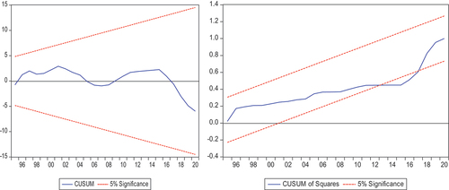
Table 12. Granger causality test

Null Hypothesis:	F-Statistic	Prob.	Decision
LBM ≠ LFDI	4.62	0.04	Bidirectional
LFDI ≠ LBM	4.48	0.04
LGCF ≠ LFDI	1.16	0.29	No causality
LFDI ≠ LGCF	1.63	0.21
LTEC ≠ LFDI	4.07	0.05	Unidirectional
LFDI ≠ LTEC	0.30	0.59
LBM ≠ LGCF	74.61	0.00	Bidirectional
LGCF ≠ LBM	13.42	0.00
LTEC ≠ LGCF	2.04	0.16	Unidirectional
LGCF ≠ LTEC	3.01	0.09
LTEC ≠ LBM	3.37	0.07	Unidirectional
LBM ≠ LTEC	1.99	0.17

Note: The symbol “≠” refer the statement of null hypothesis assumption “does not Granger cause.”

5. Conclusion and recommendations

This study’s goal was to learn more about how capital, technology development, and general money affect a country’s foreign direct investment in order to better understand how those elements affect the economy. While determining how capital formation and technological advancement affect FDI in Bangladesh are the main goals, it is also important to consider whether money circulation has a positive or negative impact on FDI. This study has used time series data from 1972–2021 and several preliminary tests, such as the unit root, structural break, and cointegration test. The result of the unit root test indicates an ARDL model because of stationarity at levels I(0) and I(1). Key findings of this result estimation show that, to estimate the cointegration, the calculated F-statistic value of 2.929 exceeds the 5% and 10% significance limits for all levels. The null hypothesis, which states that there is no co-integration between the variables, is rejected because the aforementioned data show a persistent connection between the variables. At the 1% level of significance, the calculated coefficient of the variable LGCF shows a positive value to explain FDI. At the 1% level of significance, the calculated coefficient for the variable labeled LBM shows a statistically significant and negative effect on FDI. The circulation of money (broad money) has a negative impact on FDI in Bangladesh. The negative impact of LBM deals with the expansion of inflation, which reduces the money supply and induces FDI. Additionally, a coefficient estimate of 1.55, which is statistically significant at the 1% level, demonstrates the LTEC variable’s positive correlation. The CointEq(−1) or ECT variable has a −0.28 coefficient, which shows the level of adjustment at a speed of 28% towards equilibrium. A consistent result was also estimated for the long run, where the coefficients of the variables LTEC and LGCF are positive and LBM is negative, to explain DFI in Bangladesh. Causality shows there is bidirectional causality between FDI and money circulation, unidirectional causality between technology and FDI, bidirectional causality between money circulation and capital formation, and unidirectional causality between technology and capital formation.

Based on its findings, this study pursues several policies that can increase FDI flow in Bangladesh. Foreign direct investment (FDI) can be greatly increased in Bangladesh by capital formation and technological advancement, as this study found a positive impact on FDI, which is supported by economic theory. Investments are made in infrastructure projects, including power generation, telecommunications networks, and transportation networks. For foreign investors, a more business-friendly environment with improved infrastructure means fewer logistical and operational difficulties. Bangladesh may become a more appealing location for FDI by upgrading its ports, highways, and other transportation infrastructure. This will improve connectivity and ease the movement of products and services. Initiatives for skill development and education can benefit from capital formation. Bangladesh can create a qualified workforce that satisfies the demands of international investors by investing in high-quality education and vocational training. A well-educated and trained workforce enhances productivity and competitiveness, making the country an appealing location for FDI. Foreign investors are more likely to invest in a country where they can find a talented and capable workforce. This study discovered a strong correlation between technological advancement and FDI, demonstrating how important technology growth is to luring FDI. Research and development projects, innovation hubs, and technology parks can all benefit from capital formation. Encouragement of technological development can lead to the development of cutting-edge goods, services, and procedures, luring in international investors looking for access to cutting-edge technology. Bangladesh is a desirable location for FDI due to its emphasis on sectors like information technology, software development, and telecommunications, which can promote innovation and technical growth. In Bangladesh, SEZs can be created and developed through capital formation. To entice international investors, these zones provide a variety of incentives, including tax advantages, streamlined regulatory processes, and infrastructure facilities. Bangladesh can create a welcoming investment environment and attract FDI inflows by investing in the development of SEZs. To attract FDI, the government must be dedicated to enacting reforms and policies that benefit investors. The creation of capital can be used to make business environments better, make rules simpler, and increase transparency. These actions maintain trust among international investors and foster a steady and predictable investment environment. FDI inflows to Bangladesh can be greatly increased by a supportive policy environment that encourages ease of doing business. Bangladesh may increase its allure as a location for investment by concentrating on capital formation, infrastructural development, human capital development, technological breakthroughs, and enacting beneficial legislation. These elements help to create an environment that is favorable for foreign investors, luring them to the nation and fostering economic growth and development. Further study would include considering other macroeconomic variables such as labor, human resources, and energy issues.

Disclosure statement

No potential conflict of interest was reported by the authors.

Data availability statement

Data will be available based on request.

Additional information

Funding

This work was supported by the Universitas Airlangga [NA].

References

- Adeleye, N., & Eboagu, C. (2019). Evaluation of ICT development and economic growth in Africa. NETNOMICS: Economic Research and Electronic Networking, 20, 31–23. https://doi.org/10.1007/s11066-019-09131-6
- Ahmad, H., Shafiq, N., & Hassan, S. (2015). Research article examine the effects of money supply M1 and gdp on fdi in Pakistan. International Journal of Current Research, 7(3), 13498–13502.
- Ahmed, M. U., Muzib, M. M., & Saha, S. (2015). The money supply process in Bangladesh: An Econometric analysis. Global Disclosure of Economics and Business, 4(2), 137–142. https://doi.org/10.18034/gdeb.v4i2.142
- Akbas, Y. E., Senturk, M., & Sancar, C. (2013). Testing for causality between the foreign direct investment, current account deficit, GDP and total credit: Evidence from G7. Panoeconomicus, 60(6), 791–812. https://doi.org/10.2298/PAN1306791A
- Arvin, M. B., Pradhan, R. P., & Nair, M. (2021). Uncovering interlinks among ICT connectivity and penetration, trade openness, foreign direct investment, and economic growth: The case of the G-20 countries. Telematics and Informatics, 60(August 2020), 101567. https://doi.org/10.1016/j.tele.2021.101567
- Bedir, S., & Soydan, A. (2016). Implications of FDI for current account balance: A panel causality analysis. Eurasian Journal of Economics and Finance, 4(2), 58–71. https://doi.org/10.15604/ejef.2016.04.02.005
- Bhujabal, P., & Sethi, N. (2020). Foreign direct investment, information and communication technology, trade, and economic growth in the South Asian Association for Regional Cooperation countries: An empirical insight. Journal of Public Affairs, 20(1), e2010. https://doi.org/10.1002/pa.2010
- Bhujabal, P., Sethi, N., & Padhan, P. C. (2021). ICT, foreign direct investment and environmental pollution in major Asia Pacific countries. Environmental Science and Pollution Research, 28(31), 42649–42669. https://doi.org/10.1007/s11356-021-13619-w
- Dickey, D. A., & Fuller, W. A. (1981). Likelihood Ratio Statistics for Autoregressive Time Series with a Unit Root. http://www.erudito.fea.usp.br/PortalFEA/Repositorio/537/Documentos/DIckey-Fuller(1981).pdf
- Engle, R. F., & Granger, C. W. J. (1987). Co-integration and error correction: Representation. International Journal of Offshore and Polar EngineeringEstimation, 55(2), 251–276. https://doi.org/10.2307/1913236
- Granger, C. W. J. (2008). Investigating causal relations by Econometric models and cross-spectral methods. Essays in Econometrics Vol II: Collected Papers of Clive W J Granger, 37(3), 31–47. https://doi.org/10.1017/ccol052179207x.002
- Hina, M., & Anayat, U. (2019). The role of money supply: Foreign direct investment & economic growth in Pakistan. International Journal of Economics, Commerce and Management, VII(2), 281–289. http://ijecm.co.uk
- Hussain, A., Batool, I., Akbar, M., & Nazir, M. (2021). Is ICT an enduring driver of economic growth? Evidence from South Asian economies. Telecommunications Policy, 45(8), 102202. https://doi.org/10.1016/j.telpol.2021.102202
- Investment Policy Review. (2013).
- Johansen, S.(1991). Estimation and hypothesis testing of cointegration vectors in gaussian vector autoregressive models. Econometrica: Journal of the Econometric Society. https://doi.org/10.2307/2938278
- Johansen, S. (1995). Identifying restrictions of linear equations with applications to simultaneous equations and cointegration. Journal of Econometrics, 69(1), 111–132. https://doi.org/10.1016/0304-4076(94)01664-L
- Johansen, S., & Juselius, K. (1990). Maximum Likelihood Estimation and Inference on Cointegration - With2.
- Kaur, M., Yadav, S., & Gautam, V. (2012). Foreign direct investment and Current account deficit - a causality analysis in context of India. Journal of International Business and Economy, 13(2), 85–106. https://doi.org/10.51240/jibe.2012.2.4
- Kim, E. (2018). The Labor Market Effects of Foreign Direct Investment and Institutional Changes in The United States. ProQuest Dissertations and Theses. University of Pennsylvania. http://cyber.usask.ca/login?url=https://search.proquest.com/docview/2117678111?accountid=14739&bdid=6472&_bd=ybhhgrcXq8ZuoXrHmzqIUwesyX4%3D
- Latifa, Z., Yang, D., Shahid, L., Liu, X., Pathana, Z., Salama, S., Jianqiu, Z., & Jianqiu, Z. (2017). The dynamics of ICT, foreign direct investment, globalization and economic growth: Panel estimation robust to heterogeneity and cross-sectional dependence. Telematics and Informatics, 35(2), 318–328. https://doi.org/10.1016/j.tele.2017.12.006
- Laurenceson, J., & Chai, J. C. H. (2003). Financial reform and economic development in hina. In Syria Studies. https://www.researchgate.net/publication/269107473_What_is_governance/link/548173090cf2525dcb61443/download%0Ahttp://www.econ.upf.edu/~reynal/Civilwars_12December2010.pdf%0Ahttps://think-asia.org/handle/11540/8282%0Ahttps://www.jstor.org/stable/41857625
- Liu, X., & Wang, L. (2019). Predictive analysis of China’s broad money supply (M2) Based on ARIMA-GARCH model. Francis Academic Press, UK, 1–6. https://doi.org/10.25236/etmhs.2019.302
- Majumder, S. C., & Rahman, M. H. (2020). Impact of foreign direct investment on economic growth of China after economic reform. Journal of Entrepreneurship, Business and Economics, 8(2), 120–153.
- Majumder, S. C., Rahman, M. H., & Martial, A. A. A. (2022). The effects of foreign direct investment on export processing zones in Bangladesh using generalized method of moments approach. Social Sciences & Humanities Open, 6(1), 100277. https://doi.org/10.1016/j.ssaho.2022.100277
- Mohammed Ershad, H., & Mahfuzul, H. (2017). Empirical analysis of the relationship between money supply and per capita GDP growth rate in Bangladesh. Journal of Advances in Economics and Finance, 2(1). https://doi.org/10.22606/jaef.2017.21005
- Mwakabungu, B. H. P., & Kauangal, J. (2023). An empirical analysis of the relationship between FDI and economic growth in Tanzania. Cogent Economics & Finance, 11(1), 2204606. https://doi.org/10.1080/23322039.2023.2204606
- Narayan, P. K. (2005). The saving and investment nexus for China: Evidence from cointegration tests. Applied Economics, 37(17), 1979–1990. https://doi.org/10.1080/00036840500278103
- Norehan, M. A. H. B., Ridzuan, A. R. B., & Ismail, S. B. (2021). Conceptual framework for ICT development and foreign direct investment inflows as drivers for sustainable economic growth: Evidence from China and Malaysia. International Journal of Academic Research in Economics and Management Sciences, 10(1), 123–134. https://doi.org/10.6007/ijarems/v10-i1/9631
- Nunnenkamp, P. & Spatz, J. (2002). Determinants of fdi in developing countries: Has globalization changed the rules of the game? by determinants of fdi in developing countries: has globalization changed the rules of the game ? Transnational Corporations, 11(2), 1–34. http://hdl.handle.net/10419/2976
- Ogundipe, A. A., Oye, Q. E., Ogundipe, O. M., Osabohien, R., & Andraz, J. M. L. G. (2020). Does infrastructural absorptive capacity stimulate FDI-Growth nexus in ECOWAS? Cogent Economics & Finance, 8(1), 1751487. https://doi.org/10.1080/23322039.2020.1751487
- Pesaran, M. H., Pesaran, M. H., Shin, Y., & Smith, R. P. (1999). Pooled mean group estimation of dynamic heterogeneous panels. Journal of the American Statistical Association, 94(446), 621–634. https://doi.org/10.1080/01621459.1999.10474156
- Pradhan, R. P., Arvin, M. B., Hall, J. H., & Bennett, S. E. (2018). Mobile telephony, economic growth, financial development, foreign direct investment, and imports of ICT goods: The case of the G-20 countries. Economia e Politica Industriale, 45(2), 279–310. https://doi.org/10.1007/s40812-017-0084-7
- Pradhan, R. P., Arvin, M. B., Nair, M., Mittal, J., & Norman, N. R. (2017). Telecommunications infrastructure and usage and the FDI–growth nexus: Evidence from asian-21 countries. Information Technology for Development, 23(2), 235–260. https://doi.org/10.1080/02681102.2016.1217822
- Qamruzzaman, M., & Kler, R. (2023). Do Clean energy and financial innovation induce SME performance? Clarifying the nexus between financial innovation, technological innovation, Clean energy, environmental degradation, and SMEs performance in Bangladesh. International Journal of Energy Economics & Policy, 13(3), 313–324. https://doi.org/10.32479/ijeep.14185
- Rahman, M. H. (2023). Does the current account balance influence foreign direct investment in the Indian economy? Application of quantile regression model. SN Business & Economics, 3(5), 94. https://doi.org/10.1007/s43546-023-00471-y
- Rahman, P., Zhang, Z., & Musa, M. (2023). Do technological innovation, foreign investment, trade and human capital have a symmetric effect on economic growth? Novel dynamic ARDL simulation study on Bangladesh. Economic Change and Restructuring, 56(2), 1327–1366. https://doi.org/10.1007/s10644-022-09478-1
- Rao, D. T., Sethi, N., Dash, D. P., & Bhujabal, P. (2023). Foreign aid, FDI and economic growth in South-East Asia and South Asia. Global Business Review, 24(1), 31–47. https://doi.org/10.1177/0972150919890957
- Rehman, A., Ma, H., Ahmad, M. A., Ozturk, I. O., & Işık, C. (2021). Estimating the connection of information technology, foreign direct investment, trade, renewable energy and economic progress in Pakistan: Evidence from ARDL approach and cointegrating regression analysis. Springer Link, 28(36), 50623–50635. https://doi.org/10.1007/s11356-021-14303-9
- Sassi, S., & Goaied, M. (2013). Financial development, ICT diffusion and economic growth: Lessons from MENA region. Telecommunications Policy, 37(4–5), 252–261. https://doi.org/10.1016/j.telpol.2012.12.004
- Sethi, N., Bhujabal, P., Das, A., & Sucharita, S. (2019). Foreign aid and growth nexus: Empirical evidence from India and Sri Lanka. Economic Analysis and Policy, 64, 1–12. https://doi.org/10.1016/j.eap.2019.07.002
- Shahidan, S. M., Angel, E. M., Rahim, R. A., Fadzilah Zainal, N., & Sugiharti, L. (2022). The impacts of corruption and environmental degradation on foreign direct investment: New evidence from the ASEAN+3 countries. Cogent Economics & Finance, 10(1). https://doi.org/10.1080/23322039.2022.2124734
- Sinha, M., & Sengupta, P. P. (2022). FDI inflow, ICT expansion and economic growth: An empirical study on Asia-Pacific developing countries. Global Business Review, 23(3), 804–821. https://doi.org/10.1177/0972150919873839
- Soper, D. S., Demirkan, H., Goul, M., & St Louis, R. (2012). An empirical examination of the impact of ICT investments on future levels of institutionalized democracy and foreign direct investment in emerging societies. Journal of the Association for Information Systems, 13(3), 116–149. https://doi.org/10.17705/1jais.00289
- Wong, M. F., Fai, C. K., Yee, Y. C., & Cheng, L. S. (2019). Macroeconomic policy and exchange rate impacts on the foreign direct investment in ASEAN economies. International Journal of Economic Policy in Emerging Economies, 12(1), 1–10. https://doi.org/10.1504/IJEPEE.2019.098629
- Yang, X., & Shafiq, M. N. (2020). The impact of foreign direct investment, capital formation, inflation, money supply and trade openness on economic growth of Asian countries. IRASD Journal of Economics, 2(1), 25–34. https://doi.org/10.52131/joe.2020.0101.0013
- Zafir, C., & Sezgin, F. (2012). Analysis of the effects of foreign direct investment on the financing of Current account deficits in Turkey. International Journal of Business & Social Science, 03, 1–12. https://www.academia.edu/22541576/Analysis_of_the_Effects_of_Foreign_Direct_Investment_on_the_Financing_of_Current_Account_Deficits_in_Turkey