Determinants of inequalities in welfare among households in Ethiopia: A comparative study of urban and rural Ethiopia

Abstract

This study aims to investigate welfare inequality between households in rural and urban Ethiopia using secondary data obtained from the Living Standards Measurement Surveys (LSMS) available on the World Bank website. The data was analyzed using the Atkinson Index to identify welfare inequality among households and quantile regression to identify determinants of welfare inequality in rural and urban Ethiopia. The results show that the Atkinson index for the rural group is 0.123006, while it is 0.110899 for the urban group, indicating a higher level of welfare inequality in rural areas. Furthermore, the quantile regression analysis reveals that among the factors measured, the number of assets, access to health services, and saving are important determinants of welfare inequality in rural households. On the other hand, the number of livestock and household size are found to be significant factors contributing to welfare inequality in urban areas. This study provides valuable insights into the specific drivers of welfare inequality in both rural and urban settings and can inform policymakers on how to address these inequalities to promote social and economic development in Ethiopia.

Keywords:

• Atkinson Index
• Ethiopia
• inequality
• Lorentz curve
• quantile regression
• social and economic development
• rural and urban
• welfare

PUBLIC INTEREST STATEMENT

This study explores the differences in welfare between urban and rural households in Ethiopia. It reveals a higher level of welfare inequality among rural families, indicating they have fewer resources and services compared to their urban counterparts. The study identifies factors contributing to such disparities, like assets and access to health services in rural areas, and livestock and household size in urban regions. The findings can help officials understand what drives these inequalities, and formulate strategies to bridge this gap. The aim is to boost economic development and social equality across the nation. This research adds to our understanding of the persistent economic imbalances between rural and urban areas not only in Ethiopia but potentially in other developing countries as well.

1. Introduction

Both academic and policy circles have recently shown an increasing interest in the subject of inequality. The concept of inequality is complex as it encompasses various dimensions, including income, wealth, welfare, access to resources and opportunities, and distribution of public goods and services. Knowing the factors that contribute to inequalities in well-being among households is a crucial prerequisite for formulating and executing effective strategies aimed at mitigating the gap between the wealthy and the poor (World Bank, 2016). Worldwide, inequality has been accordingly acknowledged as a major obstacle to accomplishing the United Nations’ Sustainable Development Goals (SDGs), particularly Goal 10, which mandates the reduction of inequalities within and among nations. Therefore, there is a growing focus on understanding the underlying factors contributing to disparities in welfare among households on a national and global scale (United Nations, 2015).

Ethiopia has undergone rapid economic growth and a transition from an agrarian-based economy to a more diversified, urban-centric growth model. Despite the impressive economic growth over the past two decades, a significant gap exists between urban and rural households in terms of welfare outcomes. Generally, urban areas have superior access to basic services, education, healthcare, and employment opportunities. This information is according to the World Bank’s report in 2015. National policy frameworks in Ethiopia have attempted to address inequality through a range of poverty alleviation and social protection programs. The Ethiopian government implemented the Growth and Transformation Plan (GTP) between 2010 and 2015, which aimed to achieve broad-based economic growth and reduce poverty by focusing on human development, infrastructure development, and good governance (Muleta & Belete, 2017). Despite these efforts, regional disparities persist, and understanding the factors that drive these disparities has become vital for planning effective policy interventions. A substantial body of literature exists on the determinants of inequalities in welfare among households, which has identified factors such as income, education, access to basic services, employment opportunities, social safety nets, and demographic factors as significant determinants of welfare disparities between households (Alemu et al., 2018; Korzeniewicz & Moran, 2018).

Moreover, the significant influence of geography as a determinant of welfare has been duly acknowledged, with a discernible spatial dimension to inequality, primarily resulting from disparities in access to natural resources, infrastructure, and public services between the urban and rural areas (Dorosh & Schmidt, 2010). This research endeavors to make a valuable contribution to the existing literature by analyzing the determinants of inequalities in welfare among households in Ethiopia, with a specific focus on comparing the urban and rural areas. The comparative analysis seeks to discern the pivotal factors driving welfare disparities between urban and rural households and to provide insights into potential policy interventions that could potentially bridge the gap. Through its emphasis on the Ethiopian context, the study is further enhancing the global understanding of the factors underlying inequality, thereby enriching debates on the global and national development agenda and policy frameworks pertinent to the issue of welfare inequality.

The severity and scope of inequality are evident in various critical indicators such as income, health, education, and access to basic services. As per the World Bank (2017), approximately 22% of Ethiopians still live below the poverty line. The Gini coefficient scaled from 0.30 in 1995 to 0.40 in 2011, reflecting the development in inequality within the nation. The Gini coefficient measures income inequality on a scale of 0 (perfect equality) to 1 (highest inequality) (The World Bank, 2017). The Urban-Rural Divide in Ethiopia’s Human Development Index (HDI) was also reported by the United Nations Development Programme (UNDP) in 2015 to be 0.585 and 0.293, respectively (UNDP, 2015). These disparities extend beyond income and wealth and are also evident in access to healthcare and education, thereby perpetuating the cycle of poverty and inequality.

Previous research has predominantly focused on individual determinants of welfare in Ethiopia, and limited comparative perspectives have been adopted. For example, Woldehanna et al. (2005) analyzed the role of education and public investment in determining welfare; Dercon and Krishnan (2000) examined the impact of droughts and macroeconomic shocks on rural livelihoods, while Ravallion and Wodon (2000) studied the influence of food prices on poverty dynamics. Although these studies provide critical insights, they do not integrate all the essential determinants of welfare inequalities between urban and rural households, leaving a significant research gap.

Therefore, the objective of this research was to carry out a comprehensive comparative analysis of the factors causing welfare inequalities among urban and rural households in Ethiopia. The study is intended to aid understanding of the extent and nature of the contributing factors of welfare inequality among households in rural and urban Ethiopia. The study’s contribution lies in adding value to the existing literature on the subject and offering substantial support to policymakers, development practitioners, and local communities in Ethiopia, by providing them with educated direction on improving equity and inclusivity in their development processes.

2. Literature review

2.1. Concept and theory

Welfare inequality refers to inequality among households relate to the uneven allocation of resources, opportunities, and socio-economic prosperity within families and individuals across the nation. This subject place emphasis on the diversities of living circumstances, resource and service accessibility, and overall quality of life among diverse households, primarily based on the differences between urban and rural areas.

The fundamental theory driving this inquiry is that various determinants impact the inequalities in welfare among households. Some of the crucial factors encompass geographical location (urban vs. rural), poverty, resource and service accessibility, educational attainment, and employment prospects. Examining these determinants will be advantageous in understanding the underlying reasons for the observed inequalities. Several studies have highlighted that poverty, educational attainment, and resource access are the principal factors affecting households’ welfare (Mossie & Demissie, 2020). By examining these determinants, policymakers can devise strategies and interventions aimed at reducing inequalities, improving households’ welfare, and fostering more inclusive and equitable development. Various theories and viewpoints may aid in comprehending the origins and outcomes of these disparities, encompassing factors like the allocation of wealth and more holistic dimensions of prosperity, such as competencies and availability of fundamental amenities. For instance, The Capability Approach, an intellectual framework pioneered by Amartya Sen, centers on the notion of robust freedoms and capabilities that a household possesses to experience an optimal standard of living. The analysis of inequality in welfare is predicated on an evaluation of varying capabilities that different households hold, encompassing their entitlements to education, healthcare, political engagement, and others.

2.2. Empirical review

2.2.1. Determinates of inequality in welfare

The investigation of disparities in welfare among households in Ethiopia is a crucial initial step in comprehending the socio-economic differences and developing effective policies for poverty alleviation. Numerous empirical studies have been conducted regarding this matter, specifically concentrating on the determinants of inequalities between urban and rural areas. These determinants comprise income, consumption, education, gender, accessibility of services and other factors that impact the well-being of households. Income is one of the principal determinants of welfare inequalities. In Ethiopia, the income inequality between urban and rural regions is considerable (World Bank, 2015).

As per the Central Statistical Agency of Ethiopia (2016), the average annual per capita income in the country was $797 for urban households and merely $291 for rural households. This substantial disparity can be attributed to the differences in access to and quality of education and employment opportunities between the two regions. Access to education is another significant determinant of welfare inequalities in Ethiopia. Studies have revealed that individuals with higher levels of education are more likely to have higher incomes and better access to resources (Beyene & Mekonnen, 2014). Educational attainment is also essential in providing individuals with relevant skills and knowledge that are necessary for sustaining livelihoods and enhancing the well-being of households (Girma & Genebo, 2014). However, access to education in rural areas of Ethiopia is limited compared to urban areas. A study by Assefa and Letamo (2019) discovered that urban households had better access to primary, secondary, and tertiary education than their rural counterparts. Gender is another factor that contributes to welfare inequalities in Ethiopia. Research has shown that women experience more considerable income inequality than men due to limited opportunities for education and employment (World Bank, 2015).

In addition, the accessibility of services, such as healthcare, water, sanitation, and electricity, plays a crucial role in determining welfare inequalities. According to research, urban households tend to have better access to these services than their rural counterparts (Alemu, 2011). For instance, the Ethiopian Demographic and Health Survey (EDHS) of 2016 found that just 57% of rural households have access to improved sources of drinking water, compared to 83% of urban households (Central Statistical Agency CSA & ICF, 2016).

Last but not least, it’s serious to remember that Ethiopia’s agricultural sector is essential for household welfare, especially in rural areas where the majority of the population works in agriculture (United Nations Development Programme UNDP, 2014). Several factors, such as access to land, technology, credit, and extension services, can impact the welfare of agricultural households. Studies have shown that addressing these factors can significantly improve the welfare of agricultural households (Dercon & Krishnan, 2000). In conclusion, the literature has highlighted several determinants of welfare inequalities among households in Ethiopia, with urban and rural households experiencing varying levels of income, education, gender disparities, access to services, and agricultural opportunities. The creation of policies and interventions targeted at reducing inequality and enhancing the well-being of households in both urban and rural contexts depend on an understanding of these determinants.

2.2.2. Welfare inequality between urban and rural area

In developing countries, the link between urban and rural sectors is characterized by economic dualism which manifests itself through the coexistence of a modern urban sector and a traditional rural sector. This dualism has facilitated the isolated resolution of problems that affect each area. The main premise is that the lack of urban-rural optimal links is bad for the enlarged growth of the economy, for it divides societies and leads to inefficiencies, a situation that is an original cause of inequality that in itself inhibits growth (African Development Bank AfDB, 2012).

In recent years, regional inequality has become both for researchers and decision-makers, an important policy problem to reduce global inequality in several developing countries, owing to its social and economic implications. Several studies are focused on living standards across regions such as the factors which contribute to the urban-rural income gap. In Sub-Saharan Africa, a region that is considered among the most unequal in the world, the analysis of regional inequality has received little attention in the previous literature. Given these factors, the study of the differences in urban and rural incomes is crucial to understanding regional development models (Ali et al., 2013).

Ethiopia is a contradiction; in comparison to other nations, it is a very impoverished country with an incredibly fast rate of economic growth and low inequality across the board. Ethiopia’s economic growth and inequality reduction rates, however, differ along socioeconomic, rural/urban, educational, and racial/ethnic lines. Different urban elites with advanced educations have benefited from economic expansion (Kuznar, 2019). Due to an aggressive economic development policy implemented after 2000 and founded on the idea that advances in the agricultural sectors would lead to subsequent development in industry, Ethiopia boasts some of the lowest inequality and most rapid economic growth (more than 10%) in the world (World Bank, 2014). However, economic growth has not impacted all ethnic groups and socioeconomic levels equally. Within the rural agrarian sector, inequality is similar in other developing countries (Gebeyehu et al., 2018).

Several measures have been proposed in the literature to characterize inequality in the distribution of income or expenditure (Anyanwu, 2005). One of the inequality measures of interest is the one proposed by Fields (Chamarbagwala, 2010) which makes it possible to evaluate the importance of the specific attributes of the household in the explanation of the level of inequality, where the amount explained by each factor is independent of the inequality measure used. This method consists in carrying out a set of regressions. The alternative approach is the quantile regression method in which, instead of estimating the mean of a conditional dependent variable using the values of independent variables, we estimate the median, that is, we minimize the sum of absolute residuals instead of the sum of squared residuals as in ordinary least squares regressions. It is possible to estimate different percentiles of dependent variables, and thus to obtain the estimates of different parts of the income or expenditure distribution (Chameni Nembua & Miamo Wendji, 2012).

A study was conducted by Teshome et al. (2021), to identify the factors that contribute to income inequality among urban households in Nekemte Town, Ethiopia, by breaking it down into several demographic groupings. As a result, 275 families were selected using a stratified sampling technique, with kebeles (the smallest administrative unit) serving as strata. As a stand-in for income inequality, household expenditure per adult equivalent was employed. Using the Distributive Analysis Stata Package (DASP), the inequality situation and decomposition analysis by population subgroups were carried out to determine the relative contributions of the components of inequality within and between subgroups. Quintile Regression (QR) and Ordinary Least Square (OLS) Models were also used in the econometric analysis. In addition, for this study, we used the Atkinson index, because it takes into account the welfare of all citizens and recognizes that achieving an equitable distribution of resources entails prioritizing the well-being of the most disadvantaged over the average per capita income (Afonso & Do Rosário Cabrita, 2015).

2.3. Conceptual framework

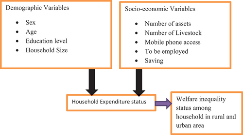
The conceptual Framework of this study indicate that through an analysis of the association among diverse socio-economic and demographic factors and the status of household expenditures- is a key indicator of a household’s economic situation and is directly linked to welfare inequality, we can gain a more comprehensive grasp of the status of inequality in terms of welfare among household in the rural and urban areas in Ethiopia. By pinpointing the primary drivers of this inequality, policymakers and stakeholders can formulate precise interventions and strategies to tackle these disparities and strive towards establishing a more just living environment for all citizens of Ethiopia (Figure 1).

Figure 1. Conceptual framework.

Source: Own Computing, 2023.

3. Research methodology

3.1. Description of the study area

Ethiopia is a country located in the Horn of Africa. It is bordered by Eritrea to the north, Sudan to the west, South Sudan to the southwest, Kenya to the south, Somalia to the east, and Djibouti to the northeast. Ethiopia has a population of over 115 million people, making it the second-most populous country in Africa. It is a diverse nation with more than 80 ethnic groups, each with its own unique language and culture. Amharic is the official language, but there are also many regional languages spoken throughout the country. In terms of socioeconomic conditions, Ethiopia has a predominantly rural population. Agriculture is the backbone of the economy, with the majority of Ethiopians engaged in subsistence farming. However, there has been significant urbanization in recent years, with the growth of cities like Addis Ababa, the capital, and other regional centers. Urban areas offer more diverse economic opportunities, including manufacturing, services, and trade. Despite progress, Ethiopia still faces challenges in terms of poverty and inequality. The government has been implementing various development initiatives to address these issues, including efforts to improve infrastructure, education, healthcare, and access to clean water.

3.2. Types of data

The data type is quantitative and The Living Standards Measurement Study (LSMS). The LSMS is an extensive household survey research enterprise that is executed by the World Bank. This initiative aims to provide top-tier data on the socioeconomic conditions prevalent in developing countries. The LSMS data about Ethiopia from 6770 households have been obtained from the Ethiopia Socioeconomic Survey (ESS), which is a collaborative venture between the Central Statistics Agency (CSA) of Ethiopia and the World Bank. The ESS is an all-encompassing survey that collects detailed information on various facets of household welfare, such as consumption, income, education, health, labor, and assets. The present study endeavors to draw a comparison between the determinants of welfare inequalities in urban and rural Ethiopia, to gain a better understanding of their similarities and differences.

3.3. Method of data analysis

A decomposition analysis was undertaken by dividing the origins of the inequality in welfare between urban and rural areas. This shall involve the computation of the Atkinson index of inequality for the urban and rural areas, with consumption expenditure per adult equivalent as the measurement of welfare. Furthermore, inequality in welfare determinants was investigated through a series of regression models (Quantile Regression), wherein welfare levels were regressed against a series of explanatory variables.

3.4. Atkinson Index

The Atkinson index, introduced by esteemed British economist Anthony Barnes Atkinson in 1970, is a widely recognized measure of welfare inequality that serves as an alternative to the conventional Gini coefficient. The index takes into account the welfare of all citizens and recognizes that achieving an equitable distribution of resources entails prioritizing the well-being of the most disadvantaged over the average per capita income (Afonso & Do Rosário Cabrita, 2015). In essence, the index gives greater importance to the lower-income segments of society in its computation of the degree of inequality.

The Atkinson Index is a measure based on the concept of “equally distributed equivalent income,” which refers to the income per person that would generate the same level of overall societal welfare as the current distribution if it were distributed equally among all individuals. This concept was introduced by Atkinson in 1970. The index is represented by A(ε), where ε is a parameter that represents the degree to which individuals are concerned about inequality. Higher values of ε indicate a greater concern for inequality, while lower values signify less concern for disparities in welfare distribution.

The Atkinson Index can be calculated using the following mathematical formula:

$A\left(\epsilon \right)=1-\left[\left(\mathrm{\Sigma }\left(y_i{}^{\mathrm{\Lambda }}1-\epsilon \right)\right)/N{)}^{\mathrm{\Lambda }}1/\left(1-\epsilon \right)\right)\left]/\right[\mathrm{\Sigma }\left(y_i\right)/N]$

Here, A (ε) refers to the Atkinson Index, ε refers to the inequality aversion parameter, y_i refers to the welfare of individual i, and N refers to the total number of individuals in the population. The Atkinson Index has a range of 0 to 1, with 0 representing total equality (everyone has the same degree of welfare) and 1 representing utter inequality (only one individual has all the welfare). An increase in the Atkinson Index signifies a rise in inequality, while a decrease in the index indicates reduced inequality. One important feature of the Atkinson Index is its sensitivity to the chosen value of ε, which allows policymakers and economists to customize the analysis based on their specific concerns regarding income or welfare inequality. This flexibility makes the Atkinson Index a valuable tool for evaluating disparities in economic welfare across populations, thereby contributing to informed decisions on issues related to social equity and income redistribution.

3.4.1. Quantile regression model

The OLS regression method assumes that the effects of repressors do not vary along the conditional distribution of the dependent variable. For example, the effect of schooling on household welfare is assumed to be the same at the bottom as well as at the top of the welfare distribution. However, if these effects vary along the household welfare distribution, quantile regressions, which provide models for different percentiles of the welfare distribution, constitute a parsimonious way to describe the whole distribution.

In the ordinary least square (OLS) method in linear regression analysis to estimate the conditional mean of the consumption expenditure given a collection of explanatory variables. The average change in consumer expenditure resulting from a change in the relevant explanatory variable is represented by the estimated coefficients in the regression (Table 1).

Table 1. Description of variables and expected signs use in a quintile regression model

Variables	Types of variables	Description
Consumption	Continuous	The amount of expenditure by household
Sex of household head	Dummy	takes the value of 1 if the household head is male and 0 if female
Age of the household head	Continuous	A continuous variable equal to the age of the head of the household
Education level	Continuous	Year of schooling
Asset	Continuous	Number of assets what the household has
Household size	Continuous	number of household members
Health insurance	Categorical	takes value of 1 if the HH is has access to health insurance service and 0 if not
Number of livestock	Continuous	Refers to the total number of livestock owned by the household in TLU
Own Mobile phone	Dummy	It takes value of 1 if the HH has own mobile phone and 0 if not. It has positive effect on welfare inequality
Employment	Dummy	It takes value of 1 if the HH is employed the last 12 month and 0 if not
Saving	Dummy	takes value of 1 if the HH save money and 0 if not

While the Koenker and Bassett (1978) quantile regression model is used to evaluate poverty determinants at various places along the expenditure distribution. It benefits from permitting parameter variation between consumption expenditure distribution quantiles. The quantile estimator is more effective than linear regression when errors are not normally distributed, making it a robust method since the estimated coefficients of the quantile regression are less susceptible to outliers of the dependent variable than OLS (Buchinsky, 1998; Cameron & Trivedi, 2005). To produce more accurate and reliable estimates, the standard errors were computed using bootstrapped methodologies (Koenker & Hallock, 2001). Additionally, it enables researchers to pre-define any distribution positions by their particular study questions (Hao & Naiman, 2007). The quantile regression is as follows:

(1) $Q_{\tau }ln\left(\frac{y_i}{x_i}\right)=x_i{\beta }_{\tau }+{\epsilon }_{i,\tau }$(1)

Where $Q_{\tau }ln\left(\frac{y_i}{x_i}\right)$ is suggesting to estimate the Log of total expenditure per adult equivalent per year of i^th household model at τ – th quantile (Qτ) of the distribution of the dependent variable (Y) conditional on the value of X. Following Koenker, R. and Bassett, G., Jr [4], the income of an individual is in the τ – th quantile if his income is higher than the proportion τ of the reference group of individuals and lowers than the proportion (1) τ −τ β is the estimated parameter for each explanatory variable correspondingly. Other notations remain the same meaning as they are indicated in equation (1)(1) $Q_{\tau }ln\left(\frac{y_i}{x_i}\right)=x_i{\beta }_{\tau }+{\epsilon }_{i,\tau }$(1) .

Assuming that the r-th quintile of the error term conditional on the regressors is zero

$(Q_{\tau }(\frac{u_{i,\tau }}{x_i}=0$)) then the r th—conditional quantile of i y concerning i x can be written as:

(2) $Q_{\tau }\left(\frac{y_i}{x_i}\right)=x_i{\beta }_{\tau }$(2)

3.4.2. Lorentz curve

The Lorentz curve is an illustrative representation of the allocation of wealth or income among a given population. Its function is to depict inequality by graphing the accumulated portion of the populace, ranging from the most indigent to the most affluent, on the X-axis as opposed to their accumulated share of wealth or income on the Y-axis. In the event of absolute parity, the Lorentz curve would manifest as a 45-degree diagonal line, otherwise known as the line of equality. The further the curve diverges from this line, the greater the degree of inequality.

4. Result and discussion

4.1. Inequality in welfare and explanatory variables

Table 2 presents information about various variables and their respective mean values in both rural and urban regions. Notably, the mean household size in rural areas is significantly greater (7.789) than in urban areas (3.776). This may result in larger households encountering more formidable obstacles in fulfilling necessities and sharing finite resources amongst family members, thereby giving rise to welfare disparities. Furthermore, concerning consumption, urban households demonstrate a higher average consumption (61513.67) compared to rural households (48140.17). This suggests that urban households possess superior access to goods and services, which in turn contributes to an elevated standard of living and greater welfare inequality as compared to rural households. Additionally, urban areas exhibit a higher average education level (14.797) in contrast to rural areas (13.467). A higher education level typically leads to better job prospects and increased income, implying that urban residents have greater access to quality education and contribute to welfare disparities.

Table 2. Summary of explanatory variables

	Rural				Urban
Variable	Mean (%)	Std. Dev.	Min	Max	Mean (%)	Std. Dev.	Min	Max
Household size	4.789	2.288	1	19	3.776	2.179	1	16
Age	44.63339	15.443	17	97	40.32285	14.68674	13	99
Total consumption	48140.17	45344.79	440	944110.8	72733.01	61513.67	2077.20	1143184
Education level	13.467	21.150	0	99	18.29114	14.79708	1	99
Number of Livestock	1.516	1.0040	1	8	2.289855	1.963651	1	15
Number of Assets	1.980077	0.139758	1	5	1.943639	0.230649	1	5
Sex (Male)	74.74				63.72
Mobile phone access(yes)	33.69				80.12
Health insurance (yes)	23.01				21.75
Employment for the last 12 months (yes)	1.35				6.17
Saving (yes)	22.43				55.49

The study finds that urban households exhibit a notably higher percentage number of mobile phones owner (80.12%) in comparison to rural households (33.69%). This trend may suggest that urban households have comparatively superior access to communication and information, which could potentially enhance their overall welfare through accessing information to make the right decision. Conversely, rural households demonstrate a considerably higher average health insurance access (23.01%) in contrast to urban households (21.75%). This indicates that rural residents have more advantageous access to health insurance, leading to better health outcomes and contributing to inequality in welfare. Furthermore, urban households present a marginally higher employment rate (6.17%) than rural households (1.35%). This may be attributed to the nature of employment opportunities in rural areas (such as agricultural and informal sector jobs) as opposed to the urban employment landscape (which mainly involves formal sector jobs). However, the difference is relatively small, suggesting that employment alone may not be a significant driver of welfare inequality.

The study also reveals that the mean number of assets is almost identical in rural (1.980) and urban households (1.943). This indicates that asset ownership may not be a significant factor in welfare inequality between rural and urban areas. A higher percentage of urban households make savings (55.49%) than rural households (22.43). This could imply that urban households are more prudent with their financial resources, which might eventually contribute to better welfare outcomes.

4.2. Inequality in welfare between Ethiopia’s urban and rural area

The estimation of welfare inequality is accomplished using the Atkinson index, which integrates individual income estimates with a parameter known as epsilon- in the Atkinson index reflects the degree of inequality aversion, or how much weight is given to the lower end of the income distribution. The higher the epsilon, the more sensitive the index is to changes in the incomes of the poor. The lower the epsilon, the more equal the index treats all incomes. Therefore, choosing an appropriate value for epsilon depends on the normative judgement of the analyst or the policy maker, intended to account for society’s inequality aversion. In this particular instance, the epsilon parameter has been assigned a value of 0.5- possible justification for assuming epsilon = 0.5 is that it represents a moderate level of inequality aversion, which may be suitable for a broad range of policy contexts. The index furnishes both group-specific and population outcomes, thus providing an overall suggestion of welfare inequality (Afonso & Do Rosário Cabrita, 2015). The results reflect the geographical location of welfare inequality, in both rural and urban settings. The Atkinson index, which is a measure of welfare inequality, estimates two distinct groups, one in a rural and the other in an urban area. Subsequently, these estimates are combined to produce a population estimate. The Atkinson index ranges from 0 to 1, with higher values indicating greater welfare inequality.

4.2.1. Result of Atkinson Index

Based on the results obtained, it can be deduced that the Atkinson index for the rural group is 0.123006, while it is 0.110899 for the urban group. These values suggest that rural areas exhibit a higher degree of welfare inequality when compared to their urban counterparts. The confidence intervals for both groups have also been reported, indicating that there is a 95% probability that the true Atkinson index value for rural areas lies between 0.111667 and 0.134345, while for urban areas, it falls between 0.102543 and 0.119254. Furthermore, the population Atkinson index has been provided, which stands at 0.124907. This value falls between the rural and urban indices, which is expected, given that it considers both groups. The confidence interval for the population index ranges from 0.118083 to 0.131731 (Table 3) (Figure 2).

Figure 2. Lorentz Curve.

Source: Own Computing result from LSMS, 2023.

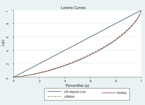
Table 3. Atkinson index for inequality in welfare among households in urban and rural areas

Index: Atkinson index
Parameter epsilon: 0.5
Group	Estimate	STE	LB	UB
1: RURAL	0.123006	0.005784	0.111667	0.134345
2: URBAN	0.110899	0.004262	0.102543	0.119254
Population	0.124907	0.003481	0.118083	0.131731

Source: own Computing Result from LSMS, 2023.

A study conducted by Aaberge and Brandolini in 2015 examined the correlation between economic deprivation and welfare inequality across several wealthy nations. Their findings revealed that welfare inequalities persisted across various geographic regions, with urban centers typically displaying a lower Atkinson index than rural areas. These results are consistent with the present study, which suggests that there is a greater degree of welfare inequality in rural areas as opposed to urban areas. Korzeniewicz and Moran (2009) posited that welfare inequality is particularly rampant in developing countries and regions characterized by poverty, low levels of education, and limited access to resources. The data obtained in this study lends support to this notion, indicating that rural areas, which are often underdeveloped and have inadequate access to resources relative to urban areas, may experience higher levels of welfare inequality.

4.2.2. Lorentz curve

The Lorentz curve is a graphical representation of the distribution of income or of wealth. It was developed by the American economist Max Lorentz in 1905. Here’s a breakdown of how it is constructed. The horizontal axis of the graph represents the cumulative percentage of the population (from poorest to richest), which is uniformly distributed ranging from 0 to 100%. The vertical axis represents the cumulative percentage of total income earned (or wealth owned), also ranging from 0 to 100%. A perfectly equal income distribution would be represented by a 45-degree diagonal line from the origin to the right-upper corner, known as the line of equality. For each point on the graph, its horizontal coordinate indicates what percentage of people own less wealth than this point, and its vertical coordinate indicates what percentage of total wealth they own. To construct the curve, we plot the proportion of the total income earned by the bottom 100% of the population against the value of income. This curve starts at the origin and ends at 100%, 100%. The curve lies below the line of equality, and the area between the curve and the line of equality represents the degree of income inequality in the population. In a nutshell, the more curved the Lorentz Curve (in other words, the larger the gap between the curve and the straight line), the higher the inequality. If the curve was a straight diagonal line, it would indicate perfect equality.

The result indicates that the Lorentz curve for urban households is situated above the Lorentz curve of rural households. This observation implies that the urban populace encounters a reduced degree of welfare inequality in comparison to their rural counterparts. In essence, welfare, be it consumption, is more uniformly distributed among urban households as opposed to their rural counterparts (Figure 2).

4.2.3. Comparison of consumption among household

Table 4 below present’s information on the proportions of urban and rural populations, mean income levels, relative mean income, income share, and log (mean) income for both urban and rural areas.

Table 4. Comparison of consumption among household in rural and urban area

Rural/Urban	Popn. share	Mean	Relative mean	Income share	log(mean)
Urban	0.53988	72733.01	1.18424	0.63935	11.19455
Rural	0.46012	48140.17	0.78382	0.36065	10.78187

Source: Own Computing result from LSMS, 2023.

In terms of population distribution, it can be observed that urban areas comprise 53.988% of the population, while the remaining 46.012% reside in rural areas. Thus, it can be inferred that urban areas have a marginally higher population density than rural regions. The mean consumption for urban and rural areas is 72,733.01 and 48,140.12, respectively. This indicates that, on average, individuals residing in urban areas consume more than those living in rural areas. The relative mean income for urban and rural areas is 1.18424 and 0.78382, respectively. This metric compares the average consumption between the two areas. A value greater than one denotes a higher mean income, while a value less than one indicates a lower income. In this case, urban areas have an income that is 18.424% more than that in rural areas.

The consumption share for urban and rural areas is 63.935% and 36.065%, respectively. This implies that urban areas have a larger proportion of total consumption than rural areas. This could be attributed to various factors such as better job opportunities and higher wages in cities.

The natural logarithm of mean income for urban and rural areas is 11.19455 and 10.78187, respectively. It is common practice to use logarithms to normalize data and reduce the impact of extreme values or skewness. The higher log (mean) value for urban areas confirms that urban areas have higher average consumptions as compared to rural areas. In conclusion, the results indicate a significant disparity between urban and rural areas concerning population distribution, mean income, and income share. Urban areas exhibit higher average income, greater population share, and a larger portion of total income than rural areas. Policymakers and analysts could leverage this information to derive insights regarding economic development, consumption distribution, and regional wealth disparities.

4.3. Determinates of inequality in welfare among household in urban and rural area

The study of the determinants of welfare inequality of households in rural and urban areas entails an in-depth exploration of the factors that give rise to inequality in living conditions between these two regions. To this end, the study used quantile regression, which takes into account both urban and rural areas, to explain the diverse impacts of these determinants across welfare distribution.

4.3.1. Determinates of inequality in welfare among urban households

The regression output in Table 5 illustrates the correlation between total consumption and a variety of independent variables for households situated in urban areas. Here we used quantile regression, which is a type of statistical analysis used in research and data analysis. It is particularly useful in situations where the relationship between variables may change across different levels of an outcome. Instead of just looking at the mean, quartile regression allows examining the relationship across multiple points in the distribution of a response variable, to identify the key determinates of welfare inequality among urban households. The result indicates that 0.25 quantile regression signifies that the coefficients denote the impact on the 25th percentile of the total consumption distribution for each variable. The findings of the regression output suggest that the level of education and the number of livestock are noteworthy determinants of inequality in welfare among urban households at the 25th percentile of total consumption. Conversely, variables such as household size, mobile phone ownership, access to health services, saving, and working in trade, appear to have little impact on welfare inequality.

Table 5. Empirical result for determinates of welfare inequality among households in rural and urban

	RURAL				URBAN
	OLS	25^th quantiles	50^th quantiles	75 quantiles	OLS	25^th quantiles	50^th quantile	75 quantiles
Age Square	1.365 (11.018)	5.273 (2.767)	5.238 (10.335)	−1.209 (16.524)	1.123 (4.883)	−0.463 (3.714)	−5.111 (5.834)	10.50373 (12.768)
Sex	−108079 (79733.63)	0	0	0	20064.13 (17860.04)	0	0	0
Household size	−6518.01 (5829.65)	−1497.51 (2012.233)	2786.094 (6845.37)	3339.066 (7961.523)	3433.209 (2217.985)	1768.888 (1362.825)	3258.708 (2007.275)	11244.55** (4850.884)
Education level	1087.60 (670.637)	221.148 (232.7081)	177.6208 (791.644)	186.163 (920.724)	−168.452 (165.398)	−226.948** (99.992)	−222.499 (147.275)	105.9487 (355.913)
Number of livestock	−43782.8 (15435.16)	−7278.55 (5454.817)	−11884.8 (18556.62)	−13768 (21582.31)	4591.672 (5486.229)	9834.755*** (3503.061)	8567.562 (5159.58)	−2715.9 (12468.91)
Own mobile phone	−43918.1 (36764.64)	4592.965 (12606.92)	−8096.15 (42887.18)	−13577.1 (49880.03)	−2352.01 (9251.727)	−1828.05 (5830.262)	1836.956 (8587.264)	14331.66 (20752.43)
Access to health insurance	10338.33 (12100.03)	38221.16*** (12773.19)	36205.24 (43452.81)	41797.55 (50537.89)	2155.348 (4200.897)	1518.823 (8089.293)	−6640.82 (11927.8)	−46307.5 (28825.33)
Employment	0	0	0	0	0	0	0	0
Number of Assets	0	14766*** (4597.784)	21056.8*** (7555.824)	47744*** (15256.78)	0	2294 (14924.43)	17849.72 (18323.5)	−26631.2 (290784.9)
Saving	317577.7 (30478.66)	18849.69* (10771.47)	18580.87 (36643.23)	3127.464 (42617.99)	2406.371 (9681.786)	9551.557 (6302.655)	16020.06* (9283.04)	986.0932 (22433.88)
_cons	387863.8 (138100.5)	22497.63 (28132.27)	41603.18 (95702.54)	83805.29 (111307.1)	−307.254 (39911.1)	−3667.03 (37579.3)	−50832.6 (55349.72)	−56106.5 (133761)
Pseudo R^2	0.287	0.277	0.331	0.237	0.182	0.133	0.113	0.151

*** Significance at one % significance level, ** significance at 5% significance level, * significance at 10% significance level.

Source: Own Computing result from LSMS, 2023.

The quantile regression analysis reveals that education level has a significant negative relationship with total consumption at the 25th percentile, with a coefficient of −226.948 and a standard error of 99.99156. The t-value of −2.27 and p-value of 0.027 further support this finding. This suggests that higher education levels are associated with lower total consumption and could exacerbate welfare inequality in urban areas. Furthermore, the number of livestock has a significant positive relationship with total consumption, with a coefficient indicating that an increase of one unit in TLU leads to an annual increase of 9834.75 units in total consumption. This finding indicates that owning more livestock is linked to higher total consumption, further contributing to inequality in welfare among urban households in urban areas. Policymakers may use this to support livestock-rearing initiatives, given its influence on total consumption and economic welfare.

Table 5 presents the outcomes of a quantile regression analysis with a 0.5 quantile, which examines the correlation between the determinants of welfare inequality and total consumption, particularly among urban households. The model takes into account various factors, such as household size, educational attainment, number of livestock, ownership of a mobile phone, and access to health services, wage jobs, employment, savings, and work in trade. On the other hand, the coefficients of saving are significant at a 0.09 level, indicating that there exists some indication of a link between these determinants and welfare inequality in urban areas. For savings, the coefficient is positive (16020.06), denoting that households with greater savings tend to exhibit higher levels of total consumption. Nevertheless, it is noteworthy that these associations are not highly significant.

The utilization of the 0.75 quantile regression output for the urban area was employed to examine and realize the determinants of inequity in welfare. Multiple factors were assessed, encompassing household size, education level, number of livestock possessed, possession of mobile phones, accessibility to health amenities, employment status, savings, and involvement in trading activities (Table 5). It was established that household size exhibited a substantial positive influence on welfare inequality, with a coefficient of 11,244.55. This denotes that when the household size is augmented by one unit, the overall consumption of the household escalates by 11,244.55 units annually, as does welfare inequality at this quantile. This correlation between household size and welfare inequality has been noted in alternative research.

4.3.2. Determinates of inequality in welfare among rural households

The outcomes illustrated in Table 5 reveal that a quantile regression analysis at the 0.25 percentile level, was conducted to identify the determinants of inequality in welfare among rural areas. The coefficients presented to signify the partial effects that the independent variables exert on the total consumption at the 0.25 percentile. In simpler terms, they uncover the relationship between the 25th percentile of total consumption and the impact of a one-unit increase in each independent variable, while keeping other factors constant. The evidence suggests that the availability of health services has a positive and statistically significant influence on total consumption. This implies that the accessibility of health services is a crucial driver of welfare in rural areas, which aligns with the conclusions of Case and Deaton’s (2005) study highlighting the affirmative relationship between health service availability and welfare in rural India. Furthermore, the possession of assets has a positive and statistically significant impact on total consumption, indicating that households with more assets have higher levels of welfare. This observation corresponds with the findings of Sahn and Stifel (2003), who explored the connection between asset ownership and welfare in rural Mozambique. Saving also has a positive and marginally significant effect on total consumption, implying that households with higher savings could have higher welfare levels, although this effect is not statistically significant at the 95% confidence level.

This result supports Ethiopian policies that aim to increase access to health services for rural populations, promote asset accumulation, and encourage saving. In terms of assets, Ethiopia has been implementing various agricultural and rural development programs, such as the Sustainable Land Management Program, the Productive Safety Net Program, and the Rural Financial Intermediation Program. These policies aim to increase the agricultural productivity and income of rural households, which could enable them to accumulate productive assets and increase their consumption and welfare. For savings, Ethiopia has been promoting micro-saving schemes and rural saving and credit cooperatives to enhance the financial inclusion and saving capacity of rural households.

Table 5 presented a 0.5 quantile regression analysis for the determinants of inequality in welfare in a rural household. From the findings, it is evident that the number of assets owned by a household has a large and significant positive impact on welfare inequality, as evidenced by the coefficient of 21,056.8 and p-value of 0.006 (p < 0.05). This suggests that a unit increase in the number of assets held by a household leads to a substantial rise in welfare inequality. This is consistent with previous literature highlighting the role of assets in determining household welfare and inequalities (e.g., Günther & Klasen, 2009).

The findings from Table 5 present a 0.75 quantile regression analysis that centers on elucidating the interconnection between multiple factors and their determinants on the issue of inequality in welfare in rural localities. The outcomes reveal that the variable of Asset Quantity holds a statistically significant positive influence on overall consumption in rural regions, with a coefficient of 47,744 and a p-value of 0.002. This suggests that households with a greater number of assets tend to demonstrate a higher level of welfare, as evidenced by their higher total consumption. However, the OLS result indicates that any of the explanatory variables have no statistically significant effect on inequality in welfare among households in rural and urban.

5. Conclusion and policy implication

The study has examined the welfare inequality among rural and urban households in Ethiopia, using the Atkinson index and quantile regression methods. The study has found that there is a significant difference in welfare inequality between rural and urban areas, with rural areas having a higher degree of inequality. The study has also identified the main factors that determine welfare inequality in different consumption percentiles for both rural and urban households. The study has implications for policy and practice to reduce welfare inequality and improve the well-being of the population. The study suggests that education level and livestock production are important determinants of welfare inequality among urban households in the lower consumption percentiles, while household size is the only significant factor in the higher consumption percentiles. Therefore, policies aimed at reducing welfare inequality in urban areas should focus on enhancing educational opportunities and promoting livestock activities, especially for the poor and vulnerable groups. Moreover, policies should also consider the effects of household size on welfare inequality and explore ways to support larger households.

The study also indicates that asset accumulation, saving and health access are key determinants of welfare inequality among rural households in both lower and higher consumption percentiles. Hence, policies aimed at reducing welfare inequality in rural areas should emphasize the promotion of asset ownership, saving behavior and health service provision, which can improve the living standards and resilience of rural households. Furthermore, policies should also investigate the other factors that may influence welfare inequality in rural areas, such as mobile phone ownership, trade and education.

5.1. Limitation of the study

The study on the Determinants of Inequalities in Welfare among Households in Ethiopia, focusing on the urban and rural divide, possesses several limitations that warrant consideration. Firstly, the research may face challenges in generalizing its findings to the entire Ethiopian population, as the scope is confined to urban and rural areas, potentially overlooking nuances in peri-urban or other specific contexts. Additionally, the accuracy and reliability of the results may be influenced by the quality of data, potentially affected by recall biases or data collection limitations. Moreover, the study might not adequately address cultural and contextual variations within urban and rural settings, limiting the depth of its analysis. Finally, external factors such as political and economic changes that occurred after the study period could impact the relevance and applicability of the findings to the current socio-economic landscape in Ethiopia.

Abbreviation

LSMS: Living Standards Measurement Surveys; SDGs: Sustainable Development Goals; GTP: Growth and Transformation Plan; HDI: Human Development Index

Author contribution

All Authors have written and analyzed all parts of the paper together

Availability of data and materials

The data can be obtained from the corresponding author upon request

Disclosure statement

No potential conflict of interest was reported by the author(s).

Additional information

Funding

The authors have not received funding for this research.

Notes on contributors

Tsegamariam Dula

Tsegamariam Dula is an accomplished academic and researcher, currently serving as a lecturer and researcher at Wolkite University in Ethiopia. He is A development Studies Specialist. He is also a PhD Candidate in development studies at Addis Abeba University. His research interests are wide-ranging, but he has a particular focus on issues related to development studies, livelihood security, Inequality, food security, agricultural economics, natural resource management, agricultural extension, and climate-smart agriculture.

Jemil Yasin

Jemil Yasin is a Development Studies Specialist and PhD Candidate at Addis Abeba University. His research interests are food security, Poverty reduction, and agricultural extension.

Haymanot Meseret

Haymanot Meseret is a Ph.D. candidate at the Center for Rural Development Studies, Addis Ababa University.

Abrham Seyoum

Abraham Seyoum (Ph.D.) is an Associate Professor at the Center for Rural Development Studies, Addis Ababa University.

References

- Afonso, H., & Do Rosário Cabrita, M. (2015). Developing a lean supply chain performance framework in an SME: A perspective based on the balanced scorecard. Procedia Engineering, 131, 270–17. https://doi.org/10.1016/j.proeng.2015.12.389
- African Development Bank (AfDB). (2012, March). Briefing note 5: Income inequality in Africa.
- Alemu, T. (2011). Rural welfare and agricultural Development in Ethiopia: Challenges and prospects. International Journal of Economics and Finance, 3(5), 132–142.
- Alemu, T., Alemayehu, W. A., & Bedane, G. (2018). Determinants of income inequality in Eastern Zone of Tigray region: A simulation of decomposition analysis. African Journal of Economic Review, 6(1), 01–17.
- Ali, L. R., Ramay, M. I., & Nas, Z. (2013). Analysis of the determinants of income and income gap between urban and rural Pakistan. Interdisciplinary Journal of Contemporary Research in Business, 5(1), 858–885.
- Anyanwu, J. C. (2005). Rural poverty in Nigeria: Profile, determinants and exit paths. African Development Review, 17(3), 435–460. https://doi.org/10.1111/j.1017-6772.2006.00123.x
- Assefa, A., & Letamo, G. (2019). Determinants of access to education in Ethiopia. Journal of African Development, 21(2), 27–42.
- Beyene, A. D., & Mekonnen, A. (2014). Determinants of public and private sector demand for education in Ethiopia. International Journal of Education Economics and Development, 5(2), 163–180.
- Buchinsky, M. (1998). Recent advances in quantile regression models: A practical guideline for empirical research. The Journal of Human Resources, 33(1), 88–126. https://doi.org/10.2307/146316
- Cameron, A. C., & Trivedi, P. K. (2005). Microeconometrics: Methods and applications. Cambridge University Press.
- Case, A., & Deaton, A. S. (2005). Broken down by work and sex: How our health declines. In Analyses in the economics of aging (pp. 185–212). University of Chicago Press.
- Central Statistical Agency (CSA) & ICF. (2016). Ethiopia demographic and health survey 2016. CSA and ICF.
- Central Statistical Agency of Ethiopia. (2016). Ethiopia: National accounts statistics. CSA.
- Chamarbagwala, R. (2010). Economic liberalization and urban–rural inequality in India: A quantile regression analysis. Empirical Economics, 39(2), 371–394. https://doi.org/10.1007/s00181-009-0308-4
- Chameni Nembua, C., & Miamo Wendji, C. (2012). Inequality of Cameroonian households: An analysis based on shapley-shorrocks decomposition. International Journal of Economics and Finance, 4(6), 149–156. https://doi.org/10.5539/ijef.v4n6p149
- Dercon, S., & Krishnan, P. (2000). Vulnerability, seasonality and poverty in Ethiopia. The Journal of Development Studies, 36(6), 25–53. https://doi.org/10.1080/00220380008422653
- Dorosh, P., & Schmidt, E. (2010). The rural-urban transformation in Ethiopia. Ethiopian Development Research Institute, Working Paper 13.
- Gebeyehu, B., Feleke, S., Tufa, A., Lemma, T., Tewodros, T., & Manyong, V. (2018). Patterns and structure of household income inequality in rural Ethiopia. World Development Perspectives, 10-12, 80–82. https://doi.org/10.1016/j.wdp.2018.09.007
- Girma, W., & Genebo, T. (2014). Determinants of nutritional status of women and children in Ethiopia. ORC Macro.
- Günther, I., & Klasen, S. (2009). Measuring chronic non-income poverty. Poverty Dynamics: Interdisciplinary Perspectives, 16, 77.
- Hao, L., & Naiman, D. Q. (2007). Quantile regression. Sage Publications.
- Koenker, R., & Bassett, J. G. (1978). Regression quantiles. Econometrica Journal of the Econometric Society, 46(1), 33–50. https://doi.org/10.2307/1913643
- Koenker, R., & Hallock, K. (2001). Quantile regression. Journal of Economic Perspectives, 15(4), 143–156. https://doi.org/10.1257/jep.15.4.143
- Korzeniewicz, R. P., & Moran, T. P. (2018). Unveiling inequality: A World-historical perspective. Routledge.
- Kuznar, L. A. (2019). Ethiopian inequality report. Research, innovation excellence report.
- Mossie, T. B., & Demissie, S. F. (2020). Factors affecting inequality in living standards in Ethiopian cities: The case of the town of Bedele. Public Administration and Economic Affairs, 1(1), 33–42.
- Muleta, E. A., & Belete, T. H. (2017). Transformation cooperation on urban and regional development in Ethiopia: The example of the sustainable urban development project. In M. Massa (Ed.), Partnership for change shaping transformation in Ethiopia. Friedrich-Ebert-Stiftung.
- Ravallion, M., & Wodon, Q. (2000). Does poorer mean less happy? Subjective well-being and income dynamics in rural Ethiopia. 210(2), World Bank Publication
- Sahn, D. E., & Stifel, D. (2003). Exploring alternative measures of welfare in the absence of expenditure data. Review of Income and Wealth, 49(4), 463–489. https://doi.org/10.1111/j.0034-6586.2003.00100.x
- Teshome, G., Sera, L., & Dachito, A. (2021). Determinants of income inequality among urban households in Ethiopia: A case of Nekemte Town. SN Business & Economics, 1(11), 1–21. https://doi.org/10.1007/s43546-021-00158-2
- UNDP. (2015). Human development report 2015: Work for human development. UND
- United Nations. (2015). Transforming our world: The 2030 agenda for Sustainable Development. United Nations.
- United Nations Development Programme (UNDP). (2014).
- Woldehanna, T., Hagos, A., & Haile-Gebriel, Z. (2005). The impact of policy changes on consumption, education, saving, and poverty in Ethiopia. Chronic Poverty Research Centre (CPRC) Working Paper 37.
- World Bank. (2015). Ethiopia poverty assessment. World Bank.
- World Bank. (2016). Poverty and shared prosperity 2016: Taking on inequality. World Bank.
- World Bank. (2017). Ethiopia – poverty assessment. World Bank Group.
- World Bank, W. (2014). Ethiopia poverty assessment. World Bank.