Data analysis and interpretable machine learning for HVAC predictive control: A case-study based implementation

Abstract

Energy efficiency and thermal comfort levels are key attributes to be considered in the design and implementation of a Heating, Ventilation and Air Conditioning (HVAC) system. With the increased availability of Internet of Things (IoT) devices, it is now possible to continuously monitor multiple variables that influence a user’s thermal comfort and the system’s energy efficiency, thus acting preemptively to optimize these factors. To this end, this paper reports on a case study with a two-fold aim; first, to analyze the performance of a conventional HVAC system through data analytics; secondly, to explore the use of interpretable machine learning techniques for HVAC predictive control. A new Interpretable Machine Learning (IML) algorithm called Permutation Feature-based Frequency Response Analysis (PF-FRA) is also proposed. Results demonstrate that the proposed model can generate accurate forecasts of Room Temperature (RT) levels by taking into account historical RT information, as well as additional environmental and time-series features. Our proposed model achieves 0.4017 °C and 0.9417 °C of Mean Absolute Error (MAE) for 1-h and 8-h ahead RT prediction, respectively. Tools such as surrogate models and Shapley graphs are employed to interpret the model’s global and local behaviors with the aim of increasing trust in the model.

Introduction

Background

Research has shown that thermal comfort levels in the workplace have a significant impact on the productivity of workers (Seppanen, Fisk, and Lei 2006). The running costs of a Heating, Ventilation and Air Conditioning (HVAC) system to maintain a productive temperature is ten times lower compared to the economic losses incurred because of lower worker productivity in a free-running building (McCartney and Humphreys 2002). On the other hand, energy usage in buildings has witnessed a continuous and increasing trend of more than 10EJ in the past decade, according to the International Energy Agency (IEA) (IEA 2021). This gives rise to challenges such as energy shortage and global warming, which have become more imminent worldwide. The energy efficiency of HVAC systems is thus a topical issue that requires attention and methods for managing effectively. This work discusses the use of interpretable machine learning techniques for developing a predictive control strategy. The machine learning nature of the proposed technique aspires to the realization of an autonomous HVAC system while the interpretable nature is aimed at making the strategy trusted and reliable.

Research gaps

A wealth of research has been carried out to optimize an HVAC system’s energy efficiency while maintaining thermal comfort levels. In many of these research studies, predictive model control is used to adaptively tune the HVAC system to achieve such optimization. In the work by Kelly and Bushby (2012) and Li et al. (2015), the energy-saving performance of traditional control methods is compared to that of machine learning-based approaches for an HVAC system installed in a real building. They determined that using intelligent agents to manage the HVAC system has promising performance in terms of energy efficiency optimization. As a specific example, the experimental results from the research (Li et al. 2015) reported an average of 20% energy saving with a concurrent improvement in thermal comfort in the tested area.

Some studies, however, report on the limitations of employing Machine Learning (ML) methods for optimizing building energy efficiency. Miller et al. (2022) investigated the model performance from more than 4000 competitors in the Great Energy Predictor III challenge (Miller et al. 2020) and concluded that the prediction errors in the test phase are mainly caused by the fact that these models are unable to predict behavior which did not appear in the training phase. Furthermore, the absence of model interpretability prevents such models from being adopted for HVAC system management. This is due to the fact that a model could potentially learn spurious association relationships, which would be difficult to unmask without proper insights into the model’s underlying mechanisms. While introducing a higher number of features typically boosts the model’s prediction accuracy, there is a risk that some irrelevant features could cause the model to learn from spurious non-causal knowledge (Little and Badawy 2019). A black-box model that lacks interpretability can lead to business and ethical concerns. For example, business owners often cannot bear the economic and security risks of applying unknown black-box models to critical areas of HVAC systems management (Chew and Yan 2022). In the study by Mao and Grammenos (2021), the importance of the interpretability of machine learning models used in the design of HVAC systems is discussed. The authors argue that interpretable models can unveil potential optimization strategies and determine the reasons that lead to incorrect predictions.

Main contributions

The work reported in this paper acts as a stepping stone toward the vision of eventually realizing a trusted and autonomous HVAC system. To achieve autonomy, there is a two-fold requirement: first, the control strategy needs to self-configure and self-adapt itself to respond to users’ needs without intervention from the users themselves; secondly, the strategy should control the HVAC unit to operate with a balanced tradeoff between thermal comfort and energy efficiency. To achieve trust, the model should have a certain level of interpretability allowing the machine-made decisions to be understandable by humans.

To this end, the main contributions of this work¹

may be summarized as follows:

• The exploratory data analysis carried out on a building dataset in previous work is extended by performing additional stationarity analysis on the given dataset. This extended analysis motivated our decision to include historical room temperature (RT) information in our machine-learning model.

• We propose and implement a machine learning model employing an extreme gradient boosted machine (XGBM) which together with enhanced feature engineering achieves 0.4017 °C and 0.9417 °C of Mean Absolute Error (MAE) for 1-hour and 8-hour ahead room temperature (RT) prediction in real-time. It is envisioned that such a model could be incorporated into a system that would allow autonomous operation of an HVAC unit.

• Using global and local Interpretable Machine Learning (IML) techniques, we explain the working mechanisms of the proposed XGBM-based HVAC predictive control model that was implemented, which in turn contributes to increased trust of the model by human users and operators.

• Beyond the commonly used IML techniques, we propose a new Permutation Feature-based Frequency Response Analysis (PF-FRA) technique to enhance the model’s global interpretability. The proposed PF-FRA technique quantifies the contribution of each feature in the frequency domain, compared to existing IML techniques which, to the best of the authors’ knowledge, can only explain ML models in the time domain. This frequency domain approach allows us to understand which features contribute to the high-frequency and Direct Current (DC) components of the model response, which in turn reflect fluctuations and key magnitude components, respectively.

Paper structure

The remainder of this paper is organized as follows: Section “Related work” reviews related research work across two domains; the first domain looks at ML techniques for optimizing thermal comfort and energy efficiency; the second domain looks at techniques for predicting temperature in non-domestic buildings. Section “Methodology” presents our methodology for carrying out this work from the data acquisition and processing stages through to the model’s selection, evaluation and interpretation. Section “Data analysis: results and discussion” reviews key results from the exploratory data analysis carried out in previous work and extends it through additional stationarity analysis. This latter analysis in turn is used to inform the enhanced feature engineering that was adopted and which led to a boost in predictive model performance. Section “Predictive modeling: results and discussion” presents and discusses the results obtained from the evaluation of the XGBM-based model that was developed, as well as its behavior through interpretability analysis. Finally, Section “Conclusion” concludes this paper and provides suggestions for future research work.

Related work

This section reviews the literature across two broad domains: The first domain, summarizes recent studies that aim to optimize an HVAC system’s thermal comfort and energy efficiency performance using predictive control or machine learning-based methods. The second domain investigates machine learning techniques used for indoor temperature prediction.

Thermal comfort and energy efficiency optimization

Scholars have proposed advanced machine learning models with the goal of achieving optimal energy efficiency and thermal comfort levels. For example, Satrio et al. (2019) proposed a hybrid method employing an Artificial Neural Network (ANN) and a multi-objective genetic algorithm to generate a control strategy that would enable HVAC systems to be operated efficiently. In a similar manner, Ahn and Park (2020) utilized a deep Q-network (DQN) to realize optimal control balancing between multiple HVAC systems, reducing the total energy consumed by the HVAC systems under consideration by more than 15.7% compared to the baseline.

To maintain appropriate indoor thermal comfort levels, researchers in (Qin and Wang 2022) proposed a multi-discipline control method to predict the optimal environmental parameter values using a support vector machine (SVM) and to control the indoor temperature using a reinforcement learning method. In the work by Xu et al. (2018), a feedback-data-based learning approach is proposed to quantify thermal comfort in a complaint-driven environment control system, achieving a satisfactory Set-Point Temperature (STP) level for all occupants.

Indoor temperature prediction

In terms of indoor temperature prediction, many recent studies have focussed on using machine learning techniques, both traditional statistical learning and more topical deep learning techniques, to generate robust and accurate prediction models.

Conventional machine learning models have proved to be quite successful in predicting indoor room temperature (RT) accurately. Paul et al. (2018) compared the indoor temperature prediction performance for three popular regression models: Random Forests (RF), Support Vector Machines (SVM) and Neural Networks (NN). Trained with an online learning strategy, these models generate their prediction based on a number of indoor and outdoor features with the readings captured by real sensors. It is found that the RF model has the lowest coefficient of variance at 0.0840 with the best R-squared score at 0.9855.

Arendt et al. (2018) investigated a variety of machine learning models with different levels of interpretability, categorized into the so-called white-box, grey-box and black-box models for a university building. Assuming a loss of model transparency, the most accurate black-box model in the option pool outperforms the best grey- and white-box models by 0.3 °C and 0.6 °C, respectively. However, the dataset used only covers a single month period, which provides limited reliability in terms of model robustness.

A more comprehensive study by Alawadi et al. (2022) compared 36 models from 20 different algorithm families, including Bayesian, ensembles, linear, Gaussian, and neural networks to name but a few. Similar experimental results from other researchers (Paul et al. 2018) indicate that tree-based regressors achieve better performance in terms of R-squared scores compared to NN-based models and SVMs. The authors of these studies state that the possible reason for this performance is that a tree-based model tends to be less noise-sensitive, and thus it is likely to have better robustness against outliers than the more complex models like NN.

Neural networks, however, are well-suited for approximating non-linear systems. In the study by Li, Ren, and Wang (2013), the authors argue that it is challenging to perform accurate control using conventional modeling methods due to the non-linear nature of an HVAC system. To this end, the authors propose a Back Propagation NN (BPNN) to predict the temperature of a room. Studies dating back to 2006 (Ruano et al. 2006) have also considered the use of simple neural networks to perform long-term indoor temperature prediction, however, multi-objective genetic algorithms are applied to optimize the model parameters instead of the gradient descent approach employed in (Li et al. 2013).

While in the aforementioned studies, the indoor temperature is treated as a categorical feature, there are studies that treat temperature as a time series feature. For example, Mateo et al. (2013) propose a hybrid model combining a Multilayer Perceptron (MLP) with a Non-linear Autoregressive Exogenous (NARX) network for indoor air temperature prediction. Evaluated using the Mean Absolute Error (MAE), its performance exceeds both traditional machine learning models and simple MLP models.

More advanced time series models make use of Recurrent Neural Networks (RNN). For example, in the study by Godahewa et al. (2020), an RNN is introduced to predict the temperature of a university’s lecture theater when it is occupied. It is shown that this RNN based approach outperforms other machine learning models like SVM, RF, MLP and Feed-Forward Neural Networks (FFNN) in terms of Root Mean Squared Error (RMSE). However, one of the recognized drawbacks of RNN is that it can only consider its previous outputs within a short term, and thus it tends to fail in predicting a time series that depends on relatively long historical patterns.

As a variant of RNN, the Long-Short-Term Memory (LSTM) model is designed to overcome RNN’s limitations. A recent study conducted by Xu et al. (2019) presents a novel modified LSTM model for 5-min and 30-min ahead indoor temperature prediction, which slightly improves the prediction performance compared to other traditional machine learning and NN-based models.

The aforementioned literature review is summarized in Table 1. It should be highlighted that the dataset period under consideration for all of these studies is quite limited ranging from one year down to merely a few minutes or seconds. Contrary, in our work presented in this paper, the dataset period spans almost three years, thereby allowing more room for validation across different seasons and years.

Table 1. Summary of key literature for indoor temperature prediction.

Modeling technique	Authors	Year	Dataset period	Sampling interval	Site	Main contributions	Limitations	Goal of the work
Traditional Machine Learning	Paul et al.	2018	1 month	15 min	Residential building	Trained with an online learning strategy, various traditional machine learning models to predict the indoor air temperature are compared. The selected model is furhter integrated into a IoT architecture for energy consumption prediction in a smart building.	Limited data is used for training and testing,and thus the model’s robustness needs further validations.	Formulate a ML-based mechanisumthat integrates the IoT and some widely used machine learning algorithms to create a predictive model that can be used for forecasting of smart building indoor temperature.
	Arendt et al.	2018	1 month	Not indentified	University Building	Investigate a variety of machine learning models with different levels of interpretability and find that the black-box model outperforms gray- and white-box models with smaller error.	Similar to the above.	Compare indoor temperature prediction performance between white-, gray- and black-box ML models in teaching buildings.
	Alawadi et al.	2020	9 months	10 min	University Building	Comprehensively compare 36 models from 20 different algorithm families, where the tree-based regressors show a better performance than NN-based models and SVM. It deduced that this might because tree- based models tend to be less noise-snesitive.	Fails to involve any features or indicators from the HVAC system.	Find the most suitable ML algorithm in terms of the performance and robustness that can be integrated into building management systems to improve building energy efficiency by comparison.
Neural Networks (NNs)	Ruano et al.	2006	21 d	5min	Seconday School Building	A simple NN is used to perform long-term indoor temperature prediction, while multi-objective genetic algorithms are applied to optimize the model parameters.	Simulations only cover a half month in winter. Does not consider the problem as a time series.	Apply multi-objective genetic algorithms to design a NN which aims to tune the indoor temperature for energy saving.
	Li et al.	2013	20 s	0.1 sec	Lab with HVAC System	A BPNN is designed to approximate the non-linear HVAC system with promising predicting capability with the respect to the energy efficiency.	Very limted data and covered period may imply overfitting for the NN. Does not consider the problem as a time series.	Use neural network-based method to approximate the non-linearity in HVAC systems to achieve accurate control.
	Mateo et al.	2013	1 year	1 h	Workshops, Functional Rooms	A hybrid model combining a MLP with a NARX is proposed,which outperforms other modelslike RMLR, ELM, ARX and MLP.Further introduce a clustering modelto group observations to boost prediciton accuracy.	Only performs short-term temperature prediction.	Validate the effectiveness of applying different ML techniques in predicting room temperature which is one of the most significant variables in energy management in buildings.
	Xu et al.	2019	2 months	5 min	Not identified	A novel modified LSTM model involving error correction mechanism is presented.for 5-min and 30-min ahead indoor temperature prediction.	Prediction is in short term and only the historical temperature is used as the single feature.	Predict indoor temperature by using modified LSTM model to provide a further reference to the feasibility study of indoor temperature prediction model.
	Godahewa et al.	2020	3 months	15 min	University Building	a RNN is introduced to predict the temperature of a university’s lecture theater. Simulations on the real data in this work further demonstrate that implementing the optimized RNN model in the HVAC controlling system contributes to around 20% more of energy saving.	A global temperature prediction model which can predict the future temperatures related to any room type is expected.	Explore how to optimize the setpoint temperature in an unoccupied room by applying time-series preidictive models.

It is also worth noting that despite witnessing significant improvements using increasingly more sophisticated black-box models such as SVMs and NNs, loss of interpretability and trust can lead to safety and ethical concerns. Therefore, one of the key considerations of our work presented in this paper is the use of interpretability techniques with the goal of explaining the underlying mechanisms of the models implemented with a view to improving trust and reliability.

Methodology

Figure 1 depicts the framework adopted in this work from the data acquisition phase through to the interpretation of the machine learning model employed. The process starts with the collection of data from different sensors including HVAC status indicators, as well as environmental data from indoor and outdoor sensors. After pre-processing the data and addressing challenges such as different sampling strategies and time misalignment, comprehensive Exploratory Data Analysis (EDA) is conducted to investigate the data distribution of the predictor and target variables, followed by stationarity and hidden pattern analysis. By recursively optimizing our feature engineering strategy based on knowledge discovery from the EDA process, we extract important information that is subsequently used in the predictive modeling phase.

Fig. 1. Framework of data acquisition, processing and modeling phases.

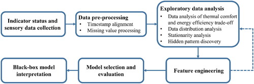
During the model selection and evaluation stage, we initially select and tune a number of candidate machine learning models, including both traditional and NN-based algorithms, by using training and validation sets. The best candidate model is then evaluated on the test set based on three commonly used metrics, including the Mean Squared Error (MSE), the Mean Absolute Error (MAE) and the R-squared score. Finally, an important aspect and contribution of our work is to interpret the machine learning model used from both local and global perspectives with the goal of unveiling the model’s inner working mechanisms. To this end, a new interpretability technique is proposed, which we call Permutation Feature-based Frequency Response Analysis (PF-FRA). This technique analyzes the response of the features in the frequency domain, complementing the conventional interpretability techniques which analyze the model in the time domain.

In the subsections that follow, we discuss the underlying theoretical principles and methods that are used in our data analysis and predictive modeling framework. It is worth noting that this work considers a specific case study of a commercial office building located in Athens, Greece.

Dataset description and pre-processing

The data considered in this work was acquired from both indoor and outdoor sensors and system indicators of an HVAC system installed in an 11-story commercial office building in Athens, Greece between December 2017 and September 2020. This reflects a time period of almost three years, which is markedly longer compared to the dataset periods considered in other studies discussed in Section “Related work”. The building did not employ any other sensors except the ones provided in the dataset. It is worth highlighting that this is not a new build and was constructed in the 1990s with some refurbishments in the HVAC system over the past decades. For this work, we considered Room 103 of the three rooms available in the dataset. Room 103 was located on the fifth floor of this building with a southwest orientation, thus facing toward the sun and calling for higher usage of air-conditioning. A summary of the pre-processed dataset characteristics is provided in Table 2.

Table 2. Summary of features in the pre-processed dataset.

Features		Number of observations	Sampling interval	Description	Min.	Max.	Mean	Probability (True)
Indoor features	HVAC On/Off state	137,116	10 min	A binary variable to indicate if the HVAC system is on, where 0, 1 represent Off, On.	N/A	N/A	N/A	0.2060
	HVAC operation mode	136,868	10min	A categorical variable to indicate the HVAC system’s operation mode, where 1, 2, 3 represent cooling, heating, ventilation.	1	3	N/A	N/A
	Room occupancy	136,868	10 min	A binary variable to indicate if the room is occupied, where 0, 1 represent unoccupied, occupied.	N/A	N/A	N/A	0.1447
	Historical room temperature	136,522	10 min	A continuous variable of room temperatures at 10 min ago.	14.0000	39.5000	25.2308	N/A
	Set point temperature	137,399	10 min	A continuous variable of set point temperature.	19.0000	28.0000	24.9897	N/A
Outdoor features	Outdoor air humidity	62,479	State-change basis	A continuous variable of outdoor air humidity.	37.9350	86.8150	60.6714	N/A
	Outdoor air temperature	27156	State-change basis	A continuous variable of ourdoor air temperature.	0.9000	37.2000	20.6545	N/A
Time series features	Season	136,416	N/A	A categorical variable to indicate the season where 1, 2, 3, 4 represent spring,summer, autumn and winter.	1	4	N/A	N/A
	Month	136,416	N/A	A categorical variable to indicate the month number.	1	12	N/A	N/A
	Day of Week	136,416	N/A	A categorical variable to indicate the day of week from Monday to Sunday.	0	6	N/A	N/A
	Hour	136,416	N/A	A categorical variable to indicate the hour in a day in 24-h format.	0	23	N/A	N/A
	Holiday	136,416	N/A	A binary variable to indicate if the date is a holiday.	N/A	N/A	N/A	0.308

As can be seen from Table 2, the dataset comprises indoor (I), outdoor (O) and time series (TS) features. For brevity, we shall refer to these as IOTS features. Two key challenges had to be addressed to convert the raw data acquired from the sensors into a structured dataset.

First, it can be observed that the sampling strategy differs amongst the IOTS features. Some features are sampled periodically on a 10-min basis while others are measured on a state-change basis. Secondly, time misalignment, typically caused by occasional sensor malfunction, causes a mismatch between the feature values. To address this issue, we employed time-slicing and synchronization techniques and achieved in generating a first partial dataset comprising the five indoor features with a total of 89,082 observations. Subsequently, we expanded this partial dataset to include event-driven outdoor features. While sophisticated techniques exist for filling missing values in building sensor data (Chong et al. 2016), it was determined that the best and simplest approach would be to hold previous values between periods provided that a change had not been registered in that period. If a change had been detected, then the outdoor recording closest (in terms of time) to the timestamp under consideration was used instead.

After the dataset has been pre-processed to be a clean and structured dataset with aligned timestamps, we conduct preliminary feature extraction and data selection. An additional feature named Occupancy State is created to indicate if the room is potentially occupied. Specifically, this feature is considered to be one (1)(1) $$\mathit{PMV}=T_s\times (MW-h_{l1}-h_{l2}-h_{l3}-h_{l4}-h_{l5}-h_{l6})$$(1) if: (i) The hour in day is between 9 am to 7 pm, and (ii) The HVAC system is ON (in the room under consideration being Room 103); Else, the occupancy state is zero (0). Moreover, new time series features, namely season, month of the year, day of the week, hour of the day and holiday, are also extracted from the timestamp and added as additional features to the dataset.

It is worth noting that for the results presented in this work, the data observations from February 29th, 2020 onwards are excluded from the analysis to avoid the inconsistency in user patterns that inevitably occurred during the breakout of the COVID-19 pandemic. With this in mind, the overall dataset was split into the following subsets: a training set covering the period from December 8th, 2017 to June 30th, 2019; a validation set covering the period from July 1st, 2019 to October 10th, 2019; and a test set covering the period from October 11th, 2019 to February 29th, 2020.

Thermal comfort measurements

As discussed in the Introduction of this paper, the control strategy adopted should operate the HVAC unit in such a way to achieve a balanced tradeoff between thermal comfort and energy efficiency. To evaluate thermal comfort, common building standards, such as CIBSE KS06 (2006), ASHRAE 55 (2017), CEN EN15251 (2006) and ISO 7730 (2005), all utilize Fanger’s model (Charles 2003) to provide the most accurate measure of thermal comfort in buildings. However, the general formula used in this study makes certain assumptions about the physical specifications of the building, which were not available to us when carrying out this work. To overcome this issue, we employed Berkeley’s CBE Comfort Tool Tartarini et al. (2020) instead, being a variant of Fanger’s model which relies on environmental features and uses the formula shown in Equation 1(1) $$\mathit{PMV}=T_s\times (MW-h_{l1}-h_{l2}-h_{l3}-h_{l4}-h_{l5}-h_{l6})$$(1) to calculate the Predicted Mean Vote (PMV): (1) $$\mathit{PMV}=T_s\times (MW-h_{l1}-h_{l2}-h_{l3}-h_{l4}-h_{l5}-h_{l6})$$(1) where T_s is the surface temperature, MW is the metabolic rate-outside work product, and $h_{l1}$ to $h_{l7}$ represent the heat losses through the skin, sweating, latent respiration, dry respiration, radiation and convection, respectively. More details about this formula and measurement of thermal comfort may be found in previous work (Grammenos, Karagiannis, and Ruiz 2022).

Stationarity analysis

One of the fundamental assumptions for time series prediction is that historical information usually has the predictive capability to forecast future trends, which means the predicted time series variable should maintain its intrinsic characteristics over time. Otherwise, the predictive model is expected to fail in generating reliable forecasts due to the change in the properties of the time series itself, the so-called stationarity. We test the stationarity of our target variable being room temperature (RT) through autocorrelation and partial autocorrelation plots, as well as statistically through the Augmented Dickey-Fuller (ADF) unit root test (Dickey and Fuller 1981).

On the one hand, the Auto-Correlation Coefficients (ACC) with different orders indicate the dependency of the RT value on all of its past values before the given time point, while the Partial Auto-Correlation Coefficients (PACC) with different orders aim to compute the dependency of an observed value on its previous values at a certain point in time. On the other hand, the ADF unit root test is applied as a hypothesis test that can indicate if a time series is stationary by setting the null hypothesis H₀: There is a unit root and the alternative hypothesis H₁: There is no unit root.

Feature engineering

In this study, our feature engineering efforts focused on extracting useful information based on the features in the original structured dataset. This was achieved by deriving new variables and filtering out noise.

With regard to noise, although fluctuations seem to provide more abundant information for a given feature, they can also lead to an overfitting problem. This is due to the fact that short-term violent fluctuations can be too noisy; in such a case, the data-driven machine learning model will tend to learn the pattern from the noise rather than from the more important mid-term and long-term trend information. That is to say, these ’noisy’ high-frequency components will usually negatively affect the robustness of the model. A common and efficient approach to eliminate the effects of high-frequency noise is the Moving Average (MVA) filter (Box et al. 2015).

Secondly, based on the stationarity analysis for the target RT variable, discussed in more detail in Section “Data analysis: results and discussion”, we argue that the RT series is likely to be a random walk series, which means its value at a certain time point is highly correlated to its previous value (at least the most recent one). Inspired by the modeling methods commonly used in stock price forecasting (also usually considered as random walk series) (Agwuegbo, Adewole, and Maduegbuna 2010; Ariyo, Adewumi, and Ayo 2014; Jain and Biswal 2016), we hence introduce a new feature in our model which describes historical RT information followed by moving average filtering (MVA), which we denote by the acronmy MVART for short. Since our predicted target is the RT, it would be a paradox if the historical RT information was continuously accessible. Therefore, although the true historical RTs are kept in the training set to train the model, this feature in the validation and test sets is not always accessible, which means the predictive model needs to make predictions according to its self-predicted RT in the next prediction period.

Thirdly, since this work attempts to build a model that can predict the RT to inform the Set Point Temperature (SPT) adjustment, which in turn has an impact on energy efficiency and thermal comfort, the SPT feature is removed from the feature set.

Finally, initial empirical observations did not reveal any specific yearly trends, hence the time series feature ’year’ was removed from the feature set. On the other hand, a holiday indicator was added as a new feature to indicate if the date is a public holiday (including both the weekends and the national holidays in Greece) to help the predictive model account for any particular patterns that occur during holidays.

Machine learning model selection

Various machine learning models can be used for indoor temperature prediction, for example, classification algorithms such as Majority Voting Classifier (MVC) and regression algorithms like Extreme Gradient Boosting Machine (XGBM). More advanced neural network-based models, such as long short-term memory (LSTM) are also potential candidates for comparison purposes.

In previous work (Grammenos, Karagiannis, and Ruiz 2022), a machine learning model was developed to predict a suitable SPT level that would enable the HVAC unit to maintain thermal comfort yet in an energy-efficient manner. Specifically, a Majority Voting Classifier was employed (Grammenos, Karagiannis, and Ruiz 2022), which ensembles a Random Forest (RF) classifier, an Extreme Gradient Boosting Machine (XGBM) classifier and a Support Vector Machine (SVM) classifier, in order to predict SPT. The model achieved an accuracy of 97.68% on a test set which comprised 30% random observations between December 8th, 2017 October 10th, 2019. However, this accuracy dropped to 41.02% when the model was tested on a subset comprising observations over a continuous period. It was found that the model’s poor performance was due to severe class imbalance, which leads to biased classifiers learning much less from the minority classes. In fact, our initial EDA discussed in more detail in 4, which treats SPT as the target variable, also confirms that a class imbalance indeed exists, which is likely to have a negative impact on model performance (Miller et al. 2022).

The work presented in (Grammenos, Karagiannis, and Ruiz 2022) intended to generate accurate SPT predictions which in turn would be used by the HVAC system to self-configure itself. It transpired, however, that the predicted SPT sequence had a constant 10-minute delay compared to the true value. The most likely reason is that the random-walk nature of the SPT series leads to persistent prediction. Note that for a random walk series prediction, the persistence model always achieves the best score (Box et al. 2015). This result implies that the trained SPT prediction model is unable to react to changes in the environment fast enough.

Another important point is that SPT is a subjective variable that depends significantly on the users occupying the space, for example, the number of users present in the space, the clothes worn by each user, the different sense of comfort experienced by each user, to name but a few factors. Since these user-specific features were not available to us and given the persistent prediction nature of the SPT variable described above, the decision was made for the control strategy to be changed in this new work from predicting SPT to predicting RT. This decision was motivated by related work in the field, as described in Section “Related work” which use room temperature as the target variable in their control strategy.

Modeling strategies and XGBM

First, since our analysis identified autocorrelation in the time-series dataset, the model evaluation should be based on its predictions over a complete period rather than individual time points. Therefore, we split the dataset into relatively complete time slices, instead of using a random sampling strategy. Secondly, we use macro-average metrics to evaluate the predicted results, which gives equal weight to each class to avoid the bias which results in the minority classes being given lower priority. Thirdly, considering that temperature is a continuous variable, a regression model should be applied rather than a classification model with the aim of improving prediction accuracy.

As discussed in previous sections, advanced deep learning-based methods for indoor temperature prediction have shown to yield accurate predictions. However, the loss of interpretability also brings risks, such as the model being unexplainable, which in turn raises questions regarding the trust in and reliability of the model. On the other hand, although white-box models like linear regression and decision trees are transparent and easy to understand in their decision-making logic, their predictive capability is very limited for non-linear and high-dimensional problems. Fortunately, Extreme Gradient Boosting Machine (XGBM) proposed in (Chen et al. 2015) has proven to be successful in a number of applications. More importantly, however, since XGBM is a tree-based additive boosting model, the model somewhat lends itself to be naturally explainable by investigating the feature contributions of each decision-tree estimator.

From a theoretical point of view, an XGBM model $f(.)$ is an ensemble model which is composed of a set of base estimators. In practice, the decision tree is a good candidate for being the base estimator, so an XGBM model $f(.)$ can be expressed mathematically by Equation 2(2) $$f_{\mathit{XGBM}}(x)={\sum }_{m=1}^{M}DT(x;\gamma )$$(2) : (2) $$f_{\mathit{XGBM}}(x)={\sum }_{m=1}^{M}DT(x;\gamma )$$(2) where $DT(.)$ represents the base decision tree, x is the input features, γ is the model’s parameter and M is the number of trees. Similar to other boosting methods, every base estimator is trained iteratively based on the base estimator’s performance in the last iteration. The model in the m-th iteration may be represented by Equation 3(3) $$f_{\mathit{XGBM}}^{(m)}(x)=f_{\mathit{XGBM}}^{(m-1)}(x)+D{T}^{(m)}(x;\gamma )$$(3) : (3) $$f_{\mathit{XGBM}}^{(m)}(x)=f_{\mathit{XGBM}}^{(m-1)}(x)+D{T}^{(m)}(x;\gamma )$$(3)

For each iteration, the decision tree estimator is trained to minimize the loss function L(.), so the optimized base estimator parameter is given by Equation 4(4) $$\gamma {*}_m=\arg \min \{{\sum }_{i=1}^{N}L(y_i,f_{\mathit{XGBM}}^{(m)}(x))+{\sum }_{j=1}^J\Omega (j_{\mathit{XGBM}}^{(m)})\}$$(4) : (4) $$\gamma {*}_m=\arg \min \{{\sum }_{i=1}^{N}L(y_i,f_{\mathit{XGBM}}^{(m)}(x))+{\sum }_{j=1}^J\Omega (j_{\mathit{XGBM}}^{(m)})\}$$(4) where N is the number of observations in the training set, and J is the number of leaves of a given decision tree. Different from the Gradient Boosting Machine (GBM), an L2 regularization term Ω is also introduced to avoid the overfitting problem by limiting the total number of leaves. The loss function $L(.)$ further considers the second-order partial derivative by applying Taylor expansion rather than the first-order derivative to learn more effectively. These improvements have been shown to be more efficient in dealing with both linear and non-linear problems and with a certain capability to avoid overfitting, compared to other boosting models like GBM and AdaBoosting.

Machine learning model evaluation

To evaluate the applied machine learning models, the dataset is split into three orthogonal sets which are independent of each other. That is to say, the training set covering 33 months is used to train the model’s parameters, the validation set covering three months is used for hyperparameter tuning and model selection, and the test set covering four months is used to assess the final model performance. Three common metrics are used for performance evaluation including Mean Squared Error (MSE), Mean Absolute Error (MAE) and R-squared score. Specifically, the MSE and MAE are non-normalized metrics (in ${}^{°}{C}^2$ and ^°C, respectively) which measure the averaged error between the true and predicted values in terms of squared and absolute measures, accordingly. As for the R-squared score, it is a commonly used metric for regression tasks ranging from 0 to 1 that shows how much variance of the target variable is explained by the model. Specifically, the three metrics may be expressed by Equations 5–7 below: (5) $$\mathit{MSE}=\frac{1}{N}{\sum }_{i=1}^N{(y_i-f(x_i))}^2$$(5) (6) $$\mathit{MAE}=\frac{1}{N}{\sum }_{i=1}^N|y_i-f(x_i)|$$(6) (7) $$R^2=\frac{{\sum }_{i=1}^N{(f(x_i)-\overline{y})}^2}{{\sum }_{i=1}^N{(y_i-\overline{y})}^2}$$(7) where y_i is the i-th observed value, $f(x_i)$ is the i-th model prediction, $\overline{y}$ is the mean of the observed values and N is the number of observations.

Black-box model interpretation

Interpreting the black-box RT prediction model is very important for two key reasons: first, it enables human users and operators to trust the model itself and its predictions; secondly, it minimizes the risk of applying the black-box model in a critical building system by providing comprehensive explanations for the model’s decision logic. To this end, this section introduces global and local interpretable machine learning (IML) techniques, for the purpose of explaining the model’s mechanisms and providing reason codes at a global and local level, respectively.

Global perspective

To explain the proposed RT prediction model, we mainly focus on the features’ contribution and their effect on the predictions on average by using both existing and new IML techniques. The aim is to determine whether any particular features dominate the model’s decision logic. First, we outline popular IML techniques, such as feature importance and surrogate models, both Ridge regression-based and decision tree-based surrogate models. Through these techniques, we determine that MVART, which as mentioned earlier reflects the historical RT information followed by moving average filtering, is the dominant feature. Subsequently, we explore the feature effects in the frequency domain using a newly proposed technique called Permutation Feature-based Frequency Response Analysis (PF-FRA). Through PF-FRA we verify that MVART is indeed the dominant feature.

Feature importance

It is important to understand and disclose the most important features that contribute to the predictions through a reasonable measuring scheme. A commonly used feature importance measurement for tree models is the Gini feature importance computed by the Gini impurity index (Breiman 2017). Since the Classification and Regression Trees (CART) (Breiman 2017) models split the nodes based on the Gini impurity index, the Gini feature importance is defined in a straightforward manner. To measure the importance of feature i for an RF classifier, the sum of the Gini impurity indices among all the nodes which are split on feature i is computed, given by Equation 8(8) $$GF{I}_i={\sum }_{k=1}^K{\sum }_{m=1}^M\frac{N_{\mathit{mkt}}}{N_{mk}}(G_{mk}-\frac{N_{\mathit{mktr}}}{N_{\mathit{mkt}}}{G}_{\mathit{mkr}}-\frac{N_{\mathit{mktl}}}{N_{\mathit{mkt}}}{G}_{\mathit{mkl}})$$(8) : (8) $$GF{I}_i={\sum }_{k=1}^K{\sum }_{m=1}^M\frac{N_{\mathit{mkt}}}{N_{mk}}(G_{mk}-\frac{N_{\mathit{mktr}}}{N_{\mathit{mkt}}}{G}_{\mathit{mkr}}-\frac{N_{\mathit{mktl}}}{N_{\mathit{mkt}}}{G}_{\mathit{mkl}})$$(8) where N_mk, N_mkt, N_mktr and N_mktl are the number of samples in total, at node t, at its right and left child branch of tree m and measurement k, and G is the Gini impurity index given by Equation 9(9) $$G(y)=1-{\sum }_{i=1}^{N}P{(y_i)}^2$$(9) : (9) $$G(y)=1-{\sum }_{i=1}^{N}P{(y_i)}^2$$(9) where $P(y_i)$ is the probability that label y_i is observed in the samples at the node.

Surrogate models

To unveil the underlying mechanisms of a complex machine-learning model, global surrogate models can approximate the black-box model by fitting a white-box model with the same inputs and the predicted (output) targets (Hall and Gill 2019). That means we can attempt to explain the black-box model’s behavior by exploring the inherent interpretability of the corresponding white-box model (so-called surrogate model). Linear and tree-based models are typically used as white-box equivalent models due to their inherent interpretable nature.

In this work, a ridge regression model is used as the linear regression surrogate model to investigate the contribution of each feature on average, and thus the observed coefficients are deduced as equivalent to the feature effects in the original black-box model. Note that ridge regression is an improved linear regression model with an L2 regularization term in its loss function, which can mitigate the overfitting problem by limiting the weights of the linear regression model. Furthermore, a decision tree is used as a tree-based surrogate model to visualize the contribution of each feature and understand the original model’s underlying mechanisms in a step-by-step manner according to “if-then” rules.

Permutation Feature-based Frequency Response Analysis (PF-FRA)

To the best of the authors’ knowledge, existing IML techniques can explain ML models only in the time domain. Therefore, in this paper, we propose a new global interpretation technique called Permutation Feature-based Frequency Response Analysis (PF-FRA) to investigate the features’ contribution in the frequency domain.

By viewing the features’ effects through spectrum analysis, the time-series model can be explained in the frequency domain. This spectrum enables us to identify the features that contribute to the high-frequency components, which in turn lead to fluctuations, as well as the features that contribute to the DC component, which determines the overall trend.

The proposed algorithm is outlined below:

Algorithm 1 Permutation Feature-based Frequency Response Analysis (PF-FRA)

Input: Dataset with N features $X=\{x_i;i=1,2,3,\dots ,N\}$

Interested feature m

Time-series model $f(x,t;\gamma )$

Output: Spectrum pair of the model response with and without the interested-feature permutation

1: Train the time-series model $f(x,t;\gamma )$ by the dataset with all features X.

2: Based on dataset X, generate an interested-feature-permutated dataset $X_{\left\{i\right\}/m}$ by substituting the interested feature m with its mean value.

3: Generate prediction series ${\widehat{y}}_{\left\{i\right\}/m}$ on the interested-feature-permutated dataset $X_{\left\{i\right\}/m}.$

4: Compute the spectrum of ${\widehat{y}}_{\left\{i\right\}/m},$ using Fourier Transformation expressed by Equation 10(10) $$F(w)={\int }_{-\infty }^{+\infty }f(t)e^{-\mathit{jwt}}dt$$(10) : (10) $$F(w)={\int }_{-\infty }^{+\infty }f(t)e^{-\mathit{jwt}}dt$$(10)

5: Repeat steps 2 to 4 by substituting other features with their mean values as interested-feature-remained dataset $X_{\left\{i\right\}/\{i-m\}}$ to compute the spectrum of ${\widehat{y}}_{\left\{i\right\}/\{i-m\}}.$

6: Compare the spectrum pair of the model response for the two modified datasets in the frequency domain.

Local perspective

Compared to global IML techniques, local IML methods take advantage of higher fidelity and more granular explanations. Generally speaking, local interpretability provides reasoning for the predictions made for a single or a small group of observations (Du, Liu, and Hu 2019).

Local Interpretable Model-Agnostic Explanations (LIME)

LIME (Ribeiro, Singh, and Guestrin 2016) is a model-agnostic approach which attempts to approach the complex model’s local behavior by fitting a simple but explainable model like linear regression and decision trees with a set of perturbating samples around the sample that needs explanation. In this way, because we can easily understand the simple local model to generate a reason code, the prediction value given by the original complex model can be explained with the generated LIME explanations.

Shapley Additive Explanations (SHAP)

SHAP (Lundberg and Lee 2017) is also a model-agnostic local IML approach inspired by Game Theory (Myerson 1997). In this paper, a linear SHAP is applied to our model to quantify the feature importance of a given observation and its prediction by using the additive feature attribution method which designs a linear function of binary variables approximate to the black-box model. Note that the weights of the linear function are computed based on the comparison between two models’ outputs, where one of the models is trained with all the designated features while the other is trained with the dataset withholding the evaluated feature. In this way, these weights of the linear function represent the feature importance which can be used to evaluate how much contribution each feature is making to generate a prediction.

Data analysis: results and discussion

This section presents and discusses the results obtained from the data analysis part of our work while Section “Predictive modeling: results and discussion” will present and discuss the predictive modeling results. Recall that this work constitutes a case study that applies our framework described in Section “Methodology” to the data from a single building. While the results pertain specifically to the building under consideration, the framework and approach adopted can be used for any building. Furthermore, this work depicts informative graphs and provides valuable insights into the relationship between thermal comfort, room temperature and other environmental features.

Section “Analysis of thermal comfort and energy efficiency” provides a recap of previous work, which analyzed the thermal comfort and energy efficiency of an HVAC system in a non-domestic building. Section “Data distribution and feature correlation” extends this work by analyzing the distribution of the target variable’s observations followed by correlation and stationarity analysis of the dataset’s features.

Analysis of thermal comfort and energy efficiency

This subsection presents the results obtained from the performance evaluation of an HVAC system in an office block. We consider the recordings of the HVAC system located in Room 103 of the commercial building under consideration, as per the details outlined in Section “Methodology”.

Using Fanger’s adapted model shown in Equation 1(1) $$\mathit{PMV}=T_s\times (MW-h_{l1}-h_{l2}-h_{l3}-h_{l4}-h_{l5}-h_{l6})$$(1) , we evaluate the HVAC system’s performance in terms of maintaining optimum thermal comfort levels while minimizing energy consumption. In the absence of actual data recordings for the indoor room’s relative humidity (RH), we set the humidity range to be from 30% to 70%, which is standard practice according to ASHRAE’s handbook (2017) on moisture management in buildings.

Figure 2 is dense but provides unique insights. The x-axis lists the range of RT values found in the dataset which are from 15 °C to 39.5 °C (irrespective of whether the HVAC is on or off). The green horizontal bars show the bounds of interest for the PMV being 0.5. The orange vertical bars (which are essentially dots, as indicated in the legend) represent the PMV value for a given RT but with the relative humidity (RH) ranging between 30% and 70% for each RT value. The red, magenta and blue lines show the distribution of room temperature values when the HVAC is on and operating in heating mode, cooling mode, and across all operating modes, respectively. Finally, the black square (straight lines) shows the range of RT values that provide optimum thermal comfort (for the given RH range) being 22.5 °C–24.5 °C. The extended black rectangle (dashed lines) shows an extended thermal comfort range that can be achieved by imposing additional constraints on the RH range. Specifically, an RT of 21.5 °C with an RH >57%, through to an RT of 25.5 °C with an RH <43%, are considered to be in the ideal thermal comfort range given by PMV = 0.5.

Fig. 2. PMV versus room temperature (RT) for different modes when the HVAC is ON.

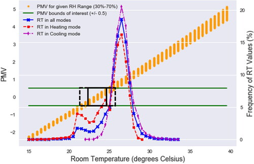
Two key observations can be made from Figure 2; first, the RT values range from 15 °C to 33.5 °C and as the RT increases, the range of PMV values also increases for the same fixed range of RH values; secondly, none of the three bell-shaped RT distributions lies completely within neither the black square nor the extended black rectangle. This affords greater discussion.

Let us assume that the HVAC operation was configured to maintain optimum thermal comfort without considering energy efficiency. In this case, the ideal situation would be that all RT values were within the comfort range of 22.5 °C–24.5 °C. To put it differently, we would expect the peak and the tails of the bell-shape distribution to lie entirely within this RT range. Figure 2, however, shows that this is not the case. Instead, considering for example the RT distribution when the HVAC is operating in heating mode, we observe that only 21% of the RT values lie in the comfort range while approximately 59% of the values lie within 1 °C of the bell shape peak value being 26.5 °C. Similar trends are shown for the cooling mode and indeed across all modes, that is to say, that the HVAC system has not been configured appropriately to optimize thermal comfort. It seems that a shift of the distribution toward the lower temperatures by 3 °C would ensure that the HVAC system would provide optimum thermal comfort for over 50% of the time.

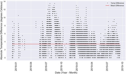
The aforementioned analysis led us to consider the difference between the RT and the STP throughout the period under consideration. The absolute difference between these two features is illustrated in Figure 3, which shows that there is a notable fluctuation between the RT and STP values. Of course, some fluctuation is expected, which would occur when the HVAC system is initially turned on and therefore require some amount of time for the RT to reach the STP, especially since optimum start functionality is not present. Figure 3, however, shows that the average difference is 3.38 °C. Worse even, the data shows that the RT reached the SPT for only 4.31% of the total recordings in the aforementioned period while the HVAC system was on. Relaxing this constraint to an RT deviation of 0.5 °C from the SPT increased the number of recordings in agreement to 13.3%, which is still very low.

Fig. 3. Difference between RT and SPT across all operation modes when the HVAC is ON.

The analysis thus far has only considered thermal comfort. Yet, a well-designed HVAC system would consider a balanced tradeoff between thermal comfort and energy efficiency. Table 3 presents different approaches for configuring the setpoint temperature. The first row shows the STP values recommended by the CEN EN15251 standards (2006) for optimum energy efficiency without considering thermal comfort. The second and third rows present the STP values identified in this work for providing optimum thermal comfort based on insights obtained from Figure 2 without considering energy efficiency. The fourth row illustrates one example of recommended STP values to achieve a balanced tradeoff between thermal comfort and energy efficiency. This recommendation is based on the thermal comfort and energy efficiency ranges identified in the previous rows and was put forward as an STP configuration that satisfies the two conditions as closely as possible.

Table 3. Comparison of different HVAC SPT approaches.

STP Approach	Heating Mode	Cooling Mode
STP for optimum energy efficiency	20.0°C (68°F)	26.0°C (78.8°F)
STP for optimum thermal comfort	22.5°C (72.5°F)–24.5°C (76.1°F)	22.5°C (72.5°F)–24.5°C (76.1°F)
STP for safe but slight thermal discomfort	21.5°C (70.7°F)–25.5°C (77.9°F)	21.5°C (70.7°F)–25.5°C (77.9°F)
Recommended STP for balanced tradeoff	22°C (71.6°F)	25° C (77°F)

Having considered both thermal comfort and energy efficiency levels, our last task was to evaluate the performance of the HVAC system taking into account the optimum values identified previously. We considered the worst-case scenario that was present in the dataset when the HVAC was operating in cooling mode. This date corresponded to the 12th of August 2019, as illustrated in Figure 4.

Fig. 4. HVAC performance evaluation in terms of thermal comfort and energy efficiency.

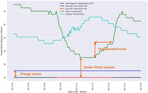
Figure 4 shows that the ideal STP value has been set to 25 °C in line with Table 3. The horizontal black and red curve depicts the SPT value set by the user on this date. The black section of this line corresponds to the period during which the HVAC system was off, while the red section corresponds to the period the HVAC was on. First, we observe that the user-defined SPT is lower compared to the ideal SPT. This implies that the HVAC is operating inefficiently in terms of energy, since it will need to “work harder” to maintain the lower SPT that has been defined. The second point is that the RT does not reach the SPT at any point while the HVAC is on for approximately 11 h between 8 am and 7 pm. Herein lies a two-fold problem; first, the HVAC system is not able to maintain the RT at the desired STP – it is clear that there is an offset of 3 °C between the RT and the STP, which corroborates the statistics shown in Figure 3; second, as a result of this inability, the thermal levels in the room lie outside the optimum comfort range. Finally, Figure 4 shows that the RT follows the same trend as the outdoor temperature when the HVAC system is off, accounting of course for a reasonable delay between the transient and steady-state periods. While it is not possible to determine the causes of the aforementioned discrepancies (since we do not have access to the system’s full information), it is clear that the data analytics process has been successful in revealing hidden trends and providing useful insights that we would have otherwise been unable to extract.

Data distribution and feature correlation

This section extends the exploratory data analysis carried out in previous work for the case study under consideration. We start by visualizing the dataset’s features split into training, validation and test sets, as illustrated in Figure 5. The features in the processed dataset include the target RT variable (top subplot), the continuous features (middle subplot) as well as the categorical features (bottom subplot) using a time-series representation. These plots are useful for unveiling trends, correlation and fluctuations in the data.

Fig. 5. Visualization of training, validation and test sets for the dataset’s features.

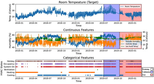
From Figure 5, it can be observed that the target variable RT has seasonality ranging from the lowest 14.0 °C to the highest 39.5 °C, that is, its values tend to fluctuate around a lower mean value in winter but around a higher mean value in summer. The RT periodically fluctuates day by day similar to outdoor air temperature and humidity, and its trend is similar to the former but with less abrupt changes. On the contrary, the setpoint temperature (SPT) remains the same during many periods with occasional changes but with an opposite trend to the RT. These observations tend to be in line with our empirical experience that the indoor RT is higher when the outdoor temperature is also relatively higher, thus leading room occupants to set a lower SPT, and vice versa.

As for the categorical features, similarities are found between the occupancy state variable and the system’s On/Off state variable. The holiday feature is periodical with certain weekly and yearly repetitions. The remaining three indicators reflect the HVAC system’s operation mode being ventilation, heating or cooling mode.

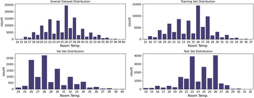
Figure 5 reveals that the target variable RT has certain short- and long-term seasonality, yet a more in-depth analysis is required. In particular, we are interested in the distribution of the target RT variable’s observations to identify whether data imbalance is present, which in turn will affect our predictive modeling choice.

Figure 6 shows distributions of the target RT observations across different sets (training, validation, test and overall) with a granularity of 1 °C. It can be seen that the distributions differ between the sets with the overall envelope skewed in different directions. Furthermore, we can observe an imbalance between room temperature classes. While the training set (top-right subplot) follows the most similar distribution to the overall dataset (top-left subplot), the RT distributions of the validation and test sets (bottom subplots) are noticeably different. It is thus anticipated that using a classification modeling strategy on this occasion would introduce severe bias in the model, which in turn would have a negative impact on the model’s robustness and accuracy. This motivated our subsequent decision to adopt a regression model for the predictive control part of this work.

Fig. 6. Room temperature distribution for each of the dataset’s subsets.

Another important contribution of this work which motivated our feature engineering process was a stationarity analysis on the target variable. To test the time series stationarity of our target RT variable, the autocorrelation coefficients and ADF unit root test are determined.

Figure 7a shows the calculated ACC and PACC of the RT series with orders ranging from 0 to 30. We observe a slow decay for the RT’s autocorrelation coefficients as the order increases, which may imply non-stationarity. On the contrary, the partial autocorrelation coefficients converge rapidly to approximately zero after the first correlation order, hence the RT is deduced to be a random-walk series whose first difference should be stationary. As a sanity check, we also evaluate the ACC and PACC of the RT’s first order difference shown in Figure 7b, where it can be seen that both the ACC and PACC converge rapidly to approximately zero after the first correlation order. This confirms our deduction that the RT itself is a random walk series because the RT series is non-stationary, yet its first-order difference is, instead, stationary.

Fig. 7. Autocorrelation plots for the room temperature feature.

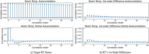
To statistically build the confidence to declare that the RT is a random walk, the ADF unit root test is applied in this case for both the RT series and its first-order difference. The ADF test results revealed that the p-values for the two series are .12 and $1.6\times {10}^{17},$ respectively. Therefore, the null hypothesis H₀ cannot be rejected for the RT series test but should be rejected for the RT first-order difference test. This means that the RT series is non-stationary, but its first-order difference is stationary. In other words, the aforementioned hypothesis test results provide further evidence that the RT series is indeed a random walk series. The above analysis motivated our decision to add the historical RT as a feature to our dataset.

Our data exploration also revealed that holidays have an impact on the RT value. It was observed that RT tends to be higher during holidays but lower during working days. Based on these observations, we added a holiday indicator as an additional new feature to our dataset which indicates whether a particular date that appears in the dataset is a public holiday (including weekends and national holidays in Greece).

Predictive modeling: results and discussion

This section presents and discusses the results obtained from the predictive modeling part of our work. Section “Performance evaluation” evaluates the performance of our XGBM-based prediction model while Section “Interpretability analysis” uses interpretability techniques including our proposed PF-FRA algorithm to explain our model.

Performance evaluation

A grid search strategy is used to fine-tune our model’s hyperparameters yielding the best candidate model on the validation set. For each decision tree estimator, the tree depth is varied between 5 and 15, the number of trees ranges from 20 to 500 while the minimum loss function reduction parameter is set from 0.05 to 2 with reasonable intervals.

A similar selection strategy is employed when determining the window width for the moving average (MVA) filter. Comparing the performance of XGBM-based RT prediction models trained with different window widths ranging from 0 to 24 h, it was found that the XGBM regressor achieves the best result with a window width of 1 h, which is thus selected as the optimum MVA window width for subsequent investigations.

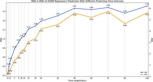
Figure 8 depicts the MSE and MAE of the predictions given by the proposed XGBM regressor over different prediction time intervals on the validation set. For practical purposes, it was determined that predicting eight hours ahead (equivalent to 48 timesteps ahead) was sufficient for the case study under consideration. Hence, subsequent analysis and discussion focus specifically on the 8-h ahead prediction scenario.

Fig. 8. MAE and MSE for RT prediction with different prediction time intervals.

Table 4 compares the performance of our XGBM model for different combinations of features ranging from just the original IOTS features through to all the features in the dataset including the new ones that were created during the feature engineering process described in this paper. For benchmark purposes, we have also included the results acquired by training an advanced neural network model, namely Long Short Term Memory (LSTM) to showcase the effectiveness of our XGBM model in conjunction with the feature engineering approach that was adopted.

Table 4. Summary of 8-h ahead RT prediction performance scores using different feature combinations.

				Metrics (Train/ Validation)
Model	Feature	Feature Number	Predicting Time Interval	MSE(°C^2)	MAE(°C)	R-squared
	Indoor, Outdoor and Time Series (IOTS)	9	/	0.9122/1.8862	0.6331/0.9883	0.9400/0.7590
	IOTS + holiday	10	/	0.8491/1.7391	0.6131/0.9665	0.9441/0.7778
	Moving averaged IOTS (IOTS-MVA)	9	/	0.9024/1.911	0.6267/0.9906	0.9406/0.7558
	IOTS-MVA + Holiday	10	/	0.8421/1.7506	0.6072/0.9580	0.9446/0.7763
	Moving Averaged Room Temperature (MVART)	1	8 h	2.3770/3.4984	1.0580/1.3484	0.8436/0.5553
	MVART + Holiday	2	8 h	1.6364/3.8437	0.9465/1.3769	0.8923/0.5089
	IOTS + MVART	10	8 h	0.4529/0.7610	0.4334/0.6106	0.9702/0.9028
	IOTS + MVART + Holiday	11	8 h	0.4252/0.7261	0.4174/0.5931	0.9720/0.9072
	IOTS-MVA + MVART	10	8 h	0.4560/0.7649	0.4367/0.6015	0.9700/0.9023
XGBM	IOTS-MVA + MVART + Holiday	11	8 h	0.4284/0.7145	0.4192/0.5805	0.9718/0.9087
	IOTS-MVA + Holiday	10	8 h	1.5224/2.2789	0.8912/1.1025	0.8998/0.7096
LSTM	IOTS-MVA + MVART + Holiday	11	8 h	0.6688/1.0121	0.5706/0.7118	0.9560/0.8707

It is important to note that all the evaluated models depicted in Table 4 are fine-tuned using the same grid search method for a fair comparison. Results show that the XGBM regressor trained with the features IOTS-MVA, MVART and Holiday indicator, has the best performance yielding an MAE of 0.5805 °C (red bold text in Table 4). This best-case scenario result is achieved using the following combination of hyperparameters; maximum depth: 11, number of estimators: 140, minimum loss function reduction: 0.05

Comparing the above model with the model trained with the features of IOTS-MVA and Holiday indicator (fourth row in Table 4 with bold text), it should become apparent that the MVART feature contributes to the model’s improved performance significantly, as evidenced by the corresponding MSE and MAE metrics. The use of an MVA filter and the Holiday indicator do improve the model’s performance compared to the variants without these enhancements, though on a lesser scale compared to the MVART feature.

Having generated the final XGBM-based RT prediction model, we evaluate and report its performance on the test set to assess its robustness on unseen data. Results show that our model achieves 1.8073${}^{°}{C}^2$ of MSE, 0.9419°C of MAE and 0.7742 of R-squared score on the test set. That means, on average, the model can predict the 8-h ahead RTs with an error of less than 1 °C. At first, this numerical accuracy might not seem acceptable with reference to sensor uncertainty (typically 5%–10% of a degree). In the context of this case study, however, and with reference to Table 3, we consider this error margin to be acceptable for the purpose of achieving a desired tradeoff between thermal comfort and energy efficiency. In terms of 1-h ahead RT prediction, the model achieves 0.4017 °C of Mean Absolute Error (MAE), which is accurate enough in most cases.

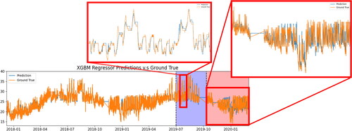
Figure 9 compares the final model’s predictions with the true RT series over the entire period with zoomed-in subplots for the validation and test sets. It can be observed that the model overall successfully forecasts the trends as well as most fluctuations though it fails somewhat for certain extreme values. More importantly, though, we observe that the predicted RT follows the true RT with little delay across all subsets.

Fig. 9. The final model’s RT predictions versus the ground truth over the entire period under consideration.

To validate our proposed method, we compare our predictive model’s performance against models that appear in related studies (Paul et al. 2018; Xu et al. 2018) which use comparable model settings and evaluation metrics. For example, these two studies apply machine-learning techniques for indoor temperature prediction and employ a feature set similar to the one described in this paper.

For a fair comparison, we introduce another evaluation metric named Mean Bias Error (MBE) which is a measure of average errors considering their signs and appears in the study by Paul et al. (2018). The MBE is calculated as shown in Equation 11(11) $$\mathit{MBE}=\frac{1\times 100}{M-1}\frac{{\sum }_{i=1}^M(y_i-f(x_i))}{{\overline{y}}_i}$$(11) : (11) $$\mathit{MBE}=\frac{1\times 100}{M-1}\frac{{\sum }_{i=1}^M(y_i-f(x_i))}{{\overline{y}}_i}$$(11)

Table 5 summarizes the comparison results of our work to the two studies mentioned above. It can be seen that our model achieves similar or better performance for short-term RT prediction. We can also see that for long-term prediction, which is not discussed in the two related studies, our model still achieves satisfactory performance.

Table 5. Comparison of our work to related studies under comparable model settings and evaluation metrics.

Research	Year	Features	Predicting time step ahead	Best model	MBE	MSE	R-squared
Xu et al.	2019	Historical RT	1	Modified LSTM	N/A	0.1424	0.8985
			6		N/A	0.4731	0.7956
Paul et al.	2018	A variety of indoor and outdoor measurements +  Time-series Feature	Not reported	Neural Network	0.6565	N/A	0.9210
Ours	2022	IOTS-MVA +  MVART +  Holiday	1	XGBM	0.0615	0.1857	0.9768
			6		0.1253	0.4048	0.9494
			12		0.1853	0.6574	0.9179
			24		0.2269	1.0808	0.8649
			48		0.1029	1.8073	0.7756

Interpretability analysis

This subsection presents the results of applying IML techniques to interpret the implemented black-box model from both global and local perspectives.

Global perspective

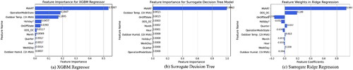
Figure 10 compares the computed feature importance/effect for the XGBM regressor, surrogate decision tree and surrogate Ridge regression models. Despite the different ranks and values for most of the features, the MVART is always the most important feature that contributes to the model decision. This result aligns with our analysis in Section “Performance evaluation” as well as our human intuition, that is, that the value of RT at a certain time depends on its previous values. Although the feature importance given by the decision tree surrogate model shows that almost only the MVART determines the forecasting logic, we deduce that this might be because the decision tree tends to overfit the training data and thus only puts the priority on the most informative feature. By further studying the mechanism through the surrogate Ridge regression which can demonstrate not only the extent but also the direction of effects for each feature, we can conclude that the MVART is the most influential feature that dominates the model’s working mechanism.

Fig. 10. Feature importance and effects for XGBM and surrogate models with significantly dominated factor MVART.

The previous interpretations focus on static analysis for feature effects in the time domain. Useful insights, however, can be extracted by examining the contribution of the features in the frequency domain. In this work, this is achieved by using our proposed PF-FRA algorithm.

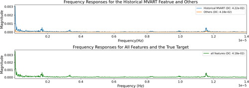
Figure 11 compares the XGBM regressor’s frequency responses (magnitude only) on the training and validation set employing the MVART and IOTS features. The spectrum of the true RT series is also illustrated for comparison purposes while the DC component is indicated in the figure’s legends. It was found that although MVART accounts for the majority of the low-frequency components, both the RT and other IOTS features contribute in a commensurate fashion to the high-frequency components. Furthermore, because the IOTS features lead to a DC component of 25.07 °C, which is closer to the original model predictions’ DC component of 25.06 °C, we deduce that the IOTS features may be more informative to determine the RT’s absolute magnitude, while the MVART contributes to the relative variations instead.

Fig. 11. Comparison of feature effects in the frequency domain for the proposed model with MVART and IOTS features using PF-FRA.

Local perspective

To analyze the chosen RT prediction model’s local behavior, we select several representative observations to conduct a sample study. The observations are from two groups, where one is the accurate group while the other is the deviated group. Observations with a prediction error less than 0.01 °C are considered as accurate predictions while those with an error greater than 2 °C are considered as deviated predictions. By means of doing so, we intend to identify why the individual prediction value varies given the same target RT value.

We carry out the analysis for two observations with the same true RT value from different groups. The two studied observations are from the test set with the same true RT value of 23.5 °C, while the accurate prediction is 23.49 °C and the deviated prediction is 20.71 °C. Two local IML techniques are applied, namely Local Interpretable Model-Agnostic Explanations (LIME) and Shapley Additive Explanations (SHAP), to verify each other’s explanation.

Figure 12 depicts the explanations given by LIME and SHAP, where (a) is for the accurate one and (b) is for the deviated one. By interpreting the explanation given by LIME, it is easy to identify that the main factor leading to different predicted values is that the MVART feature falls in different value ranges even though most of the other features have the same value. This local explanation might alert us to the fact that the XGBM-based RT prediction model could fail after a sudden change of RT values.

Fig. 12. Local explanations given by LIME and SHAP for the studied observations (accurate and deviated predictions of RT).

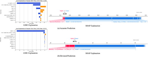
The SHAP graph provides a visualization of feature effects for the two individual observations to validate this conclusion. The force plots with the feature Shapley values show that for the two RTs smaller than the base value (the sample mean 25.06 °C), the MVART feature indeed negatively enforces the predicted value lower significantly. However, it over-enforces the deviated prediction to a further lower RT because of the lower value of MVART. Compared to the MVART feature, other features’ effects are not as significant. This result aligns with the explanations given by LIME, confirming that the historical RT information is deterministic for the model’s prediction. This leads to the recommendation that the RT prediction model is carefully supervised for the instances that the RT experiences sudden and abrupt fluctuations.

Conclusion

This paper presented a case study-based implementation of data analysis and interpretable machine learning techniques for the purpose of HVAC predictive control. Starting with a recap of previous work that analyzed thermal comfort and energy efficiency of an HVAC system in a commercial office building, the first part of this paper extended this work by considering the distribution, stationarity and correlation of the dataset’s target variable being room temperature (RT) with this dataset spanning a period of three years, enabling us to visualize trends across multiple seasons. It was deduced that using a classification model would potentially suffer from sample imbalance, thus motivating our decision to pursue a regression model instead. It was also found that the target variable is a random walk series, which in turn led us to incorporating historical RT information into our model.

Subsequently, the second part of this work explored approaches for the predictive control of an HVAC unit through the use of interpretable machine learning techniques. Results demonstrated that the proposed XGBM model can predict room temperatures eight hours ahead with an error smaller than 1 °C on average. We consider this error margin to be acceptable for the purpose of achieving a balanced tradeoff between thermal comfort and energy efficiency for the case study presented in this work.

While producing a model that can achieve accurate predictive control is of course paramount, a more important aspect and contribution of this work was to understand the working mechanisms of this model, that is to say, the logic that generates the machine-made decisions. To this end, and beyond the scope of most related studies, a number of interpretable machine-learning techniques were employed to explain the model from both a local and a global perspective. A new technique called Permutation Feature-based Frequency Response Analysis (PF-FRA), that interprets the model in the frequency domain, was also proposed and evaluated. Interpretability analysis revealed that incorporating historical room temperature (RT) values followed by moving average filtering (MVA), denoted by MVART for short, contributed the most to generating accurate predictions.

In summary, the work presented in this paper explored feature engineering, stationarity analysis and interpretable machine learning for the purpose of creating a model that could provide accurate predictive control for an HVAC unit and with the goal of balancing thermal comfort and energy efficiency. It was found, however, that the model is somewhat sensitive to abrupt RT fluctuations with some signs of overfitting. Future work will thus focus on generating a more robust and accurate machine-learning model while respecting the requirement of having sufficient model interpretability to allow the model to be trusted by human users and operators. A more ambitious goal is to deploy our model in a production environment that would enable us to assess the models’ performance in a real-world environment.

Acknowledgments

This work was completed with the contribution of General Technology Ltd., Athens, Greece, and IntelliCasa Ltd., London, UK. General Technology Ltd. provided the data for this research work. We would also like to thank the reviewers for their invaluable comments which helped us improve the quality of our manuscript.

Disclosure statement

No potential conflict of interest was reported by the author(s).

Notes

1 The code used to generate the results presented in this work has been made publicly available and may be accessed at the following Github link: https://github.com/JianqiaoMao/Interpretable-machine-learning-for-HVAC-predictive-control

References

- Agwuegbo, S. O. N., A. P. Adewole, and A. N. Maduegbuna. 2010. A random walk model for stock market prices. Journal of Mathematics and Statistics 6 (3):342–46.
- Ahn, K. U., and C. S. Park. 2020. Application of deep q-networks for model-free optimal control balancing between different hvac systems. Science and Technology for the Built Environment 26 (1):61–74. 10.1080/23744731.2019.1680234
- Alawadi, S., D. Mera, M. Fernández-Delgado, F. Alkhabbas, C. M. Olsson, and P. Davidsson. 2022. A comparison of machine learning algorithms for forecasting indoor temperature in smart buildings. Energy Systems 13 (3):689–705. 10.1007/s12667-020-00376-x
- Arendt, K., M. Jradi, H. R. Shaker, and C. Veje. 2018. Comparative analysis of white-, gray-and black-box models for thermal simulation of indoor environment: Teaching building case study. Proceedings of the 2018 Building Performance Modeling Conference and Simbuild co-Organized by Ashrae and Ibpsa-Usa, Chicago, il, USA, 26–8.
- Ariyo, A. A., A. O. Adewumi, and C. K. Ayo. 2014. Stock price prediction using the arima model. 2014 Uksim-Amss 16th International Conference on Computer Modelling and Simulation, 106–12.
- Box, G. E., G. M. Jenkins, G. C. Reinsel, and G. M. Ljung. 2015. Time series analysis: Forecasting and control. Hoboken: John Wiley & Sons.
- Breiman, L. 2017. Classification and regression trees. New York: Routledge.
- Charles, K.E. (2003). Fanger’s thermal comfort and draught models. Ottawa: Institute for Research in construction.
- Chen, T., T. He, M. Benesty, V. Khotilovich, Y. Tang, H. Cho, and K. Chen (2015 ). Xgboost: extreme gradient boosting. R package version 0.4-2, 1 (4):1–4.
- Chew, M. Y. L., and K. Yan. 2022. Enhancing interpretability of data-driven fault detection and diagnosis methodology with maintainability rules in smart building management. Journal of Sensors 2022:1–48. 10.1155/2022/5975816
- Chong, A., K. P. Lam, W. Xu, O. T. Karaguzel, and Y. Mo. 2016. Imputation of missing values in building sensor data. ASHRAE and IBPSA-USA SimBuild 6:407–14.
- Dickey, D. A., and W. A. Fuller. 1981. Likelihood ratio statistics for autoregressive time series with a unit root. Econometrica 49 (4):1057–72. 10.2307/1912517
- Du, M., N. Liu, and X. Hu. 2019. Techniques for interpretable machine learning. Communications of the ACM 63 (1):68–77. 10.1145/3359786
- Godahewa, R., Deng, C., Prouzeau, A., Bergmeir, C. (2020). Simulation and optimisation of air conditioning systems using machine learning. arXiv preprint arXiv:2006.15296.
- Grammenos, R., K. Karagiannis, and M. E. Ruiz. 2022. Analysis and optimisation of building efficiencies through data analytics and machine learning. Ashrae Topical Conference Proceedings, 1–8.
- Hall, P., and N. Gill. 2019. An introduction to machine learning interpretability. Sebastopol: O’Reilly Media, Inc.
- IEA. International energy agency (IEA), tracking buildings. 2021. Accessed September 20, 2022. https://www.iea.org/reports/tracking-buildings-2021.
- Jain, A., and P. C. Biswal. 2016. Dynamic linkages among oil price, gold price, exchange rate, and stock market in India. Resources Policy 49:179–85. 10.1016/j.resourpol.2016.06.001
- Kelly, G. E., and S. T. Bushby. 2012. Are intelligent agents the key to optimizing building HVAC system performance? Hvac&R Research 18 (4):750–9.
- Li, P., D. Vrabie, D. Li, S. C. Bengea, S. Mijanovic, and Z. D. O’Neill. 2015. Simulation and experimental demonstration of model predictive control in a building HVAC system. Science and Technology for the Built Environment 21 (6):721–32. 10.1080/23744731.2015.1061888
- Li, S., S. Ren, and X. Wang. 2013. HVAC room temperature prediction control based on neural network model. 2013 Fifth International Conference on Measuring Technology and Mechatronics Automation, 606–9.
- Little, M.A., & Badawy, R. (2019). Causal bootstrapping. arXiv preprint arXiv:1910.09648.
- Lundberg, S. M., and S.-I. Lee. 2017. A unified approach to interpreting model predictions. In Advances in Neural Information Processing Systems, ed. I. Guyon, vol. 30. Red Hook: Curran Associates.
- Mao, J., & Grammenos, R. (2021). Interpreting machine learning models for room temperature prediction in non-domestic buildings. arXiv preprint arXiv:2111.13760.
- Mateo, F., J. J. Carrasco, A. Sellami, M. Millán-Giraldo, M. Domínguez, and E. Soria-Olivas. 2013. Machine learning methods to forecast temperature in buildings. Expert Systems with Applications 40 (4):1061–8. 10.1016/j.eswa.2012.08.030
- McCartney, K., & Humphreys, M. 2002. Thermal comfort and productivity. Proceedings of Indoor Air 2002:822–27.
- Miller, C., P. Arjunan, A. Kathirgamanathan, C. Fu, J. Roth, J. Y. Park, C. Balbach, K. Gowri, Z. Nagy, A. D. Fontanini, et al. 2020. The ASHRAE great energy predictor iii competition: Overview and results. Science and Technology for the Built Environment 26 (10):1427–47. 10.1080/23744731.2020.1795514
- Miller, C., B. Picchetti, C. Fu, and J. Pantelic. 2022. Limitations of machine learning for building energy prediction: ASHRAE great energy predictor III Kaggle competition error analysis. Science and Technology for the Built Environment 28 (5):610–27. 10.1080/23744731.2022.2067466
- Myerson, R. B. 1997. Game theory: Analysis of conflict. Cambridge: Harvard university press.
- Satrio, P., T. M. I., Mahlia, N., Giannetti, K., Saito, Nasruddin, and Sholahudin. 2019. Optimization of hvac system energy consumption in a building using artificial neural network and multi-objective genetic algorithm. Sustainable Energy Technologies and Assessments, 35, 48–57. 10.1016/j.seta.2019.06.002
- Paul, D., T. Chakraborty, S. K. Datta, and D. Paul. 2018. Iot and machine learning based prediction of smart building indoor temperature. 2018 4th international conference on computer and information sciences (iccoins), 1–6. 10.1109/ICCOINS.2018.8510597
- Qin, H., and X. Wang. 2022. A multi-discipline predictive intelligent control method for maintaining the thermal comfort on indoor environment. Applied Soft Computing 116:108299. 10.1016/j.asoc.2021.108299
- Ribeiro, M. T., S. Singh, and C. Guestrin. 2016. ” why should i trust you?” explaining the predictions of any classifier. Proceedings of the 22nd Acm Sigkdd International Conference on Knowledge Discovery and Data Mining, 1135–44.
- Ruano, A. E., E. M. Crispim, E. Z. Conceiçao, and M. M. J. Lúcio. 2006. Prediction of building’s temperature using neural networks models. Energy and Buildings 38 (6):682–94. 10.1016/j.enbuild.2005.09.007
- Seppanen, O., W. J., Fisk, and O. Lei. 2006. Effect of temperature on task performance in office environment. Berkeley, CA: Lawrence Berkeley National Laboratory.
- Tartarini, F., S. Schiavon, T. Cheung, and T. Hoyt. 2020. Cbe thermal comfort tool: Online tool for thermal comfort calculations and visualizations. SoftwareX 12:100563. 10.1016/j.softx.2020.100563
- Xu, C., H. Chen, J. Wang, Y. Guo, and Y. Yuan. 2019. Improving prediction performance for indoor temperature in public buildings based on a novel deep learning method. Building and Environment 148:128–35. 10.1016/j.buildenv.2018.10.062
- Xu, Y., S. Chen, M. Javed, N. Li, and Z. Gan. 2018. A multi-occupants’ comfort-driven and energy-efficient control strategy of VAV system based on learned thermal comfort profiles. Science and Technology for the Built Environment 24 (10):1141–9. 10.1080/23744731.2018.1474690