The SLH framework for modeling quantum input-output networks

Abstract

Many emerging quantum technologies demand precise engineering and control over networks consisting of quantum mechanical degrees of freedom connected by propagating electromagnetic fields, or quantum input-output networks. Here we review recent progress in theory and experiment related to such quantum input-output networks, with a focus on the SLH framework, a powerful modeling framework for networked quantum systems that is naturally endowed with properties such as modularity and hierarchy. We begin by explaining the physical approximations required to represent any individual node of a network, e.g. atoms in cavity or a mechanical oscillator, and its coupling to quantum fields by an operator triple (S,L,H). Then we explain how these nodes can be composed into a network with arbitrary connectivity, including coherent feedback channels, using algebraic rules, and how to derive the dynamics of network components and output fields. The second part of the review discusses several extensions to the basic SLH framework that expand its modeling capabilities, and the prospects for modeling integrated implementations of quantum input-output networks. In addition to summarizing major results and recent literature, we discuss the potential applications and limitations of the SLH framework and quantum input-output networks, with the intention of providing context to a reader unfamiliar with the field.

Graphical Abstract

Keywords:

• Quantum information
• quantum control
• experimental modeling
• analysis
• quantum stochastic calculus

1. Introduction

Large scale communication and computing technologies are integral to modern life. The ubiquity of these technologies is largely due to the emergence of large scale integrated electronic circuits, which in turn are enabled by mature and powerful tools for electronic circuit design automation and analysis (e.g. SPICE, gEDA). Quantum technologies for communication and computation are being developed on several physical platforms and have the potential to one day upend aspects of these foundational information processing tasks [1]. Impressive progress in superconducting circuits, integrated quantum optics, integrated semiconductor devices, and integrated atom trapping devices [2] have led to many demonstrations of high fidelity control, measurement and state preparation in assemblies of quantum coherent systems on all of these platforms. The next step, realizing large scale quantum technologies, will require the development of sophisticated modeling and analysis tools for quantum hardware that have the same enabling capabilities as existing electronic circuit design automation and analysis tools – e.g. these tools should incorporate useful abstractions, such as modularity, networks and hierarchy, and enable coordination between high-level software and algorithmic needs and low-level hardware design.

In this review we summarize progress in developing a modeling framework, known as the SLH framework, that is capable of incorporating many of the useful abstractions listed above, and thus has the potential to form the foundation for developing tools that enable design and analysis of large scale assemblies of quantum coherent systems. The SLH framework was initially developed to model specific quantum optical networks composed of localized components that interact via itinerant, quantum bosonic fields, which we will term quantum input-output networks (QIONs). It is naturally a modular framework since each localized component is treated as a black box that the propagating fields scatter off with some pre-specified input-output behavior. In addition, it incorporates the quantum nature of the itinerant fields and any quantum dynamics in the localized components. An important aspect of using the SLH framework to model QIONs is that it enables control-theoretic analysis of such networks of quantum coherent systems, and thus facilitates the use of natural generalizations of techniques and tools from classical control theory. In particular, feedback and feedforward are naturally incorporated into the framework, which are sometimes difficult to capture within other modeling approaches. In fact, this framework is sometimes referred to in the literature as coherent quantum feedback control (CQFC) theory because the notion of modeling coherent feedback was central to its development. However, as the methodology and associated tools have developed over the past decade, it has grown into a more general framework for modeling complex networks of quantum or semi-classical systems interconnected via coherent fields (possibly involving feedback). For this reason we prefer the name SLH to refer to the framework, and the term quantum input-output network to refer to the physical apparatus being modeled.

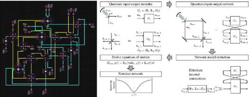
Figure 1. An example of the type of workflow for modeling complex quantum networks that is enabled by the SLH framework. Each step of the workflow is covered in this review.

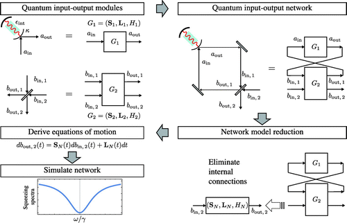
Figure 1 depicts an example of the typical workflow enabled by the SLH framework. A major goal of this review is to enable a reader new to the field to step through this workflow themselves. At the first step, individual quantum modules or components (e.g. a nonlinear optical cavity and optical beamsplitter in the upper left) are specified by triples that completely capture how the component and its internal degrees of freedom interact with input (incident) and output (scattered) fields. As stand alone modules, this description is sufficient to systematically derive equations of motion for both the field modes and internal degrees of freedom. More complex behavior and functionality is generated by connecting these components into networks, where a connection is defined as routing the output field of a module into the input field of another module, e.g. Figure 1 upper right. The SLH framework provides machinery to eliminate internal connections between the modules, resulting in a simpler, reduced model for the entire interconnected network, e.g. Figure 1 lower right. This reduced network model has the same representation as the original components, in that it is described by a single triple that captures how internal degrees of freedom interact with the remaining incident and scattered fields (not the itinerant fields making internal connections, which have been eliminated). As the entire network is now describable in the same format as its constituent components, equations of motion for the entire network may also be derived systematically from this model, such as the relationship between incident and scattered fields depicted in Figure 1 lower left. A key benefit of the universal SLH triple description of network components is that it enables many aspects of this workflow to be automated and implemented in software, thus reducing the computational burden on the user and facilitating automated design and analysis. Some fairly complicated examples of this workflow have been examined in the literature, see e.g. Refs. [3,4].

In addition to modeling networks for quantum technologies, the SLH framework is useful for modeling classical information processing networks where quantum noise in signals or components cannot be ignored. For example, at optical frequencies, an attojoule pulse contains just a few photons and thus photon shot noise cannot be ignored when modeling the interaction of such pulses with optical components. Low power classical information processing networks are becoming increasingly important as uncontrollable heat dissipation and power usage emerge as hard obstacles to scaling up the complexity of conventional integrated electronic circuits. Two important low power classical information processing applications that could benefit from SLH modeling are all-optical computers and optical interconnects [5,6].

The aim of this review is to present SLH techniques for modeling QIONs from a physics perspective. Some of the original derivations of QION results are heavily mathematical and in this review we attempt to motivate these results from physical considerations. Consequently, we will emphasize physical content and intuition, sometimes at the expense of rigorous mathematical proofs. The hope is that by emphasizing the physics, this will introduce SLH to a wider community and thus encourage wider adoption of this useful methodology and associated tools. For alternative reviews of QION theory and SLH, we refer the reader to Refs. [7–9].

The structure of the remainder of the paper is as follows. We begin in section 2 with an overview of the historical development of the SLH framework, as well as a survey of the literature on QION applications with an emphasis on some key advantages to utilizing coherent interconnects over classical signals, especially in the context of feedback systems. Section 3 reviews the basic ingredients for the development of a theory of networked quantum systems: input-output theory and the notion of cascading outputs from one system into another. Section 4 summarizes the quantum stochastic calculus constructs that naturally describe propagating fields and their interaction with localized components in a QION. The idea is not to provide a formal treatment of quantum stochastic calculus but to lay out the essential concepts with physical insight. Section 5 presents the main modeling constructs of the SLH framework, including the representation of components and rules for developing models of arbitrary networks of components. Section 6 summarizes the treatment of a subclass of quantum networks, known as linear networks, for which a number of simplifications enable the formulation of powerful analysis tools. Section 7 reviews a number of important extensions to the basic SLH framework that have been developed to expand the applicability of this modeling approach. The discussion in this section also reveals some of the key limitations of the SLH framework. Section 8 examines the application of the SLH framework to the modeling of integrated QION implementations, and some of the associated issues. In particular, we discuss in detail the application of SLH to two leading integrated platforms for quantum technologies: silicon photonics and superconducting microwave circuits. Finally, Section 9 concludes with a discussion of the outlook for QIONs and QION modeling using the SLH framework.

2. History, applications and advantages

In this section we summarize some of the historical developments and motivations in applied QION research, focusing on the literature related to the SLH framework. The literature on applications of this theory is already quite large and while we cannot survey all of it, we will attempt to point out the results that we believe will be of most interest to applied physicists. While this context is not strictly necessary for the technical discussions in the remainder of the paper, we hope that readers new to the field may find it illuminating.

2.1. History

A critical ingredient in many practical theories of complex networks is modularity. That is, one must be able to model each component of the circuit independently, and then be able to develop a model for a network of connected components without resorting to an approach where the entire network is modeled from first-principles. In electrical networks this is enabled by the lumped element treatment of electrical components, where each component is characterized by simple properties, e.g. resistance, capacitance, and the properties derived from the connectivity of the network are modeled by circuit theory without having to resort to Maxwell’s equations. However, such a treatment is not possible for optical circuits because a lumped element description of conventional optical or even integrated photonics components are invalid (optical wavelengths are much smaller than the size of optical circuit components). However, one can recover modularity by turning to scattering theory, and modeling the effect of each optical circuit component as a scattering transformation from input modes to output modes.

While such a scattering approach is routine in quantum field theory (e.g. Lehman-Symanzik-Zimmerman reduction), it was not until the formulation of input-output theory (IOT) by Gardiner and Collett [10,11] in the mid-1980s that such an approach became popular in quantum optics. As discussed more in Section 3.1, the Gardiner-Collett input-output relations relate the far-field (asymptotically free) output fields in terms of transformations of the (asymptotically free) input fields, which models an interaction with a localized system. This in turn allows one to connect the output field of one localized system to the input field of another, in a cascade configuration. This was originally realized by Gardiner [12] and Carmichael [13] in 1993, and is an important starting point for the SLH framework. The physical models that result from cascading components with interconnecting coherent fields are described in more detail in Section 3.2. Much of the motivation for developing these models was to understand the dynamics of quantum optical systems driven by non-classical light, e.g. [12,14,15]. There were a number of parallel developments in the 1980s closely related to the above formulations of input-output theory and cascaded quantum systems. In the physics community, Yurke and Denker [16] developed their own version of quantum network theory for quantized electrical circuits in the lumped-element approximation and a formalism for composing components based on electrical circuit theory. This theory has some similarities to input-output theory, and shares many of the same motivations. In addition, Kolobov and Sokolov [17] developed, from input-output theory, a special case of cascading. At the same time, a group of applied mathematicians independently discovered the mathematical objects that underlie the theory, namely quantum stochastic differential equations as rigorously developed by Hudson and Parthasarathy [18], and analyzed their properties. See Refs. [19–22] for reviews of this mathematical physics approach. The work of Hudson and Parthasarathy was motivated by the desire to write down a description of system-environment evolution (sometimes called a dilation) sufficient for generating Markovian semigroup evolution of the system. This description resulted in a coupling of the system to broadband bosonic fields that can be interpreted as the input and output fields described by Gardiner, Collett and Carmichael. This mathematical description of localized systems interacting with itinerant bosonic fields developed by Hudson and Parthasarathy was vital for the development of the SLH framework.

The first analysis of a QION that went beyond simple cascade interconnections dates to Wiseman and Milburn in 1994 [23]. They compared systems in which optical signals from a nonlinear cavity are either measured, producing a photocurrent that then controls the classical electro-modulation of the nonlinear crystal in the source cavity (measurement-based feedback control, which they termed electro-optic control), or directly routed back to the source crystal, modulating it optically and coherently (coherent feedback control, which they termed all-optical control). They discovered that the measurement-based feedback scheme was fundamentally the same as the coherent scheme when the crystal couples to only a single optical quadrature (e.g. the electric or magnetic field). This equivalence breaks down, however, when the crystal couples to both quadratures, in which case the coherent feedback scheme yields optical squeezing dynamics unseen in the measurement-based scheme. This early theoretical result suggested that quantum optical coherent feedback networks are more general than measurement-based feedback networks and that coherent feedback potentially offers new capabilities. Additionally Wiseman and Milburn’s work contained the first instance of how to algebraically model coherent feedback.

Lloyd first coined the term “coherent quantum feedback” [24] in his comparison of measurement-based feedback of a few-ion spin system with a fully-quantum feedback system in which one ion controls another set of ions. Lloyd observed that through a feedback protocol, an ion-controller was capable of generating entanglement between ions that never interact directly, while the analogous classical controller was not. This particular application was well-known, but Ref. [24] was the first to articulate that this also demonstrates that coherent feedback schemes are fundamentally more capable than measurement-based feedback control of quantum systems. While both Refs. [23] and [24] are early examples of coherent feedback control, in this work we reserve the term quantum input-output network for systems such as Ref. [23] in which itinerant bosonic fields stitch together subsystems separated by many optical (or microwave) wavelengths. These are the systems that possess the type of modularity assumed by the SLH framework.

A series of papers by Yanagisawa and Kimura in 2003 [25,26] marks the first attempt to formalize the modeling of quantum networks using control theoretic tools. The authors focused on linear quantum networks (see Section 6 for a formal definition) and described representations for network components that enable the formulation of algebraic rules for composing multiple components in series, parallel, and feedback configurations.

Then in 2009, building on the mathematical physics approach of Hudson and Parthasarathy (and somewhat motivated by IOT and Gardiner’s cascaded systems theory), Gough and James developed the fundamentals of the SLH framework as a means to compose, model and analyze networks of arbitrary (not necessary linear) components [27,28]. Following this initial formulation, there has been rapid progress in extending the SLH framework in various directions, including: relaxing approximations to make it more widely applicable, integrating control-theoretic and systems-theoretic analysis tools into the framework, and developing practical tools and software to apply the framework. In addition, there have been numerous applications of the SLH framework to model and analyze quantum and semi-classical networks. In the remainder of this review, we will describe many of these extensions and applications.

2.2. Applications and advantages

An important motivation for developing the SLH framework was the desire to efficiently model and analyze coherent feedback networks, like the one considered in Ref. [23], from a control theoretic-perspective (e.g. [29–32]). Because of this heritage, much of the literature that employs SLH models tends to focus on networks with coherent feedback, and what makes it different from measurement-based control systems, even though the SLH framework is not restricted to modeling feedback systems. For example, some of the earliest insights from applying the framework were that coherent feedback networks can fundamentally outperform measurement-based feedback networks with the same control goals. This was first observed in Ref. [31], which considered a linear-quadratic-Gaussian (LQG) control problem of a linear quantum optical system with Gaussian noise inputs (i.e. quantum noise on input optical fields). Nurdin et al. formulated a coherent feedback controller design that achieved a lower cost (a quadratic function on the magnitude of both the plant’s and controller’s fields) than the provably optimal, measurement-based feedback design [31]. Following on from this work, Ref. [33] identified the physical mechanism that enables this superior performance, namely, that coherent feedback controllers are capable of simultaneously processing both non-commuting quadratures of plant output field. By contrast, measurement-based controllers can only measure one quadrature of this output field, and thus necessarily inject additional noise when the control goal requires knowledge of both quadratures. The identification of this fundamental advantage echoes some of the insights in Ref. [23]. Similarly, Yamamoto [34] derived a handful of no-go theorems proving that linear QIONs with coherent feedback are more capable than measurement-based systems. The tasks that coherent quantum feedback enables include the generation of backaction evading measurements, generation of quantum non-demolished variables, and generation of decoherence-free subsystems (when such systems or variables are absent in the plant without the controller) [34].

Since the development of the SLH framework for QIONs, there have been a handful of experimental realizations demonstrating its validity. To date, these experiments have been implemented in free space optical and superconducting microwave systems. Ref. [35] initiated such experimental SLH studies, demonstrating the successful implementation of a fully coherent feedback loop between two free space optical cavities. The controller cavity’s dynamic response was systematically designed to reject broadband laser disturbances injected into the plant cavity. This closed loop, all-optical system was completely linear and classical, but still encapsulated much of the new, analytic machinery of the SLH model of coherent feedback networks. Extending this study, Refs. [36,37] demonstrated that experimental coherent feedback networks can also be implemented in the quantum regime, with linear free space optical networks that modified and enhanced the quantum squeezing of optical signals through coherent feedback, successfully modeled and designed using the SLH framework. Similarly, Ref. [38] (inspired by the proposal Ref. [39]) demonstrated the validity of coherent control and SLH in a superconducting microwave context with classical, digital components. Ref. [40] demonstrated digital logic gates using coherent feedback in a free space atomic and optical system. Finally, Ref. [41] demonstrated that new capabilities (tunable quality factors of cavities) could be added to the superconducting electromechanical toolbox by interconnecting two standard, “off-the-shelf” modules in a coherent quantum network.

While the fundamental benefits of utilizing QION, especially in applications that require feedback, motivate further attention and understanding of these systems, actual, future adoption of QION feedback as a common practical technique will likely depend on technical advantages, costs, and conveniences. Quantum systems are delicate and in their technological infancy, while classical controller technology tends to be mature, accessible, and commercially available. Thus, coherent feedback control – in which both plant and controller are immature technologies – and complex QIONs in general, often do not provide a clear advantage today. Most experimental applications of coherent feedback control today are more analogous to systems considered by Lloyd in Ref. [24], in which one ion controls another set of adjacent ions through near-field interactions, rather than the scattering networks exemplified by Ref. [23], that interact via asymptotically free fields. High-profile examples of these include the first repeated quantum error correction in an ion trap [42], the first demonstration of quantum error correction in superconducting circuits [43], and the near-ubiquitous use of sideband cooling in quantum optomechanics [44]. These are instances in which adjacent quantum ions, circuits, or mechanical oscillators in cavities, are coupled directly or via near-field interactions (as opposed to via asymptotically free fields). Coherent control techniques were used because of the technical expediency, rather than fundamental advantages. While classical microprocessors are capable of far more sophisticated control laws, interfacing quantum plants with a large, remote measurement-based feedback controller proved more burdensome than coupling them to technologically-similar, quantum controllers that were readily integrated with their plants. More recently, Ref. [45] experimentally studied the various technical advantages, such as feedback latency and hardware overhead, of coherent- over measurement-based control in a superconducting microwave qubit system. The QIONs described in this article rely on itinerant bosonic fields to mediate interactions between quantum subsystems, with physical separations of many optical (or microwave) wavelengths. As a consequence, the interactions between plant and controller are more separable and more modular, but are also more susceptible to decoherence in the itinerant fields (e.g. photon loss) than the direct coherent interactions (mediated by virtual photons) [42–45], and are thus more difficult to implement today. However, as quantum engineering matures, QIONs have the potential to offer the modularity and flexibility of measurement-based controllers and the integrability, speed, and fundamental advantages of direct coherent interaction schemes.

Today, proposals for QION systems typically emphasize applications in either quantum information systems, or classical information systems operating at such low energies that quantum effects become important. For example, Refs. [3,4,46] build off of direct coherent control error correction experiments such as Refs. [42,43] and continuous-time, measurement-based quantum error correction proposals [47,48] to construct autonomous, error corrected quantum memories. Emphasizing the potential to combine the natural integrability and speed of coherent feedback control with the flexibility of a networked, modular design these proposals formulate quantum networks that implement quantum error corrected memories using the 3-qubit bit/phase flip code [3], the 9-qubit Bacon-Shor [4], and a large-scale surface code  [46]. Other quantum information applications include proposals to generate remotely entangled pairs of photons [49] or qubits [50], with greater robustness to parameter uncertainty and interconnection loss by virtue of coherent feedback control.

Some researchers argue that despite the excitement over potential quantum information applications, QIONs could find more near term success in ultra-low energy classical information systems. Integrated photonic circuits have shown increasing promise in the past two decades for classical information processing applications. However, to be competitive with many electronic information systems, these photonic circuits will have to work at such low energies that fundamental quantum fluctuations (e.g. photon shot noise) will contribute significantly to signal noise and uncertainties. Many fundamental classical logic operations, such as latches and comparators, are based on integrated feedback at the hardware level, and extending such models to the ultra-low power regime demands a well-developed theory of coherent feedback networks. Many interesting questions have been recently considered in this vein including how to design digital logic gates [39], suppress the effects of fundamental, quantum noise sources [51], and accurately approximate the relevant dynamics of a large scale photonic network performing classical information tasks, but operating at quantum energy scales [52].

Finally, the concept of QIONs and the SLH modeling framework has proven to be useful for modeling fundamental properties of materials and light-matter interactions. For example, Kockum et al. have considered how to model the light-matter interaction, using the SLH framework, when atoms cannot be treated as pointlike objects [53]. This treatment has also been experimentally studied in Ref. [54]. The SLH framework has also been used to construct a QION for performing QND detection of a propagating microwave photon [55]. Another example is recent work by Brod et al. [56,57], which found a counter example to the claim that single photon cross Kerr nonlinearites cannot aid quantum computation [58,59]. Brod et al. used the SLH framework to construct a QION that models a distributed Kerr medium using a finite number of cross Kerr interaction sites.

3. Input-output theory and cascaded quantum systems

We begin the technical portion of this review by summarizing early work on modeling quantum optical networks, which can be seen as the first steps towards SLH as a more general theory of QION. Throughout this review we work in units such that .

3.1. Input-output relations

The starting point to modeling QIONs is quantum IOT, which captures the relation between asymptotic (or far-field) input and output fields that interact with a localized system, see Figure 2(a). We begin with a fully Hamiltonian description of a quantized bosonic field interacting with an arbitrary localized system:(1)

where is the Hamiltonian for the bosonic field in isolation, is the Hamiltonian for the localized system’s internal dynamics, and represents the interaction between the localized system and the field. While may remain unspecified for the moment, the field has a dense spectrum Hamiltonian in the lab frame of(2)

where are bosonic annihilation operators for the quantized field modes with units of , and satisfying canonical commutation relations . Usually, this bosonic field models a guided-wave, optical-frequency electromagnetic field mode, but IOT has also found success in modeling other systems such as microwave electrical signals and vibrational phononic modes with sufficiently low loss and at sufficiently low temperatures.¹ The interaction term is assumed to take linear form(3)

where c is a system operator and is a coupling strength between the system and field. This form of interaction is very common, e.g. in the dipole approximation of light-matter interaction [64]. Note that we are suppressing tensor product operators for conciseness, i.e. , etc.

The first assumption of IOT is that the system and bath are weakly coupled. This assumption implies that we can approximate with a simpler form. To explain this approximation, we first transform the Hamiltonian into an interaction frame with respect to the bare Hamiltonian . In this frame the interaction Hamiltonian becomes:(4)

where the tilde denotes operators in the interaction frame. We require that this interaction frame system operator take the form , for some frequency . The most obvious set of operators that satisfy this relation are operator off-diagonal in the eigenbasis of ; i.e. , where are eigenstates of . Given this form,(5)

We now make the rotating wave approximation (RWA) and drop the counter-rotating terms (the second integral in the above expression) since the oscillating integrands imply that their contribution to the evolution of the system in time will be negligible. In addition, we observe that the first integral is dominated by terms around , and hence the interaction Hamiltonian can be well-approximated by:(6)

for some frequency range around determined by .

An additional assumption of IOT is that the coupling amplitude, , has a sufficiently constant magnitude over the range , so that we can approximate in the above expression as . This is known as the Markov approximation since it ensures that the system couples uniformly to a broad band of field frequency modes, causing the field to act as a “memoryless” bath. This approximation is typically very good in systems with relatively weak system-bath interactions such that the system-bath interaction is narrowband. We additionally assume that the dynamics induced by the interaction Hamiltonian is on timescales that are long compared to , due to the weakness of the interaction and large range of bath frequencies over which the Markov approximation is valid. Under this assumption we can take to yield:(7)

Finally, since most of the dynamics in this interaction frame is centered around the frequency , it’s natural to transform the field degrees of freedom into a frame rotating at this frequency. Mathematically, this involves transforming into a frame defined by , and hence . Performing this change of frame, we arrive at the final form of the interaction Hamiltonian:(8)

Also, due to the transformation of the field degrees of freedom into the rotating frame defined by , the field Hamiltonian becomes:(9)

where in the second approximation we have formally extended the lower limit to for later convenience. Note that this does not impact the dynamics of the system significantly since and as argued above, field modes far from have negligible interaction with the system. Often we write the bath Hamiltonian as simply with the understanding that these frequencies are all detunings from .

Remark 1:

[Linear coupling] Although restrictive, the linear form of the interaction in Equation (3(3) ) is consistent with the RWA and the assumption that is very weak compared to and the relevant spectral components of . This is a particularly good approximation in optical systems in which and operate at 100s of THz and typically has GHz or lower energy scales. As a consequence, system-bath coupling Hamiltonians that are nonlinear in the bath operators (e.g. )) are ignored. In practice, while such coupling interactions may be present, they are typically dominated by linear interactions such as Equation (3(3) ) in this weak coupling limit.

Remark 2:

[Off-diagonal coupling] The other restriction in the above derivation is the demand that the elements in the coupling operator (i.e. above) are off-diagonal operators with respect to the system Hamiltonian. Although this form of the operator is restrictive, it is fairly common for light matter interactions, e.g. the dipole approximation to the minimal coupling Hamiltonian from QED. To understand this restriction further, note that we can expand any system operator as , with , and being eigenstates of . In the interaction frame defined above, all components in this sum pick up rotating factors as required for the above derivation, except for the diagonal components (or off-diagonal components if and are degenerate). The presence of such terms makes the approximations above difficult; in particular, in the presence of such terms the integrals in Equation (5(5) ) are dominated by terms around , which makes the extension of the lower limit of these integrals to invalid because the unphysical terms with significantly influence dynamics. More general derivations within the Markov approximation that include diagonal terms in the system field coupling are possible, see Refs. [65,66].

Remark 3:

[The interaction frame] We derived the approximate interaction Hamiltonian in an interaction frame defined with respect to . From here onwards we will dispense with the tilde notation since all operators will either be in this frame or the Heisenberg picture, with any exceptions specifically noted. A consequence of working in this frame is that there is no Hamiltonian for the localized system in the interaction frame. However, it is common to see the interaction frame defined with respect to only some components of the system Hamiltonian, and in such cases, one would have a system Hamiltonian remaining in this frame. An example is if the system is a two-level atom, and Then, if one chooses to define the interaction frame with respect to , then the full system Hamiltonian in this frame would be composed of Equations (8(8) ), (9(9) ), and the term (a detuning). In the following, any is assumed to be similarly defined, as the portion of the system Hamiltonian remaining after the interaction picture transformation.

Using these approximate Hamiltonians, Gardiner and Collett derive a quantum Langevin equation for the evolution of the arbitrary system operator a in the Heisenberg picture [11]:(10)

Note that here a(t) is shorthand for . This equation quantifies the influence of an input field on the dynamics of the system. The definition of the input field in terms of the field mode operators is(11)

where is the value of at the initial time . Colloquially, is the portion of the field incident on the localized system at time t. Canonical commutation relations for imply that the commutation relations for are also singular:(12)

Note that the units of are . The operators and are called quantum white noise operators by analogy with classical stochastic processes where -correlation in time implies a flat noise spectral density, i.e. white noise. The singular commutation relation of the operators and is mathematically problematic, and to remedy this smoother quantum noise increments, e.g. , will be introduced in Section 4, however we will not need these in this section.

It is often convenient to work with , the frequency domain representation of , which are related by(13)

One can also define an output field as(14)

where is the value of (in the Heisenberg picture) evolved to with . is the field at time t immediately after its interaction with the localized system (more precisely, the field at some later time , after its interaction with the localized system at time t, propagated back freely to time t). Or, more colloquially, the portion of the field scattered by the localized system at time t. Gardiner and Collett calculate the following critical relation between the input and output fields and the system [11](15)

This is typically called an input-output relation and models the effective scattering of the input modes to output modes through interaction with the localized system. Crucially, this relation allows one to calculate properties of the scattered output field once the input field and dynamics of the system operator, c(t), are known.

The spatial properties of the itinerant field have not been emphasized in the above calculation. One can also derive the input-output relation in a space-time representation of the itinerant field [64, Chap. 3.2], in which case an excitation of the field, initially at position at time , propagates to the localized system, located at , in time t. Loosely, excitations to the left of are inputs and excitations to the right are outputs, as illustrated in discrete time in Figure 2. The inputs and outputs are related by the boundary condition given in Equation (15(15) ).

In much of the following, an important mathematical object will be the unitary propagator for the system, which generates evolution of any system operator (in the Heisenberg picture), . For the dynamics described above, the propagator takes the form:(20)

Here denotes time ordering, is shorthand for the identity operator on the system and field degrees of freedom (i.e. ), and we introduce the coupling operator (note that while L is commonly referred to as an operator, it has units of ). One calculates the generator of this unitary, K(t), as(21)

We prove this form for the propagator by calculating , and showing agreement with Equation (10(10) ):(22)

To proceed, we use the following identity [11,70]:(23)

This identity is proven in Ref. [70], but we summarize the proof here for completeness. We begin by considering the commutator of the input process with the unitary propagator at the same time:(24)

Figure 2. (Left) Schematic showing the relationship between the bosonic fields defined in the text and an arbitrary localized system, in this case depicted as a cavity located at . (Right) A discrete time input-output model  [67–69].Here the boxes representing discrete input field modes that are labeled by the time they interact with the localized system e.g. , while the arrows indicate the directionality of the field propagation. The modes propagate at speed and have length . As the interaction is effectively instantaneous the field mode gets mapped to the output field as depicted at time . After the interaction the system has inprinted information on the field mode via the usual input-output relation .

Using the form of the generator given in Equation (21(21) ), we get:(25)

Furthermore,(26)

since the U(s) in this integrand depends only on input fields at times . Putting Equations (25(25) ), and (26(26) ) together yields the identity in Equation (23(23) ). Finally, substituting this identity into Equation (22(22) ), and recalling that , exactly yields the Langevin equation in Equation (10(10) ), thus validating the form of the unitary propagator given above.

For those readers who want a more detailed account of input-output theory we recommend the following references: the original papers [11,12], chapters 3, 5, and 11 of Ref. [64], and the Appendix of Ref. [71].

3.2. Cascaded systems

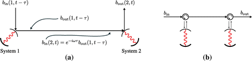
Given input-output relations for localized components we can think about what happens when the output field from one quantum optical system is routed into another. This problem was examined by Gardiner [12] and Carmichael [13] using different techniques. Both authors considered a system in which the output of a driven optical cavity feeds into another, with both cavities containing separate, nonlinear quantum subsystems (e.g. strongly coupled atoms). In the following, we will summarize the results derived by Gardiner since they relate most directly to generalizations that will follow.

Consider the setup in Figure 3 where the reflected output of a single-port cavity is fed into the input port of another such cavity. This is referred to as “cascading" the output from one system into another and is distinct from simple coupling because the probe field () is assumed to be unidirectional with no back scattering from the second cavity (this can be ensured by inserting a circulator between the two cavities, for example). Gardiner begins by writing the Hamiltonian for the intra-cavity degrees of freedom and the propagating field (in an interaction frame, and assuming the weak coupling and Markov approximations discussed in Section 3.1):(27)

where are free Hamiltonians for the intra-cavity degrees of freedom, is the arbitrary degree of freedom within cavity i that couples to the propagating field, and is the propagation time between the two cavities.

Figure 3. The cascading of the output of one cavity into another. The top mirrors of each cavity are partially transmitting, while the bottom mirrors are perfectly reflecting and therefore each cavity has only one “input" port. System 1 (2) is the cavity on the left (right). (a) is an idealized schematic, while (b) is a more experimentally accurate one that explicitly shows the circulators required to enforce unidirectional propagation of fields. The cavities could contain individual atoms or atomic ensembles, in which case the dynamics can become nonlinear. denotes the incident field interacting with system i at time t, and denotes the scattered field that interacted with system i at time t.

Using this Hamiltonian description, Gardiner proceeds to derive a Langevin equation for an arbitrary intra-cavity degree of freedom, a:(28)

where is defined exactly as before as the asymptotic input field freely propagated to the interaction region, and a is an operator representing a degree of freedom in cavity 1 or 2. We will now specialize to the limit of negligible propagation time between localized components, i.e. where . This limit is most relevant for the more general treatments that follow in subsequent sections. In this zero delay limit, the above Langevin equation becomes:(29)

We note that the approximation that the propagation time may be taken to zero is consistent with the weak coupling approximations made earlier. The dynamics of interest typically act on time scales, and as long as is much shorter than these time scales of interest, the propagation delay may be ignored. However, it is also true that relaxation of this assumption is occasionally required (e.g. cm-scale propagation distances are significant when dynamics occur at GHz rates), which will be addressed in Section 7.10.

Closer inspection of Equation (29(29) ) highlights the key difference between cascading and simple Hamiltonian coupling, namely unidirectional flow of information. For example, if a is an operator in the first cavity, all terms proportional to , , and drop out, leaving only terms proportional to , , and . Whereas, if a is an operator in the second cavity terms proportional to and are potentially nonzero, so that the dynamics are potentially driven by , , , , and . Therefore, system 2 is affected by system 1 but not vice versa, as we would expect if the probe field is unidirectional. Thus the cascaded coupling breaks time-reversal symmetry and establishes a clear direction of information flow in a network of components.

This general, nonlinear cascaded system model allows one to model the two cascaded components as one effective component. As before, we can observe that the evolution of any operator within this component (in the Heisenberg picture) is generated by a unitary propagator, . For this example, the unitary propagator takes the form , with:(30)

As before, one can confirm this form of the propagator by deriving the equation of motion , and showing agreement with Equation (29(29) ). As part of this calculation, one requires the identity (derived using the same arguments as for the identity in Equation (23(23) )):(31)

Comparing the form of the propagator in Equation (30(30) ) to Equation (20(20) ) we see that an effective model for the component consisting of the two cavities can be specified by the following effective Hamiltonian and effective coupling operator:(32)

That is, by taking the inter-cavity propagation time to zero we are able to eliminate the field degrees of freedom between the cavities and treat the composite system as a single system with internal Hamiltonian and interacting the probe field with coupling operator . Such effective descriptions of composite systems is the main aim of the framework we shall describe in the following sections. While in this case it was relatively straightforward to write the full Hamiltonian for the system, Equation (27(27) ), and derive the resulting dynamics, the framework we describe is capable of treating much more complex interconnected networks of components. In particular, we will generalize this first-principles treatment of cascaded connections, while also formulating rules for other types of connections, including feedback, which significantly extends the richness of networked quantum dynamics.

4. Quantum stochastic differential equations

In the previous sections, we derived equations of motion for single and cascaded components interacting with probe fields, which produce dynamics when integrated. It turns out, however, that proper integration is far from trivial, not just because the dynamics are complex, but because they are inherently stochastic. In this section we will summarize the use of Itō calculus to calculate these stochastic quantum dynamics.

So far, we have been fairly cavalier (nevertheless, accurate) about dealing with the broadband input fields . The mathematical description of these fields is highly singular due to the canonical commutation relations . To sidestep such singularities, let us define the time-integrated quantities(34)

and consider increments in these fields(35)

Note that the units of these increments are , and their commutation relations are for and zero otherwise. These are quantum, non-commuting analogues of the classical Wiener process and are referred to as quantum noise increments or quantum stochastic increments.

Further, by using the above singular commutation relations we can compute the following vacuum expectation values(36)

where , and is the initial state of the asymptotic input field, which is assumed to be the vacuum state of all frequency modes. The vacuum expectation values above are somewhat surprising because they state that the average value of second order products of increments of the input fields can be proportional to a first-order time increment (). This bears resemblance to stochastic Wiener increments in classical stochastic theory [72], and motivates us to think more deeply about how to integrate over such increments. Similar to classical stochastic increments, we define two types of integrals over the quantum stochastic increments :

where the time interval [0, t) has been discretized into n segments, and g is any operator in the system subspace. These two definitions of integration, the first of which is called an Itō integral and the second is called a Stratonovich integral, are equivalent in standard calculus where the increments are regular. However, since the quantum stochastic increments can vary wildly even in the limit, these two integral definitions produce different results. As such, one must specify the type of integral a quantum stochastic differential equation (QSDE), such as Equation (29(29) ) corresponds to. We refer the reader to Refs. [11,73,74] for a physics-based discussion of the differences between these two integral definitions. For a more mathematical treatment see Refs. [18–21].

In general, a QSDE derived from physical principles (e.g. Heisenberg equations of motion) corresponds to the Stratonovich integral definition. To understand why this is, note that real physical noise is never exactly a white noise process. Instead, one uses (classical or quantum) white noise as an approximation of a real physical process in some limit (e.g. white noise approximates the Ornstein-Uhlenbeck process in the vanishing correlation time limit). The Wong-Zakai theorem [75,76], and its quantum generalization [66], state that the behavior of a noise-driven physical system under this singular approximation of the real noise process is captured by a QSDE that is interpreted with respect to Stratonovich integration. This is consistent with the fact that Stratonovich differentials are consistent with standard calculus rules, while Itō differentials obey a modified chain rule:(37)

where X(t) and Y(t) are arbitrary functions of operator valued stochastic variables and and are specified in terms of Itō QSDEs. The first two terms arise from the usual non-commutative chain rule and the third term is known as the “Itō correction".

Therefore, the QSDEs we derived in the previous section for system operators (e.g. Equations (10(10) ), and (29(29) )) or unitary propagators (e.g. Equation (21(21) )) should be interpreted with respect to the Stratonovich integral (or more succinctly, we will refer to QSDEs being in Stratonovich or Itō “form"). However, QSDEs in Itō form are often much easier to work with analytically and numerically.² Fortunately, there is a straightforward procedure to convert between QSDEs in Stratonovich and Itō forms, see e.g. [64,73].

Because it will be used heavily in later sections, we write the Itō form of Equation (21(21) ) here [64]:(38)

where the term arises from the conversion between Stratonovich and Itō forms (i.e. the Itō correction). We will often write the Itō propagator U(t) as for convenience.

Remark 4:

[QSDE notation] By convention, QSDEs in Itō form are nearly always written in terms of increments (e.g. an equation for and not ). Stratonovich QSDEs are also sometimes written in terms of increments and in that case, it is customary to make explicit the Stratonovich interpretation by writing the product of a (possibly operator-valued) quantity g(t) and an increment as: .

From here-onwards, we will work exclusively with QSDEs in Itō form since the original SLH framework was developed in this form. Finally, for more detailed accounts of QSDEs from a physics perspective, we recommend the following references: Section 3.4 of Ref. [77], Appendix A of Ref. [78], Section 3.2 and Chapter. 11 of Ref. [64], and Section 3 of Ref. [76]. Additionally, Cook’s PhD thesis  [79] provides a good bridge between the physics and the mathematics literature.

5. General quantum input-output networks and the SLH framework

Despite the success of input-output theory and the cascaded approach to networked open quantum systems, the approach sketched out in Section 3 can only be used to construct networks with a small number of components due to the difficult symbolic manipulations required. Thankfully a powerful elaboration of the cascaded approach, developed by Gough and James [27,28], allows for description of large networked quantum systems using easy algebraic manipulations. In this section we will review the Gough-James formalism, which is commonly referred to as the SLH framework or SLH formalism.

The general philosophy of the SLH framework is that the dynamics of an arbitrary local quantum system interacting with an input-output channel is described by a QSDE for the propagator for the system and field degrees of freedom. This QSDE is parameterized by a triple of operators (S,L,H). The mathematics behind this is described in Section 5.1. The power of the SLH formalism lies in its ability to compose the propagator for local components according to how they are connected in a network. The mathematical rules that govern the combining of SLH systems are given in Section 5.2. From the combined propagator one can derive Heisenberg equations of motion and input-output relations for the entire network, as described in Section 5.3. In addition, a master equation describing the evolution of the internal state of all local components in the network can be derived, see Section 5.4.

5.1. The SLH time evolution operator and SLH triple

In Section 3 we saw that under the weak coupling and Markov approximations, the dynamics of an arbitrary local component, or more generally the dynamics of a cascaded system, interacting with input and output fields can be represented by a unitary propagator with some and . This turns out to be widely applicable to all components where the weak coupling and Markov approximations can be made. The SLH framework is built around a slightly more general unitary propagator than Equation (21(21) ) or Equation (38(38) ), which is traditionally written in its Itō form as:(43)

for some (interaction picture) operators S, L, and H on the localized system Hilbert space. In the remainder of this work I with no subscript will denote the identity operator on the system Hilbert space. This equation is often referred to as the Hudson–Parthasarathy equation [18]. Consistent with the previous sections, we interpret L as the system operator that couples to the external field (who’s increments are ), H is the system Hamiltonian, and S is a new object known as a scattering operator. The operator, , is an increment in the field’s number operator and its integral is sometimes called the gauge process in the literature. The gauge process and its increment are formally defined as:(44)

and are both unitless. Note that when , Equation (43(43) ) is exactly Equation (38(38) ), the Itō form of the generator we specified in Equation (21(21) ). Although we did not encounter in our discussion in Section 3, it is necessary to describe localized components that impart phase shifts on the input field, e.g. a mirror that adds a phase shift to an itinerant field. A more general interpretation of S and the gauge process will be given shortly when we consider multi-mode generalizations where each localized component may interact with multiple input and output fields. From Equation (43(43) ) it is clear that a localized component is completely specified by an operator triple (S, L, H), often termed the SLH triple. The formal solution to Equation (43(43) ) is  [19,66,80,81](45) Here we use the symbol U(t) to denote the system-field propagator in the time interval [0, t). On occasion we will need to specify a different initial time, in which case the propagator is denoted – i.e. .

Remark 5:

The physical approximations that are needed to specify a component using the unitary propagator in Equation (43(43) ) are similar to the ones required to arrive at the unitary propagator we derived from physical arguments in Section 3 – i.e. weak, linear coupling of system degrees of freedom to itinerant fields, and the Markov approximation.

When constructing large networks we will need to consider components interacting with multiple input-output modes. Multiple input-output modes may model the orthogonal free field polarization, spatial, or frequency modes that interact with localized components. Multiple input-output modes may also model bosonic free fields of different physical origins, with a single localized component coupling to itinerant optical, microwave electrical, or even vibrational phononic modes, as appropriate. When considering multimode QIONs we will suppress the subscript “" on the input fields in favor of the mode labels for notational convenience. Furthermore we will suppress time dependence of field operators unless it is essential for clarity. The QSDE description of a localized system interacting with multiple (n) input fields is given by (using Einstein summation convention, with the sum ranging over ):(46)

where is the system operator that couples to the ith input mode, H is the system Hamiltonian, are scattering operators that are constrained by the identities: and , see [82, Appendix A] and [28, Section IV] and the references therein. The input quantum noise increments and gauge process are defined as:(47)

Now it is possible to give a more general interpretation of the gauge process. represents direct scattering of photons from mode i to mode j during the time increment from t to that are not mediated by energy exchange with internal degrees of freedom of the localized components (e.g. “beamsplitter”-like scattering). When , it represents a phase shift of mode i, as in the single mode case. is a system operator that reflects the effect on the system when a photon is directly scattered from mode j to mode i.

Once again, the localized component is completely specified by a collection of S and L matrices, and an H matrix. For conciseness this can be specified in vector notation by the triple (48)

where there are n input-output ports and the operators and have dimension of the local system. The generalization of the scattering identities translate to a unitarity condition on ; i.e. (see (51)), where we have defined(49)

for any operator A. Similarly, we can define vector notation for the input fields and gauge processes:(50)

We will often refer to such systems as having n input and output ports. Let us specify some notation for these operator-valued matrices. Let(51a) (51b) This vector notation allows Equation (46(46) ) to be written in concise form as(52)

An important point to emphasize is that specifying a triple , along with an initial state of the local components and input fields in a network, completely specifies all properties of a network. This is because the way in which the operators (S,L,H) couple to the field is fixed by Equation (52(52) ), which prescribes the time evolution of all network components.

At this point, we specify some useful rules for working with the stochastic increments present in Equation (46(46) ). Since second order terms in the increments can be non-zero we must state all multiples of stochastic and deterministic increments up to second order. This is conventionally given in the form of an Itō table. When the underlying fields () are in the vacuum state, the corresponding Itō table is where we take the row and multiply by the column (row column) to obtain the resulting product under vacuum expectation. All increments are at the same time – i.e. , . All increments at different times multiply to zero.

5.2. SLH composition rules

The SLH composition rules, developed by Gough and James [27,28] are algebraic prescriptions for combining SLH triples of individual components whose asymptotic free fields are connected in various manners. These algebraic rules tell us how to simply compose networks of SLH components and can be considered the heart of the SLH framework.

Three critical physical assumptions underly these rules: (i) the Markov approximation is valid for the interaction between localized components and propagating fields, (ii) that the fields interconnecting the components propagate in a dispersionless, linear medium, and further, that the time for propagation between localized components is negligible, and (iii) the input fields into the network are in the vacuum state. Assumption (iii) might seem overly restrictive but we will see in Section 7 that non-vacuum states of the propagating fields can be introduced into the network using various extensions. Under these assumptions, the SLH composition rules are derived in Refs. [27,28]. We will summarize the rules here, and then Examples 5.2 and 5.4 illustrate the application of the rules.

Rule 1 (Series product or Cascade rule):

[Series product or Cascade rule] We begin with the cascading of the output from one localized network, represented by , into the input of another, represented by , see Figure 4. Both systems must have the same number of input fields and the ith output field of is the ith input to . We explain how to relax both of these assumptions shortly. The result of this connection, referred to as the series product of and   [27], and denoted as , is given by(53)

Note that the effective Hamiltonian for the combined system has picked up a dependence on the coupling operators for the component blocks. Note that the Hamiltonian term makes , due to the fact that the fields linking the localized components are directional.

Rule 2:

[Concatenation product] Now we examine the parallel grouping of two components with independent input-output fields and SLH triples and ; see Figure 4. The result of this parallel grouping, referred to as the concatenation product of and   [28], and denoted , is given by(58)

Figure 4. Schematic representations of the series product , concatenation product , and direct coupling which is special case of the concatenation product.

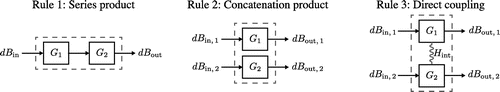
Rule 3:

[Direct coupling] The next composition rule is direct coupling, which is a generalization of the concatenation product. Consider and in parallel, and then add a direct Hamiltonian interaction between the two systems, , which is an operator on , the tensor product of Hilbert spaces of and .(59)

Then there is ambiguity in how to specify the direct coupling product. can be associated with or or symmetrically into both. We prefer to adopt the convention that the coupling resides in the first system. Recently, this composition rule has also been denoted as a “bowtie" product  [9].

Rule 4:

[Feedback reduction and network interconnection] Finally, we examine the most complicated interconnection: the feedback reduction. Given a component described by an SLH triple , the feedback reduction computes the SLH triple that results from interconnecting an output of G to an input of G. Let the original system G have n input and output ports. Let x be the output port that is connected to the input port y, we denote this interconnection by (see Figure 5(a)). The feedback reduction rule eliminates this internal link and results in a new system , where [27](60) (61a) (61b)

and the identity I has the dimesion of the reduced Hilbert space. Here the subscripts on and with overbars denote matrices with certain rows or columns removed. Explicitly,(61c) (62a) (62b) (62c) (62d)

Or in words: , and , are the (x, y) element, and the yth column, of , respectively. is without the xth row and yth column (the (x, y) minor of ). is the yth column of with the xth row deleted, and similarly, is the xth row of with the yth column deleted. Lastly, is without the xth row, and is the xth row of . Importantly, if one is eliminating multiple ports, i.e. x and y are sets, the order in which the eliminations are done does not matter. However, one must be careful about tracking indices in this case since once an input or output is eliminated by connecting it to another output or input, the correspondence between the ordering of the inputs/outputs and the row and column numbers of and must be reconsidered. We elaborate on this important issue in Remark 8, which also contains an example that illustrates how to interconnect a network by simultaneously eliminating multiple internal wires.

The concatenation product and the feedback reduction rule are sufficient to compose any number of components and construct arbitrary networks. The basic procedure to follow for an arbitrary network is to (i) form the concatenation product of all components in the network as if all components are independent and unconnected, and then (ii) apply the feedback reduction rule to implement all connections in the network. Thus the series product is a special case of the feedback reduction. However, we specify it as a separate rule since it is so commonly used.

It is instructive to examine some abstract examples to illustrate the feedback reduction rule. Our example explores the difference between Figure 5(b) and (c).Consider the feedback network in Figure 5(b), whereby output 2 is connected to input 2. An application of the mathematical prescription of the feedback reduction yields(62e) (63) Now consider connecting the output of port 1 to the input of port 2, as depicted in Figure 5(c). This results in:(64)

The difference between Equation (64(64) ) and Equation (65(65) ) demonstrates that the reduced system depends on which ports are connected in feedback.

Some intuition for the physics captured in the feedback reduction rule can be gained by examining the form of the coupling term in Equation (65(65) ): , where in the second expression we have Taylor expanded . This expansion makes it clear that the output at port 2 under the feedback reduction is a combination of and after it has gone an indeterminate number of scatterings from port 1 to port 2. The modifications to the other members of the triple under the feedback reduction can be interpreted in a similar manner.

Figure 5. Schematic representations of the feedback reduction [28]. Notice that any output port can be connected to any input port.

Remark 6:

[Padding: combing systems with unequal numbers of input-output ports] Combining systems that have different numbers of input and output ports is often required when composing SLH networks. While Rule 1 does not strictly allow this, Rule 2 comes to the rescue. The general problem is to cascade an M input-output port network into a port network and supposing that . We begin by defining a trivial SLH component, called a padding element, that simply scatters input fields directly to output fields for n modes. Generally the padding element of dimension n is denoted [85](65)

where is the length n zero vector and is the identity matrix. Now we concatenate and then cascade(66)

Remark 7:

[Permuting input-output channels: rewiring between network nodes] Strict cascading in the SLH framework leads to the ith output field of being the ith input to . If the actual interconnections are more complex it may be difficult to construct a SLH model of the network that obeys the true mapping. This difficulty can be lifted by inserting a trivial component that reorders the output fields, described the SLH triple  [85]:(67)

here denotes the permutation in relational notation, and is the permutation matrix with elements where is a Kronecker delta. Importantly this definition ensures correct composition of permutations i.e. . One can think of this component as effectively modeling the rerouting of fields between two components.

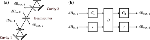
Figure 6. Network interconnection using the feedback reduction rule  [28]. (a) The network to be modeled. Note that we have a loose interpretation of which ports are considered in and out ports in this figure. (b) The same components concatenated. Here all the inputs are on the left and all the output ports are on the right. (d) To eliminate multiple internal nodes at once using the formula given in Equation (61) one must bring networks into a form where the eliminated nodes are block contiguous. We choose to have all eliminated nodes at the top of the circuit. (d) the required permutations of the input and ouput ports for the circuit given in (c) to bring it into the correct form so that feedback connections in (d) can be applied, i.e. by connecting for we obtain (a).

Remark 8:

[Network interconnection and eliminating multiple ports] There are some subtleties in applying the vector form of the rule Equation (61). We now give an example to illustrate how to interconect a network while simultaneously eliminating multiple internal wires. We wish to wire up the network given in Figure 6(a). We specify the SLH triples(68)

We form the concatenation product(69)

which is shown in the Figure 6(b). Notice that we have consistently put all input ports on the left and all output ports on the right.

To wire up Figure 6(b) to look like Figure 6(a) we would connect the following in and out ports: If one tries to naïvely apply Equation (61) the result is nosense. In order for Equation (61) to be applicable, we need to bring the network input and output ports and internal ports into a block contiguous form. One such form is depicted in Figure 6(c). The remainder of this remark illustrates how to do this for this particular example, the basic technique involes permuting the input and output ports using Remark 7.

The correct permutations for the input ports are [depicted on the left hand side of Figure 6(d)], while the ouput ports are [depicted on the right hand side of Figure 6(d)]. The corresponding scattering matricies are(70)

The rewired system, depicted in figure Figure 6(a), is(71)

where the new network SLH operator are(72)

With respect to the new wiring, we connect the following ports to correctly wire the system: This obeys the wiring convention in Figure 6(c). In the interest of being very explicit about how to do the elimination we specify the following operators from Equation (62)(73) (74a)

Substituting these operators into Equation (61), and after some matrix algebra, we find(74b) (75a) (75b)

The resulting system is quite abstract, however, we will see later that this system can be used as a way to model counter propagation in IOT, see Example 7.2 and Equation ().

5.3. Network Heisenberg equation of motion and network input-output relations

The SLH framework represents each network component as an SLH triple and the network construction rules outlined in the previous subsection specifies how to combine different components according to the network connectivity. Moreover, given a description of a network of components in terms of an SLH triple, , and the corresponding unitary propagator, Equation (52(52) ), we wish to compute the output fields in terms of the input fields.

We define the output field processes as time-evolved Heisenberg operators, where the evolution is given by the network propagator, i.e.(75c) (82)

where again, it should be kept in mind that the time label on the input processes does not indicate a Heisenberg operator at time t, but rather a temporal mode label. This definition of the integrated output field is consistent with the output field defined in Section 3, as we will show in Example . We wish to derive QSDEs describing the evolution of these output field processes, and to do so, we define their increments, e.g. , and similarly for . Expressing this increment in terms of the input fields yields [86]:(83)

and similarly for . In the second line we have defined an infinitesimal propagator from t to , and decomposed (this decomposition is possible because the dynamics is Markovian). Further, we used the fact because since the propagator from t to does not depend on any input fields at times . To obtain the form of the infinitesimal propagator we expand the formal solution Equation (45(45) ) to first order in [86]:(84)

Computing using these definitions, one arrives at the following input-output relations for the general multiple input/output case [8,9]:(85) (86)

Here, and in the remainder of this subsection, the time index on the system operators, e.g. , is meant to indicate that these are operators in the Heisenberg picture – i.e. , with , where the in the tensor product denotes an identity on all field degrees of freedom. Equation (86(86) ) is a generalization of the input-output relation in Equation (15(15) ); it specifies the output field increments as a scattering transformation of the input fields plus a contribution from the internal states of the localized components. Similarly, Equation (87(87) ) specifies the photons scattered to the output fields during the time increment from t to in terms of a combination of input photons and contributions from localized components. The following example explicitly calculates the input-output relation for a single port component, and applies it to derive the form of the output field from a cascaded network.

Next, one can derive equations of motion for operators of the localized systems in the network using the general form of the propagator, Equation (52(52) ), and the expression for the differential of a Heisenberg operator (in Itō form):(87)

For an arbitrary system operator, X(t), within the network the equation of motion becomes (using Einstein summation with all sums ranging over ) [87]:(91) We can write this equation in more compact form by overloading some notation [27]:(92)

with(93) (94) (95)

Figure 7. (a) Physical diagram of network N, modeled by Equation (). (b) SLH block diagram of network N, modeled by Equation (). The blocks labeled I are padding components as discussed in Remark 6.

For clarity, we also write the single-port versions of these input-output relations and the equation of motion:(96) (97a) (97b)

where the single-port Heisenberg picture Lindblad operator is(97c)

As a final point, we note that one may encounter the “quantum flow" notation in literature where an operator X at time t is denoted in the Heisenberg picture by(98)

Although this notation is more cumbersome, it is more precise because it makes explicit the quantities in the Heisenberg picture, e.g. in this notation the equation of motion in Equation (97c(97c) ) is(99)

5.4. Master equation description

Once the SLH composition rules have been used to derive the form of a QION, it is sometimes useful to trace over the input-output fields, and derive an equation of motion for just the localized degrees of freedom. This will result in a statistical description of the dynamics of the localized systems since the effects of the propagating fields have been averaged over by the trace operation. Since the input fields are in the vacuum state, this description is easily given in terms of a Markovian master equation for the density matrix for the localized degrees of freedom. Explicitly, we wish to compute a dynamical equation for the quantity , where is the density matrix for the entire system, and denotes a partial trace over the Fock spaces of all input-output fields. Here, consistent with the development of the SLH framework, we assume that the initial state of all the field modes is vacuum. Since the entire system evolves according to the propagator specified in Equation (52(52) ),(100)

This computation can be carried out using the facts that the initial density matrix can be factored into density matrices for the localized components and the field modes, and that the field modes are in the vacuum state; i.e. . Then using the Itō table in Equation (53(53) ), one arrives at the master equation corresponding to a general network parameterized by the SLH triple :(105)

where(106)

which should be compared to Equation (98(98) ). This is a deterministic equation of motion since the stochastic quantities have been averaged over.

In some instances not all of the output fields from the coherent quantum network are traced over. Instead, some may be monitored by detectors, and in such cases, one can write conditioned dynamical equations for the localized degrees of freedom, termed stochastic master equations, quantum trajectory equations or quantum filtering equations. This topic is reviewed extensively in Refs. [88,89]; there are great introductions in Refs. [67,89,90] and [22,69] (the first group of references are from a physics perspective, while the second group are from a mathematical physics perspective). There is also extensive primary literature on this topic, e.g. Refs. [88,91–100], and hence we do not discuss this topic further in this review.

Finally, note that the matrix does not appear in Equation (106(106) ). This is because the initial state of the field degrees of freedom was assumed to be vacuum. In Section 7.1 we will discuss QIONs with non-vacuum input fields, and see that in this case the master equation for system degrees of freedom can depend on ; see Example 7.1.

6. Linear quantum networks

Linear quantum networks, and linear quantum systems in general, are more experimentally accessible, especially in the optical regime, and thus have been extensively studied in quantum optics, e.g. see Refs. [89,101]. Linear quantum systems are most commonly encountered when dealing with collections of harmonic degrees of freedom and we will restrict our attention to this context here. In this case each degree of freedom is characterized by annihilation and creation operators () with bosonic commutation relations: . In the context of QIONs, a linear quantum network is one where the localized components are composed of harmonic modes with quadratic Hamiltonians, and linear couplings to external, propagating fields. One can also include measurements of the output fields and retain a linear system description if the measurements are Gaussian, e.g. homodyne measurement of an arbitrary quadrature or a heterodyne measurement.

In this section we will formally specify linear QIONs and define useful alternative representations of such QIONs (i.e. alternatives to the SLH triple representation). Linear systems are also extremely well studied in classical control theory and many control theory techniques have been ported from the classical linear systems context to the quantum linear systems. In Section 6.3 we will present a review of some of these techniques and results.

6.1. Passive linear quantum networks

We begin by defining a sub-class of linear quantum networks, those containing only passive components. In the quantum optics context these are networks containing components such as beam-splitters, phase shifters, and empty cavities. Consider a QION with such components, represented by an SLH triple . We can collect the annihilation operators for all degrees of freedom in the network in a vector(107) The condition that the QION is a passive linear network implies that [102] (i) the elements of are scalars, (ii) all elements of are linear in , i.e. there exist complex constants such that , and (iii) H is quadratic and conserves total photon number, i.e. there exist complex constants such that .

Given the SLH triple, one can derive equations of motion for the internal degrees of freedom represented in the vector using Equation (92(92) ) and also calculate the output fields from the QION using Equation (86(86) ). Doing so yields a set of forced linear differential equations of motion for the internal degrees of freedom and a linear relationship between the inputs, outputs and :(108) (109)

where is defined as a vector of instantaneous input field annihilation operators – i.e. (recall that ) – and a vector of output field annihilation operators. The matrices A, B, C, D are defined in terms of the elements of the SLH triple as:(110)

where is an matrix with elements , and is an Hermitian matrix with elements . For linear QIONs specifying the matrices A, B, C, D is equivalent to specifying the networks using an SLH triple. Equations (109(109) ), and (110(110) ) strongly resemble the specification of a classical linear dynamical system [103], in what is usually called the ABCD representation. However, it is important to keep in mind one distinction: whereas in the classical linear systems case the matrices A, B, C, D are independent and can be specified arbitrarily (as long as they are the appropriate dimensions), in the quantum case they are strongly dependent, as evidenced by their specification in terms of the SLH triple, Equation (111(111) ). Fundamentally, this is due to the constraints placed on quantum evolution placed by the uncertainty principle [89, Chapter 6], or alternatively due to the fact that the evolution of the composite system is unitary.

We note that one can reverse the equalities in Equation (111(111) ) in order to obtain an SLH triple given a linear system in the ABCD representation, i.e.(111)

The linear differential equation for in Equation (109(109) ) can be solved by Laplace transform, and one can get an explicit expression relating the input and output fields for the QION in the Laplace domain [82]:(112)

where , , and is the initial value of the internal degrees of freedom. In the above, we denote variables in the Laplace domain with a hat, i.e.(113)

for c(t) a time domain quantity and . The matrix is referred to as the transfer function matrix, again in analogy to classical linear systems, and it is sufficient to specify the input-output behavior of the QION.

6.2. Active linear quantum networks

The most general class of linear quantum networks admits components that are active in the sense that they do not conserve the total energy in the network (even in the absence of input and output ports). Some examples of such elements are squeezers (e.g. optical parameter oscillators) and amplifiers. In this case the dynamics of the system can no longer be described by transformation of the annihilation operators given in Equation (108(108) ), and instead we must expand the state vector to include the conjugate creation operators, i.e.(114)

An active linear QION has the following restrictions on its SLH triple [104]: (i) the elements of are scalars, (ii) all elements of are linear in and , i.e. there exist complex constants such that , and (iii) H is a general quadratic Hamiltonian that generates any symplectic transformation of the m modes, i.e. there exist complex constants such that . Similar to the passive case we define the following matrices for later use: the matrices with elements and the matrices with elements . We also define the following “doubled up” matrices:(115)

where for a matrix A denotes element-wise complex conjugation.

Figure 8. Example of a linear quantum network. The SLH and ABCD representations of this network are developed in Example . (a) shows the individual components in the network; is a degenerate optical parametric oscillator and is a beam-splitter. (b) shows the connected network with the two components in feedback configuration. (c) shows an equivalent block diagram representation of the connected network. Note that in (b) and (c), the fields labeled are not input and output fields of the connected network. We simply label the connecting links in order to clarify the relationship between the individual components in (a) and the connected network.

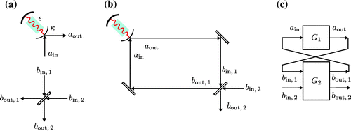
Given an SLH triple for an active linear QION, the equation of motion for the state vector and the input-output relation for the QION are also linear just as in the passive case:(116) (117)

where , and similarly for . The ABCD matrices defining the linear system are in this case [104]:(118)

where , with denotes an involution of the matrix ( is the identity matrix). As with passive linear systems, although Equations (117(117) ), and (118(118) ) resemble the ABCD representation of a classical linear system, the A, B, C, D matrices have additional constraints on them in the quantum context.

As in the passive linear network case, one can also define a transfer function matrix to capture input-output behavior in the Laplace domain. The expression for the transfer function matrix in this case is exactly the same as in the passive case but with all matrices replaced by their doubled up counterparts; i.e. and so on.

Gough et al. have specified network composition rules directly at the level of the ABCD representation for linear QIONs [104], and so one could alternatively develop a model for a linear QION using this representation for each component if it is more convenient. We note that sometimes the state of quantum linear systems is described using quadrature variables ( and ) in the state vector. In this case the form of the linear equations in Equations (117(117) ), (118(118) ) is preserved, but the definitions of the A, B, C, D matrices are modified and the input fields (that force the linear equations of motion) are also specified in quadrature form, e.g. see [89, Chapter 6]. Finally, an important feature of linear quantum networks is that they preserve Gaussian states; i.e. if all input modes are in Gaussian states, all output modes will also be in Gaussian states [105].

6.3. Survey of results regarding linear quantum networks

Due to the mathematical simplicity of linear quantum networks and their formal similarity to classical linear systems, many results concerning their dynamics and control have been derived. Summarizing all of these is out of the scope of this review, however, in the following we attempt to survey the major results. For another perspective, we refer the reader to a recent review of linear quantum networks from a control theory perspective by Petersen [107].

Some of most basic characterizations of classical linear systems are their stability, controllability and observability. Most of these characterizations carry over to linear quantum networks with little modification. For example, the notion of Hurwitz stability, captured by the eigenvalues of the A matrix, is the same in the classical and quantum regimes [104]. Controllability and observability in the quantum regime are captured by matrix rank conditions [89, Chapter 6][108] that resemble the Grammian rank conditions for classical linear systems [103].

Many of the most powerful control theory techniques in classical linear systems theory relate to optimal and robust feedback control. To understand the feedback problem, consider the sketch in Figure 8(c), where some subset of outputs of a quantum network component () are processed by another () and fedback as inputs to the original component. The fundamental question in feedback theory is how to design and realize the “controller" to achieve some control goal related to the internal variables or outputs of the closed-loop system consisting of and . An important issue that arises in the design of coherent feedback controllers is the realizability of the controller. That is, given a specification of a controller, is it physically possible to realize it in hardware using standard optical components? This is not usually an issue in classical control theory since any controller is assumed to be realizable (or can at least be approximated) using digital and analog electronics. In the quantum regime, a linear system specified in linear form, i.e. Equation (118(118) ), is realizable if and only if the following conditions are met [30,89,108]:(119)

A linear quantum system that meets these conditions is guaranteed to preserve the canonical commutation relations of the underlying system degrees of freedom, thus meeting that fundamental requirement for physical realizability.

In the quantum context, very little is known about how to design such coherent controllers. Especially challenging is optimal or robust design where the closed-loop system behaves optimally according to some criteria or has guarantees of performance robustness. When and are both linear systems, Yanagasiwa and Kimura proposed to approach the problem of controller design using the transfer function matrix description of linear quantum networks [25,26]. This was followed by two notable extensions of powerful techniques from classical linear systems control to linear quantum networks: (i) the notion of optimal feedback controllers for the linear-quadratic-Gaussian (LQG) problem [31], and (ii) the notion of robust control [30].

LQG control for a linear quantum system with Gaussian inputs aims to minimize a quadratic function of the integrated outputs, and possibly a quadratic function of the control inputs, of the closed-loop system; e.g. the cost function . Such a controller design problem is common in classical linear control theory, where it is solved by a simple convex optimization or more commonly, by determining the solution to matrix Riccati equations [103]. The solution to the quantum LQG is complicated by the realizability conditions on the controller, which are not easily incorporated into a convex optimization. However, to overcome this obstacle Nurdin et al. transform the quantum LQG controller design problem into a computationally tractable rank constrained linear matrix inequality (LMI) problem [31].

The optimal controller determined LQG controller design does not have any stability or robustness guarantees. In particular, if the model for the system is inaccurate or has uncertainties, the feedback controller may not perform as expected. A major success of modern classical linear control theory is the formulation of robust control, where the feedback controller can be designed to be robust to such model uncertainties. In Ref. [30] James et al. generalize one of the key tools from classical robust control, control to the quantum linear systems case. As with the extension of LQG control design, the key innovation by James et al. is a formulation of the controller design problem that incorporates controller realization conditions so that the resulting coherent feedback controller is guaranteed to be realizable.

Another direction in which there has been significant progress over the past few years is the controller synthesis problem. As mentioned above, there are strict realizability conditions on linear quantum systems. The coherent controller design methods described above incorporate these conditions, but even if the resulting controller is realizable, how does one construct it from basic optical components? This is the topic of controller synthesis or realization theory. Nurdin et al. established that an arbitrary linear quantum system can be synthesized by a chain of cascaded harmonic oscillator modes (e.g. cavities) with some direct, i.e. Hamiltonian, interactions between some modes, and provided a constructive procedure to determine the particular network required [109]. Later, Nurdin developed a scheme for removing the direct interactions and effectively implementing them through more complex, but completely field mediated, connections [110]. If the synthesis problem is restricted to realizing the transfer function (as opposed to the particular ABCD matrices), then Nurdin has established that this can be achieved through a purely cascaded harmonic oscillator network, for passive linear systems [111], and for arbitrary linear quantum systems [112]. It was also recently shown that several other network topologies of harmonic oscillators can be used to synthesize passive linear systems [108]. Finally, some other techniques that have been ported from classical linear systems theory to linear quantum networks are a variation of balanced truncation for linear system model reduction [113,114], and system identification for passive linear networks [115].

7. Extensions to the SLH framework

In this section we describe some extensions to the SLH framework that enable one to model commonly encountered experimental arrangements, phenomena, and imperfections. The extensions discussed involve applications of the standard SLH building blocks to capture more complex behavior such as back-reflection from interfaces, while preserving the modular network structure. In many instances, the extension boils down to approximating the more complex behavior as an interaction of freely propagating fields with a sequence of customized components. Such extensions and applications of SLH are an active area of research, and therefore the extensions we discuss are not meant to be all-encompassing. Instead, the following sections are intended to give the reader some intuition about how to model more complex phenomena using the SLH framework.

7.1. Non-vacuum input states via source models

The SLH framework relies on all field input states into the network being in the vacuum state. In particular, the network composition rules were derived using this assumption. However, in most cases encountered in practice the input fields will be in non-vacuum states. Fortunately, there are simple extensions to the framework that accommodate these situations.

The most commonly used method for accommodating non-vacuum input states is to explicitly model a network component that produces the input field state from vacuum input; in most instances this component is a minimal model for an idealized physical apparatus that produces the desired field states. The general approach is to replace an arbitrary (possibly mixed) state of the field with a system with a particular initial state and then drive it with vacuum as depicted in Figure 9. In particular we wish to engineer some fictitious “source” system and initial state of the system such that another system behaves as if it was driven by the arbitrary field state . The combination of and is often referred to as a source model. We note that developing source models and modeling a system driven with light of arbitrary statistics was Gardiner’s original motivation for developing the theory of cascaded systems [12]. Early work by Gardiner and Parkins analyzed simple two-system cascades to model driving an atom with thermal or finite-bandwidth squeezed light, and specified source models for these light sources [14]. We now summarize some of the source models that have been constructed to generate commonly encountered field states.

Figure 9. To model the driving a system with a field with arbitrary statistics we introduce a fictitous engineered source system. The source has a particular initial state at and a description in terms of an SLH triple.

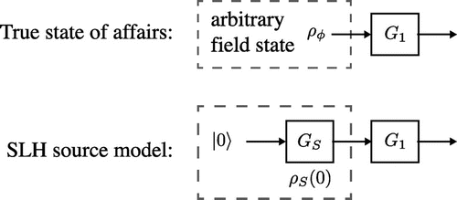
7.1.1. Coherent states

Continuous-mode coherent states provide an accurate description of pulsed laser light and are mathematically defined by [116](127)

where is the symmetrically ordered displacement operator and is a wave packet creation operator(128)

and is multimode vacuum. The square normalizable function defines the wave packet temporal profile and the mean photon number in the wave packet is [116]. For convenience we define . Continuous-mode coherent states have the eigenvalue relations(129)

This definition of continuous-mode coherent states includes single-mode coherent states ( ) and vacuum () as special cases. The displacement operator in Equation (128(128) ), also known as the Weyl operator, has its own QSDE [22](130)

This QSDE will provide an intuitive crutch for understanding the source models below.

Consider the simple, but non physical, source model:(131)

Driving a target system is simply a mater of performing the series product . This model can be understood by subsituting the above SLH triple into Equation (43(43) ). Doing so yields and since , we have exactly Equation (131(131) ). Thus when is driven by vaccum it coherently displaces the field and the output of the component is the state Equation (128(128) ). This is consistent with a Mollow transformation [117] of the output field, see Equation (159). The source model in Equation (132(132) ) allows one to easily derive the master equation for a SLH network driven by a coherent state, see Example .

A physical source model that produces this state as its output is specified by a cavity prepared in the input state with a vacuum input field and SLH triple [118,119](132)

with(133) (134)

This SLH component yields exactly the same input-output behavior as [118,119]. The first source model is usually preferred since it is numerically more efficient (the cavity degree of freedom does not need to be modeled). However, the second source model generalizes more easily and guides the development of source models for producing other field states.

Finally we note that in some cases it is important to model laser light that has finite bandwidth [120]. The usual assumption is field amplitude or intensity is relatively well stabilized so it is phase diffusion that ultimately leads to the finite bandwith. In this model we can consider where describes the phase diffusion as a function of time. If then the laser has a Lorentzian spectrum with a FWHM bandwidth of Hz [120].

7.1.2. Finite-bandwidth squeezed states

The very first paper [10], and early applications [122–124], of input-output theory were about driving systems with squeezed light. Squeezed light produced by realistic sources, e.g. a degenerate optical parametric oscillator (OPO), is bandwidth limited, typically by the transitions linewidths of the atoms in the non-linear medium. A source model for such a source is given by a cavity model with SLH triple [14,123,124]:(135)

where a is the cavity mode, is the bandwidth of the squeezed light. Note that this source is explicitly modeling the light source (degenerate OPO), and |E| is proportional to the amplitude of the pump field for this setup.

The output field from this source is quadrature squeezed with some finite bandwidth. The normally ordered quadrature variances (when E is chosen to be real and positive) are explicitly [10,14,123,124]:(143)

where the field quadratures X and Y are related to the anilation operatory by ,  : O :  denotes normal ordering of the expression O, and . In this model the Y quadrature of the output field is squeezed. Similar models can be constructed for two-mode squeezed states [125], which also implies that one can construct a source model for thermal states by simply tracing out (ignoring) one mode of the two-mode squeezed state source model [126].

7.1.3. Fock and N-photon states

A continuous-mode single-photon state is a single photon coherently superposed over many spectral modes with the spectral density function determing the weight of the superposition. In the time domain, is a square-normalized temporal wave packet, , that modulates the carrier frequency [116,127]:(144)

where . The state can be viewed as a superposition of instantaneous photon creation times weighted by the temporal wave packet. Continuous-mode Fock states in the wave packet with N photons can be constructed in the usual way [116]:(145)

and have the eigenvalue relation(146)

The temporal superposition present in Fock states means that there will be temporal correlations between different times for any system interacting with such a state. Thus systems driven by Fock states necessarily behave in a non-Markovian fashion. Using a clever source model this can be represented as a larger Markovian system.

The first cascaded model for a single photon was first discovered by Gheri et al.  [128]. This was subsequently generalized to any superposition or mixture of single photon and vacuum, ie. where and , by Gough et al.  [118]. This source model consists of a two level atom with the initial state dipole coupled to the vacuum , with given by Equation (135(135) ). The general source model for a Fock state is [119, see Theorem 2](147)

In many experimental settings one can create a state of light with a fixed photon number but it can not be written in the form of Equation (146(146) ). Such states have a definite number of photons but in an arbitrary spectral distribution function , and are called N-photon states. A general N-photon state is(148)

Then, in the time domain a general N-photon state can be written as(149)

Master equations have been derived for systems driven by this kind of field [121]. Source models for such input states exists but are fairly complicated. See the work of Gough et al., where they give a class of source models for a large family of field states termed continuous matrix product states [129]. Continuous-mode N-photon states belong to this family and in this case the source models coincide with the ones described above. However there is an interesting special case that has been solved. Consider N photons in different wavepackets, , possibly overlapping in time (e.g. a photon gun); i.e.(150)

This input state can be mimicked by a source model that is a multimode cavity with N different time dependent couplings, , to the same input-output field. This source model is detailed in Theorem 3 of Ref. [119].

7.1.4. Cat states

We shall often refer to superpositions of continuous-mode coherent states as (continuous-mode) cat states. The cat states we consider are(151)

where are coherent states, determined by complex-valued functions with if . The superposition weights are complex numbers such that the state is normalized . Constructions for the source system are given in section 4.3 of [118] and section 4 of [119]. In Ref. [118] the source model is a qudit with n levels and the L operators are projectors onto the jth qudit level with time dependent couplings given by . The initial state of the qudit, , is carefully chosen and related to and . In Ref. [119], the construction involves a multimode cavity instead of a qudit.

7.2. Alternatives to source models

In the following we will review two alternatives to source models for accommodating non-vacuum field input states. These are important because in some cases it may be difficult to construct a source model for the field driving a QION.

The first alternative to source models proceeds by decomposing an arbitrary input field into a basis that we can do quantum stochastic calculus in, i.e. one in which we can derive a master equation. If necessary, the field can be approximated by truncating in that basis. There are three bases, so far, that we can work with (1) Fock states [121,130], (2) N photon states [121], (3) a subset of multiphoton states in M modes [131], and (4) cat states [118,132]. In these bases the ordinary SLH composition rules apply. For simplicity we restrict the following discussion of this approach to a single input output mode and to Fock states.

The second alternative for dealing with non-vacuum input states aims to extend the SLH framework itself to accommodate an important class of input states: Gaussian states.

7.2.1. Simulation in a Fock basis

Unentangled Fock states, i.e. a state of the form Equation (146(146) ), span single mode Hilbert (Fock) space and form a basis for arbitrary states within the wave packet ,(152)

where , and . Using the techniques introduced by Baragiola et al.  [121] we can describe the dynamics of an SLH network described by the triple (S, L, H) when the input field is given by Equation (153(153) ). The state of the SLH node at any time is(153)

where the generalized state matrices are the solutions to a set of master equations. The set of coupled master equations are [121](154)

The initial conditions for these equations are: should be initialized with the initial system state , the off-diagonal equations, for , should be initialized to zero. Some special cases of Equation (155(155) ) were first derived in Ref. [128] and extended in Ref. [121].

To compute expectations of observables it is helpful to define the expectation value, (155)

where O is a (possibly) joint operator on the system and field. Then an expectation value of a system operator X is given by (156)

This equation also allows us to compute output field quantities; e.g. in the case of the output photon flux, taking expectations over Fock states using Equation (157(157) ) yields an equation for the mean photon flux, (157)

The solution to this equation gives the integrated mean photon number up to time t. This technique has been extended to multiple input-output modes and spectrally entangled input states in Ref. [121]. Baragiola’s thesis is a reference for this topic [133].

Finally, we note that if has a large mean field component then the Mollow transformation [117],(158) (159a) (159b)

can be used to transform away the mean field and thus more efficiently simulate in a displaced Fock basis. In addition to master equaiton methods Monte Carlo methods, i.e. quantum trajectories, can be used to simulate these equatons see [130] and the references therein.

7.2.2. General gaussian input states

Gaussian states are a wide class of field states that are particularly important because many experimental sources of light produce Gaussian states, e.g. coherent, squeezed, and thermal states. Because of their experimental relevance there are extensive reviews on Gaussian states in quantum optics and information, see Refs. [105,126,134]. Here we discuss the feasibility of incorporating these field states as inputs to a QION.

A Gaussian state in quantum theory, call it , is a state where the (possibly complex) quasi-probability distribution, e.g. Glauber–Sudarshan P function, Wigner W function, or Husimi Q distribution, is Gaussian. For a single mode this is equivalent to a density operator that is the exponential of a quadratic in the annihilation and creation operators – i.e. for  [64, see Section 4.4.5]. An alternative way to characterize a complex Gaussian state is by the first and second order moments of (the mean and covariance matrix). The relationship between these moments and the numbers is explained in  [64]. A multimode field in a Gaussian state is also characterized by its first and second moments, which can be written explicitly as:(159c) (160a) (160b)

where and . We have assumed here that the state has stationary second moments, while allowing the mean to be time-varying. The parameters N and M parameterize the covariance ellipse of the Gaussian, and are constrained by the inequality(160c)

which constrains the Gaussian state to have enough phase space area to be a valid quantum state satisfying the Heisenberg uncertainty relation. When the field is in a thermal state with thermal photons. Non-zero M indicates a squeezed state of the mode, and when there is only sqeezing and no thermal photons [64].

Remark 9:

[Squeezing parameters] When M is non zero a more convenient parameterization is in terms of physical squeezing parameters, namely and , where the parameters appear in the squeezing operator , and are known as the squeeze factor and the squeeze angle, respectively. The parameter denotes the number of thermal photons, e.g. implies . In experimental literature squeezing is usually calculated in decibels, and the conversion here is . The analysis we have presented is in the interaction picture, the relationship between this picture and the usual notion of side bands of the carrier frequency is presented in [135] and [64, Section 10.2].

The quantum Itō table corresponding to Equation (160) is(161) (162a) (162b)

Typically the mean field component is removed via the Mollow transformation [117], see Equation (159). For this reason most authors consider unless explicitly stated.

Single components with Gaussian input fields. The interaction of single localized components with white noise Gaussian fields has been extensively studied in the quantum optics literature [10,73,89,123,136,139]. In fact, the description of Gaussian fields interacting with single quantum systems has been very successful; e.g. Gardiner’s predictions  [136] of inhibited atomic phase decays in a squeezed light environment was recently verified experimentally [140]. At the core of this description is the Itō QSDE that describes the system-field evolution (under the same interaction Hamiltonian and approximations described in Section 3) when the itinerant single mode field that the system interacts with is in a Gaussian state [11,73,138]:(162c)

with , and the increments satisfy the Itō table Equation (162), H is the localized component’s Hamiltonian, and L is the operator that coupled with the itinerant field mode. Generalization of this propagator to the case of multiple input-output modes is straightforward because the input fields are orthogonal; i.e. it effectively amounts to adding an index “i" to L, , M, and N, and summing over i. Using the general relation between input and output fields, Equation (84(84) ), one can show that the input-output relations remain unchanged under this propagator. However, the equation of motion for a system operator X, is modified to (cf. Equation (97c(97c) )):(163)

This equation of motion gives rise to the master equation for localized degrees of freedom:(164a)

While this master equation is not written in Lindblad form it can be brought into such form via diagonalization  [138]. As for the vacuum input master equation, Equation (106(106) ), there exist homodyne and heterodyne unravellings of this master equation, i.e. stochastic master equations or quantum filters, see [77, Section 4.4.1] and [89, Section 4.8.2].

Note that there is no S matrix in Equation (163(163) ), and thus this equation does not capture pure scattering dynamics. This is partly because such dynamics were not of concern when the equation was derived [11,73,138], but as we will discuss further in the next section, there are some fundamental obstacles to incorporating pure scattering dynamics in the presence of arbitrary Gaussian input fields.

Quantum networks with Gaussian input fields. In the spirit of cascaded systems one can also seek to model the dynamics of a quantum network of localized components that is driven by Gaussian fields. Two studies that have examined this are Ref. [14], which considered cascading cavities, atoms, and beamsplitters driven by thermal and squeezed fields, and Ref. [23], which considered systems in series and feedback configuration driven by Gaussian fields. However, these studies construct the network dynamics manually on a case-by-case basis, like we derived the dynamics of a cascaded system in Section 3.2, i.e. by relating the output field of one component to the input field of another. Of course, it would be more desirable to have a general and systematic approach that prescribe algebraic rules for constructing network components.

In response to this, Gough and James have examined the extension of the SLH framework to treat general Gaussian input fields [70]. They demonstrate that one can model series and feedback connections using the standard SLH rules, see Section 5.2, even when input fields are arbitrary Gaussian fields. However, this comes at the cost of a reinterpretation of the dynamical equations implied by the resulting SLH triple for the network. Gough and James show that the SLH triple for the network, when the input fields are in non-vacuum Gaussian states, should be interpreted in terms of a corresponding Stratonovich QSDE. In other words, while in the vacuum input case, an SLH triple (for an arbitrary network of components) implies the Itō QSDE Equation (52(52) ) for the system propagator, and a corresponding Itō QSDE for system operators within the network, Equation (92(92) ), when the network inputs include arbitrary Gaussian fields, the dynamical equations that correspond to the SLH triple for the network (constructed using the normal SLH composition rules) can only be written in Stratonovich form (the “representation free form" of Ref. [70]). Note that one can write down an Itō form of these dynamical equations (every QSDE has Itō and Stratonovich forms), but as shown in Ref. [70] these Itō equations become dependent on the exact state of the input fields. More explicitly, in the Itō form the L members of the SLH triple carry information about the state of the input fields. This runs counter to the modular philosophy of the SLH framework, which requires the description of network components to be independent of input fields fed into them – these descriptions should capture intrinsic properties.³ In fact, this state of affairs is already hinted at by the form of the propagator in Equation (163(163) ): writing down an SLH triple that generates this propagator would lead to a dependence of the L operator, which is meant to be property of the system alone, on the field state (parameterized by N, M).

A further restriction that one encounters when accommodating non-vacuum Gaussian input fields directly into the SLH framework is that the network components cannot include arbitrary scattering matrices, i.e. . Gough and James demonstrate an approach for effectively modeling simple static beamsplitter scattering that is consistent with non-vacuum Gaussian inputs (also see Refs. [14,23] for prior work on this topic), but arbitrary scattering components are not compatible with the approach developed in Ref. [70]. In other words, there is no generalization of Equation (163(163) ) that captures arbitrary scattering dynamics.

To summarize, the results of Ref. [70] imply that if one requires (i) a modular description with components capturing only intrinsic properties, (ii) general composition rules for these descriptions, and (iii) a direct representation of non-vacuum Gaussian input fields (i.e. not through source models), then one must interpret the SLH triples in terms of corresponding Stratonovich dynamical equations.

Finally, we note that the results in Ref. [70] are consistent with observations made by Gardiner and Collett on the limitations of Itō QSDEs [11, Section III.D] . Specifically, these authors mention that defining an Itō QSDE requires knowledge of the input fields to the network, while Stratonovich QSDEs are independent of the input fields.

7.3. Emission and propagation losses

In the context of waveguides or free space experiments we call field modes that interact with the network components “guided modes”, and imperfections that couple quanta into “non-guided modes” losses. The usual technique to account for losses is to introduce a fictitious mode to represent all the non-guided modes and trace over that mode at the end of the analysis. For example, while an ideal single-port cavity is represented by the SLH triple , a cavity with losses is modeled by the addition of a fictitious port (with vacuum input). This is captured by the concatenation product , where , with being the rate of loss from the principal cavity mode.

While this introduction of a fictitious mode to capture losses is sufficient for many situations, it should be noted that one has to still be careful about modeling choices. For example, an atom coupled to a cavity field could emit into non-guided modes directly (spontaneous emission) or via a cavity mode, or via both mechanisms. In such cases, the fictitious mode (or modes) should be introduced in a way that is consistent with the physics.

Furthermore, loss in waveguides or during free-space propagation can often occur in a distributed manner. We discuss the modeling of distributed properties in more detail in Section 7.7, but note here that such losses are nearly always effectively captured by the incorporation of one or a collection of fictitious beam splitters with vacuum input (which is effectively introducing fictitious output ports to the propagation channel).

7.4. Circulators

As we have previously discussed, circulators (or isolators) are common components in QIONs that enforce the unidirectional propagation of fields. Since input-output theory and the SLH framework assume unidirectional fields, ideal circulators are implicitly present on many connections. However, real circulators have many non-idealities, including loss, imperfect isolation and finite bandwidth.

In this section we will develop an SLH model for a symmetric and lossless 3-port circulator. The lossless characteristic means that the total input power is a conserved quantity, i.e. all input power is transmitted to one of the output ports. Loss can be incorporated into this model by appending fictitious beam-splitters at each output port, for example, see Section 7.3. The circulator non-idealities we consider include imperfect impedance matching (resulting in backreflections) and imperfect isolation (routing of the signal to the wrong port of the circulator).

In the infinite bandwidth limit, a general (potentially non-ideal) circulator can be modeled by an SLH component of the form , where the three port unitary S-matrix is(165)

where the subscripts on label the scattering from port i to j. In the case of an ideal three port circulator this matrix becomes(166)

The ideal circulator maps the input fields to output fields in the following way(167)

If the circulator is symmetric but not perfect we have , , and [141]:(168)

with complex transmission, reflection, and isolation error coefficients t, r, and b, respectively. These coefficients must obey and as the S matrix is unitary [141]. The non-idealities of the circulator are then captured by the parameters [142]:(169) (170a)

Clearly is desirable.

Another circulator non-ideality that has been modeled is finite bandwidth, since real circulators are only non reciprocal devices over a finite frequency bandwidth. SLH models for finite bandwidth 3 port [143], 4 port [144], and more general circulators  [145,146] have been given in the literature. The three port model consists of three coupled cavities [143] and has the SLH triple:(170b)

When and this model behaves as a circulator for carrier frequencies close to the cavity frequency. As the magnitude of is increased the circulator becomes higher bandwidth. After adiabatically eleminating the entire Hamiltonian, see Section 7.6, one can show that Equation (171(171) ) reduces to Equation (167(167) ) upto phases which can be absorbed into the input-output operators.

7.5. Bi-directional waveguides, back-reflections, and finite length propagation

Input-output theory inherently describes one way propagation of fields. Consequently the SLH framework is built upon the assumption of unidirectional propagation of fields between components in a network that are very close to each other. Unidirectional propagation is often also referred to as chiral propagation in the literature, e.g. [147]. However, many experiments have bi-directional propagation of fields, e.g. from reflection, or impedance mismatches at node interfaces such as circulators, and finite propagation delays between components. Here we will describe how to construct an SLH model to capture bi-directional propagation on a waveguide and finite propagation distance in increasing generality.

Naively cascading multiple input output networks results, typically, in fields that are co-propagating through a network. Consider the SLH construction where we cascade the right and left going modes and then concatenate these modes, i.e.(171) (172a)

with the modeling coupling of localized components to right-propagating/left-propagating fields. The total system is them composed as . Note that one must be careful not to double-count the internal Hamiltonians of the components when forming this product. This construction lets one simulate systems such as the one depicted in Figure 10 and other slightly more complicated arrangements [56,57]. We illustrate this point in Example 7.2. In general one needs to use the method explained in Remark 8 to model counter-propagation.

In cascading quantum systems we are assuming that the systems are close enough that the propagation delay between then (e.g. Figure 3) goes to zero, and the output field arrives at the next component with the same phase. One methods to account for finite propagation distance, call it L, between the cascaded elements is to introduce a phase shift between SLH components [148]. The phase shift element is(172b) is the detuning from the carrier frequency, and the speed of light in the medium is . For many components and different distances many phase shifts are required. This treatment is only valid for small delays in propagation, where the delay is small compared to the timescales of system dynamics (typically of order ), or more precisely in a regime where . See Section 7.10 for solutions for modeling time delayed propagation outside this regime. The introduction of the phase shift can lead to nontrivial coupling between the cascaded systems, see e.g. Ref.  [148], we demonstrate this in Example 7.2.

Figure 10. A physical waveguide can have right and left propagating modes. In order to capture this in a SLH model we introduce two input-output modes. To model the finite propagation length, L, between the stationary atoms we introduce a phase shift where which is proportional to the detuning from the carrier frequency the length and the speed of light in the medium . This simplification is only valid in the Markov approximation when the delay is neglibile compared to the atomic response time. Not all two mode SLH models capture counter propagation Example 7.2 discusses this distinction in more detail.

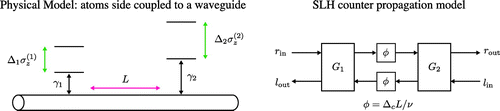
The construction above is not general enough to account for counter propagation in a general network. Importantly, the feedback reduction Rule (4) lets one connect networks with an arbitrary topology, thus we could also model counter propagation using this rule.

7.6. Model reduction by adiabatic elimination of fast degrees of freedom

Model reduction is the process of approximating a complicated model by an analytic and or computationally simpler model. Adiabatic elimination is a form of model reduction applicable when there is a seperation in timescales for different system variables. For example, consider an input-output field coupled to a one sided cavity with the cavity mode coupled to a two level atom. If the cavity is very leaky, the cavity typically equilibrates to the input field and atomic state on a time scale faster than the time scale over which either the input field or atomic state varies. Thus, the cavity state is primarily a dependent variable on the input and cavity states and need not be tracked for an accurate dynamical model. In such cases, one says that the cavity may be adiabatically eliminated.

Adiabatic elimination has a long history in quantum and atom optics. As expressed by Gardiner, the aim is to find a “method by which fast variables may be eliminated from the equations of motion in some well-defined limit" [154]. This is typically achieved by using a projection operator approach [154–157]. With respect to the QSDEs for the propagator and the SLH framework adiabatic elimination was rigorously formulated in a series of papers by Bouten, Silberfarb and van Handel [158] and [159]. The approach used in these papers is to first define a network node with some parameter k that scales the fast dynamical rates . Each , , and operators on a Hilbert space . Then, the adiabatic elimination procedure is applied which results in a node that approximates the original network without the k dependence , i.e. operates at slow dynamical rates only. Here, each S, L, and H operate on , which is a subspace of such that , where is a projection operation. Specifically Bouten et al. prove that the unitary generated by converges to the unitary generated by the network G in the following sense(173)

for all , where is the symmetric Fock space for the fields coupled to the system, provided certain – yet to be stated – preconditions hold. We remark below on the choice of .

Identifying (S, L, H) first starts by defining a QSDE for which depends on the fast timescale k:(180)

ultimately this will limit to a propagator defined by:

For the adiabatic elimination procedure to hold, the pre-elimination operators must have the following dependence on k (181) (182a) (182b)

for some operators . The physical interpretation of the k-dependance of these operators is as follows. Operators that depend on generate the fast dynamics that we wish to eliminate. The operators that have no dependence on k generate the slow dynamics, and the operators that depend on k couple the fast and slow timescales.

Adiabatic elimination is allowable in the limit , i.e. in the limit where the fast quantities tend to adiabatically “follow” the slowly varying quantities. In this limit, the operators limit to(182c) (183a) (183b) (183c)

The assumptions for this limit to hold are(183d)

For more technical details on these conditions, “Assumptions 2 (Structural requirements)" of Ref. [159] and Assumptions 3 and 4 of Ref. [158]. We note here that one has to make a judicious choice of for these conditions to hold, and this choice is often aided by physical insight into the dynamics of the network. Intuitively the projection operator acts on and projects on to the slow dynamics , while is a projector onto the fast dynamics . Bouten and Silberfarb suggest that should be thought of as the ground state subspace of and is the excited state subspace. For a mechanical method of finding the relevant operators in terms of the projector see remark 10.

Figure 11. Commutativity of adiabatic elimination (A.E.) and network composition rules.

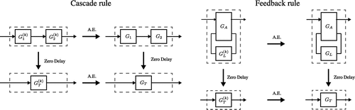
Figure 12. An example of taking a continuum limit of an SLH model from Refs. [174–176]. In this example N cavities with possibly different decay rates and resonance frequencies are cascaded. The top panel shows an experimental schematic, the first cavity is located at and the last at . The second panel is the discrete SLH model for the top panel. In the third panel we have taken a continuum limit, to obtain an SLH model that can represent a continuous medium.

In the context of a large QION, clearly if we can eliminate some parts the model will have reduced complexity model which should reduce simulation costs. The first application of adiabatic elimination within the context of a QION was by Warszawski and Wiseman [160] to simplify the dynamics of a optical feedback network (although this work predates the SLH formalism and the adiabatic elimination technique outlined in this section, and therefore applied a less rigorous adiabatic elimination technique). An important question arises when applying adiabatic elimination to simplify QIONs. Are the network dynamics different if we (1) perform adiabatic elimination on individual network nodes and then apply the concatenation, series and feedback product rules or (2) apply the rules to compose the network and then adiabatically eliminate? The fact that these two approaches produce the same result was first established by Gough et al.  [161], and then in full generality by Nurdin and Gough [162]. Intuitively these authors show that the two different pathways from the top left corner to the bottom right corner in the schematics shown in Figure 11 result in the same SLH parameters.

There can be subtleties in the elimination process. For example, when one attempts to use the above procedure to scale the amplitude of a coherent state field input (which corresponds to the parameter k for this example), mathematical complications can arise. A procedure to overcome this difficulty was developed by Bouten (unpublished) and applied in [84], and generalized in the supplementary material of [4, Section II C ]. For further explicit examples and applications of this adiabatic elimination technique see the Supplementary Information section of Ref. [3] and Ref. [163,158,159,164,165].

Remark 10:

[A quick way to find , and in Equation (182)] In practice it can be tricky finding the operators , and in Equation (182). Here we describe an intuitive method to find these operators. The method relies on using the projectors onto the ground space and the excited space to define the operators of interest. This of course requires some intution about , perhaps obtained by physical insight or numerics. We begin by denoting operators before elimination (or any k scaling) with a bar e.g. (). Now conside the following decomposition (compare with Eq. (182) which has the k dependence ) The operator Y will be eliminated in the procedure so it is in the excited space, while the operator A couples the excited space to the ground space, and B is entirely in the ground space. This suggest the following definitions(184)

With similar reasoning for and we define(185)

Clearly the treatment of the term that scaled as k in the original teratment, is different between Equation (185(185) ) and Equation (186(186) ). This is so that assumption (3) in Equation (184(184) ) holds. Note that does not depend on k or . One should also note that our choice for is different to that of the related method of Reiter and Sørensen [166].

7.7. Modeling distributed transformations

The SLH framework is fundamentally based on a modular approach that models transformation of propagating fields by a network of discrete components. However, in some cases the properties and transformations we wish to model are distributed in space. For example, understanding the propagation of light through engineered nonlinear crystals [167–172] requires modeling distributed transformations of propagating fields. In this section we discuss an approach to adapting the SLH framework to study the propagation of quantum fields through a continuous medium. This has been done many times in IOT, see for example the work of Caves and Crouch [173]. The essential strategy is to approximate the transformation as a large number of discrete components effecting infinitesimal transformations and then take a continuum limit of the cascaded model.

We take as an example the work of Hush et al. [174], which analyses a gradient echo memory using the SLH framework. A gradient echo memory is essentially a spatially distributed atomic ensemble. To model this with an SLH network one imagines the atomic ensemble as broken into thin slices, where the output of one slice is the input to the next slice, see Figure 12. All slices contain a collection of atoms with different detunings, but the slices are considered so thin that there are no emission then re-absorption events within a single slice. In this weak excitation limit it can be argued that the resulting interaction with the atomic ensemble can be approximated as a coherent exchange with a bosonic degree of freedom and modeled using harmonic oscillator raising and lowering operators [174–176]. Under this approximation, the slices formally resemble a collection of cascaded cavities, and the SLH triple that captures the dynamics induced by the k’th thin slice of the ensemble is:(186)

where is the coupling constant between neighboring slices/cavities and and are the annihilation and creation operators for cavity mode k, and . Cascading N such components results in(195)

In principle we could now write down for the entire system or work out an equation of motion for some operator K. However, we are interested in the continuum limit of this approximation, and to take this limit we recall how this modular model relates to spatial coordinates. Imagine the first slice/cavity is located at and the last slice/cavity is located at . Then the k’th cavity is located at where . In the continuum limit , becomes and the sums in Equation (196(196) ) become integrals:(196)

where . To understand the transformation of the input field implemented by this continuum model, consider the input-output relation for the network, namely . In order to characterize the output field we need to solve for , which in turn involves solving for the local modes a(x, t). Since the overall network model is linear we can easily write the equation of motion for as [174](197)

and solve it for some initial conditions. This is done explicitly, using Laplace transform techniques, by Hush et al. to study gradient echo memories  [174], single photon production [175], and cross phase modulation of photons in two gradient echo memories [176].

This notion of modeling material properties using the continuum limit of an SLH network is relatively unexplored and has significant potential.

7.8. SLH and scattering theory

The SLH framework is a route to modeling the internal dynamics of a QION and also to determine the relationship between the input and output field to the network. The output fields are specified by Heisenberg equations of motion for the canonical operators for these fields, i.e. Equation (86(86) ), and it is in principle possible to characterize the state of the output field by calculating moments of these canonical operators. However, one can exploit the connection between the SLH framework and scattering theory to make direct connection between the states of the input fields and states of the output fields. The central quantity that enables this in scattering theory is the scattering matrix, or S-matrix,⁴ which is a unitary matrix that connects asymptotic input and output field states: , where and are asymptotic field states that are usually specified as energy eigenstates of the free Hamiltonian. In this section we briefly summarize the relationship between SLH and scattering formalisms. A detailed account of this relationship can be found in Refs. [177–179] and a summary of recent scattering work can be found in Ref. [179].

We consider the interaction of a localized component with a single input-output mode, the generalization to many input-output modes is straightforward but cumbersome. The elements of the S-matrix in the frequency domain is specified by . The S operator is equivalently the propagator in the interaction picture with the following limits(198)

in this expression and where are from Equation (1(1) ). An alternative way to describe the S operator is with the Møller wave operators , where . The Møller operators map states of the system plus field to the infinite past or future and are denoted by:(199) (200)

where are eigenstates (of the field and system subsystems) of the free Hamiltonian and are “scattering eigenstates" of the interacting Hamiltonian, i.e. and . A key assumption that we make is that the system is in its ground state in the asymptotic regime, i.e. in the infinite past and future. Extensions to scattering theory that go beyond this assumption are possible, but we will not cover them.

The S-matrix elements in this notation becomes(201)

The next task is to relate this object to the input-output theory and more generally to the SLH framework. The time domain input and output fields in the asymptotic past or future, that is Equation (11(11) ) and Equation (14(14) ), are the limit where and . These can be related to the frequency domain representations by a Fourier transform – as was done in Equation (13(13) ). The Møller operators act on Heisenberg-picture operators in the following way , and . In other words, the Møller operators propagate the field operators in the asymptotic past to the interaction region, or from the interaction into the asymptotic future. Using this relation between the field operators and the Møller operators, we can deduce that:(202) (203)

where we define as the vacuum state of the field and the ground state of all components in the network. These expressions finally allow us to relate the input-output field operators in the frequency domain to the scattering matrix:(204) This expression links the elements of the scattering matrix to the input and output fields specified by input-output theory, or more generally, the SLH framework. The following example illustrates how one can evaluate the right-hand-side of this relation to calculate the scattering matrix using the input-output relations derived from an SLH description of a QION.

The utility of casting the scattering calculation within SLH framework is that one can now calculate, in principle, the S-matrix representing scattering off an arbitrary network of quantum components described by an SLH triple [181]. Indeed, recently a number of authors have recently used the SLH framework to analyze complex scattering calculations [57,182]. Notably, Caneva et al. have recently shown how to include finite spatial distances between scattering elements in a SLH network, and include propagation delays discussed in Section 7.10 [150]. The simplest solution is to cascade propagation-length dependent phases between components as explained in Section 7.5 and Example 7.2. The solution developed in Refs. [150,183] shows that there is an intimate relationship between solving the scattering problem and the generalized state matrices defined in Ref. [121]. More generally the scattering problem can become complicated when bound states are involved see e.g. [184].

7.9. Dispersive propagation

As stated in Section 5.2, two of the underlying assumptions behind the SLH framework is that the fields connecting localized components propagate in a dispersionless medium, and that the time for propagation is negligible.

The the finite propagation delay part of the assumption is treated in Section 7.10, but here we discuss dispersion. First we note that it is not a problem for the localized components to introduce dispersion; that is captured by IOT and the SLH framework. The SLH assumption is that there is negligible dispersion while propagating between localized components, and while this assumption is valid in free space, bulk optics setups, it can be violated in integrated implementations where guiding media can be dispersive. For example, silicon photonic waveguides can exhibit waveguide dispersion and material dispersion. The former is present if the waveguide’s guiding properties depend on the light wavelength, and the latter arises from dependence of the material’s refractive index on the wavelength. Both types of dispersion can be minimized by waveguide engineering, e.g. [185–187], however, removing all dispersion can be challenging.

Stace et al. have noted that dispersion can cause significant modifications to input-output theory, and have assessed the impact of this on quantum state transfer protocols [188]. We revisit their analysis to understand the effects of dispersion on the dynamics of QIONs. First, let us return to the derivation of the dynamics of a cascaded network in Section 3.2, and the Hamiltonian for the cascaded cavity example, Equation (27(27) ). This Hamiltonian is in the Markov approximation. For our purposes, let us write the interaction part of the Hamiltonian without this approximation:(205)

Recall are operators acting cavity i degrees of freedom. In addition to relaxing the Markov approximation (under which ), we have also been more explicit about the fields that the cavities interact with: cavity 1 (2) interacts with the field at location . In the dispersionless propagation case, , where and v is the speed of propagation in the medium, and thus we could omit the spatial index. However, now that we are considering dispersion, we must be more careful and therefore explicitly denote the field’s spatial index.

To understand the effect of dispersive propagation, we will express in terms of assuming quadratic dispersion, , where v is the speed of propagation in the medium and is a constant. Inverting this relation we get: , and the group velocity of waves under this dispersion relation is given by(212)

where is the carrier frequency. Under quadratic dispersion, Stace has established that the effects of dispersion on the propagated field in (t, x)-space can be modeled by a delay and convolution with a channel transfer function [188,189]:(213)

where denotes convolution and . The transfer function takes the form of a complex Gaussian [189]:(214)

Therefore performing a Fourier transform in time, we arrive at the following interaction Hamiltonian for the cascaded system under quadratic dispersive propagation between the two cavities:(215)

where as before, . Here we see that dispersion induces an -dependent modulation of the interaction with the second cavity. Critically, this makes the Markov approximation of this interaction invalid because even if the physical interaction strength, , is slowly varying across the frequencies of interest, the channel transfer function does not need to be. In fact, by noting that , where , we see that one would require one or a combination of, or , for the Markov approximation to be feasible. All these conditions describe a dispersionless channel.

The above argument illustrates the fundamental incompatibility between dispersive propagation and the Markov approximation that forms one of the foundations of the standard SLH framework. More generally, it highlights the incompatibility between distributed transformations of propagating fields and the SLH framework, which assumes that all fields propagate freely apart from localized interactions with network components. In principle, it is possible to model distributed transformation using a large number of SLH components (or even a continuum), as discussed in Section 7.7. While non-Markovian dynamics can be captured through embedding in a larger Markovian model.

In this spirit, Stace and Wiseman have shown that quadratic dispersion can be captured using fictitious localized components that mimic the effect of dispersion on the propagating field [190]. The field propagates freely between the localized components, and the relationship between the input and output fields of the fictitious localized components approximates dispersion of the input field by a dispersive waveguide of fixed length. For example, consider again the quadratic dispersion case. Stace and Wiseman show that propagation in a waveguide of length L with this dispersion relation is approximated by assuming free propagation and inserting a fictitious cavity between the components connected by the waveguide described by the SLH triple(216)

and choosing(217) (218a) (218b)

Here, is the propagation time over a length L, is the time for a pulse to disperse over the length L. The scattered field that arrives at the second component approximates a field that would have propagated along the original dispersive waveguide, provided and . The phase shift imparted by the cavity, is fixed by the independent phase shift imparted by the dispersive medium, as explained in Ref. [190]. Higher order dispersion could be modeled by adding more fictitious components.

Such approximate treatment of dispersive propagation is compatible with the SLH framework. However, this approach has limitations that are discussed in Ref. [190]. Most seriously it is not valid in the regime where feedback loops between components exist in the network. Therefore, to date, there is no extension of the SLH framework that is fully compatible with arbitrary dispersive propagation. An approach that might yield a solution to this, is to account for dispersion by explicitly modeling the medium causing the dispersion using a combination of SLH components, e.g. see Section 7.7. Alternatively one can directly solve the nonlinear Schrödinger equation as explained in supplementary material in Ref. [191], without explicit use of the SLH framework however. Nevertheless the results of such a procedure can then be used in SLH type calculations.

7.10. Time delayed field propagation

A key assumption made in the development of cascaded systems and the SLH framework is that of negligible time delay for propagation of the itinerant fields between network components (negligible at the timescales of the component dynamics). For example, this assumption was used explicitly in going from Equation (28(28) ) to Equation (29(29) ) in Section 3.2. This negligible (or zero) time delay assumption becomes questionable in physically large quantum networks, e.g. a network where the propagation time between components is comparable to the dynamical timescales within each component, or when there are significant delays in a coherent feedback loop, see e.g. [192–194].

Consider two cascaded network components and that are a distance L apart, this means the output of the first component arrives at component two delayed by seconds later, where v is the speed of field propagation in the medium connecting the two components. The input field to component 1, , is transformed to an output field . This output arrives at component 2 with a time delay and acquires a phase proportional to the delay: . Hence the output field from component 2 is(218c)

In this simple unidirectional cascade, and assuming the relative phase shifts between all relevant spectral components are negligible, one can absorb the phase factor in the retarded time for the second node [12,13], and the entire system can be described by Markovian QSDEs. This is the approach taken in Section 7.5 and Example 7.2. However, the situation is not so simple for time delays in more complex networks, e.g. where the propagation time is long compared to the intrinsic dynamical timescales of the components, or networks with two way propagation of fields, or feedback loops with nonlinear components, see Figure 13 and [194, Appendix 1]. We now describe three recent attempts to model delays in more complex networks. Although none of these attempts represents a complete solution to modeling time delays, each tackles the problem with a different technical approach, and they are important advances towards overcoming this problem.

Figure 13. Schematic of a system (e.g. an atom) experiencing its own output field after a significant delay -pagination.

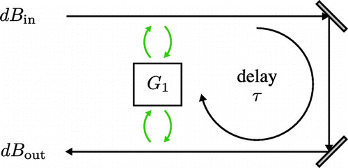
7.10.1. Approach 1: introduce fictitious SLH components

Some intuition for the first approach, due to Tabak and Mabuchi, can be gained by realizing that time delays in propagation are a special case of dispersive propagation (time delay is linear dispersion). Therefore it is likely that one can find a method to model time delays similar to the approach taken by Stace and Wiseman for approximately modeling dispersive propagation in Ref. [190] – i.e. by introducing fictitious SLH components, see Section 7.9 for details. Tabak and Mabuchi develop this intuition and provide a considerably more general solution for modeling time delays within the SLH framework [195]. They begin by considering a large SLH network with a sub-network, possibly containing multiple components and multiple input and output ports, that induces a non-negligible time delay. In the case where this sub-network only contains linear, passive elements, Tabak and Mabuchi develop a method for constructing an effective model that approximates the dynamics and input-output behavior of the original sub-network within a frequency band of interest. Notably, this effective, fictitious model is fully compatible with SLH models, i.e. localized components interconnected by zero time-delay propagating fields. The Tabak and Mabuchi approach is possible because linear, passive sub-networks can be described by a transfer function T(s), see Section 6 . The authors then approximate T(s) by a phase factor and a finite product of poles and zeros (as the number of poles and zeros increases the approximation improves). Then this resulting approximate transfer function is realized using an SLH network of cavities with different resonance frequencies and linewidths. We encourage the interested reader to look at section 4 of [195] which contains a simple example consisting of a beamsplitter and a delay. Interestingly this can be show to be equivalent to a cavity [104, section VII. B.] Two important practical issues to keep in mind when using this approach are (i) that the fictitious SLH network could have more components that the original network, and (ii) the fictitious SLH components will only provide an approximation to the time delayed dynamics, but the quality of this approximation can be improved by increasing the number of components in the fictitious network.

7.10.2. Approach 2: cascades from the past

The key insight in the approach develop by Grimsmo for incorporating time delayed propagation is that the state of the system plus field, in discrete time, can be represented using a structure similar to matrix product state (MPS) that he refers to as a super-operator product state [196] (also see the recent work by Whalen et al. [197]). With this structure Grimsmo is able to show that the propagator for a network that includes time delayed feedback can be represented as a cascade of identical systems being driven by the output field of past systems. This approach defines a propagator for the entire system, which could be used to obtain QSDEs for system or field operators. Then one can trace out the auxiliary degrees of freedom (using an appropriately generalized notion of trace) to obtain a reduced state of the time delayed system. Although Grimsmo’s approach is not integrated with the SLH framework for describing QIONs, it seems likely that such an integration is possible. In particular, the structure derived in the supplemental material of Ref. [196] is analogous to the linear fractional transformation used to derive the feedback reduction, see Rule 4 in Section 5.2. Of course, the cost to modeling time-delays in this manner is that additional fictitious components must be included in the network, as in approach 1. A numerical implementation of Grimsmo’s approach is in the development branch of QuTiP [198,199], see  [200]. As explained in Ref. [201], the long-time dynamics of QIONs with time delays can be approximated by using Grimsmo’s technique in conjunction with the “transfer tensor method” introduced Ref. [202].

Figure 14. This figure explores the three approaches (the columns), explained in this section, to modeling systems with time delay. The two example networks with delays are in the rows. The first network (row 1) is depicted in Figure 10 and represents two SLH systems with a finite delay between them and left and right propagating modes. The second network (row 2) is depicted in Figure 13 and represents an SLH note experiancing its own output feedback with a finite delay. In approach 1 (column 1) additional fictitious SLH components are introduced to model the delay. In approach 2 (column 2) the systems are driven by an cascaded version of their own outputs. If one wants to simulate the network from time zero up to some integer multipule k of the fundamental delay , then k cascades are required. The first figure in this column was adapted from [197]. In approach 3, one uses a discretized representation of the input, output and “in-loop” fields. This discrete representation is then simulated using tensor network methods.

7.10.3. Approach 3: explicit representation of the in-loop fields

Pichler and Zoller [203] use an MPS to explicitly and concisely represent the state of network components and fields. This is possible because the time bin modes in input-output theory can be related to spatial modes; recall that the field operator that interacts with the system at time t is labeled , which could equally be written as a field mode that was originally distance x from the origin, i.e. , where the propagation speed is v and . See Figure 14. Further, the Markov nature of the system-field interaction restricts the amount of entanglement that can build between components and the propagating fields and thus enables an MPS description of the system. Because the wavefunction of the entire system is evolved in this approach, one can numerically determine expectation values or correlation functions of any subsystem, the in/out fields, and even in-loop fields (field propagating between network components, which are normally eliminated under an SLH treatment). Explicitly modeling all fields enables incorporation of arbitrary propagation time delays but one should note that this approach is somewhat counter to the QION and SLH framework philosophy of simplifying the description by eliminating intermediary fields from the model. However, one could use SLH to develop models for all the components in a large network and then use the Pichler and Zoller method to directly simulate system dynamics, including delays. This approach will clearly become infeasible as the size of the network grows because although the MPS description is concise, the number of degrees of freedom becomes intractable quickly. A related approach that uses MPS to explicitly represent the system and field in real space is used by Sanchez-Burillo et al. to solve a scattering problem [204].

7.11. Software for automated modeling

The modular description of networked quantum systems enabled by the SLH framework naturally opens up the possibility of modeling large networks using automated tools. Motivated by VHDL, a hardware description language used in electronic circuit design automation, Tezak et al. have developed the Quantum Hardware Description Language (QHDL) [85], and associated design and analysis tools collected in the QNET package [205]. Like VHDL, QHDL provides a syntax and language to describe QIONs in a standardized manner. This lays the foundation for automated tools for calculating SLH triples for arbitrary QIONs described via a text file or using a graphical layout of components and interconnections. This in turn enables hierarchical modeling of large networks; once the SLH models for base components are specified, these can be interconnected in arbitrary ways and QNET will derive the SLH triple description of the resulting network. Also, SLH triples for a library of commonly used network components are predefined in QNET. Finally, there is a suite of expanding tools for analysis of these networks, including: numerical simulation of master equations resulting from SLH triples, symbolic analysis and manipulation of input-output relations associated to an SLH triple, and automated layout tools to visualize QIONs as circuits.

QHDL and QNET have been used to model and analyze complex QIONs, including optical circuits implementing quantum memories by autonomous subsystem quantum error correction [3,4], classical logic in large scale, low-power nanophotonic networks [52], and to aid analysis of a coherent, non-linear superconducting microwave experiment [38].

8. Integrated implementations of QIONs

The notion of QIONs and the SLH framework were historically developed in the context of free-space propagating fields connecting bulk optical systems, where the physical assumptions listed in Section 5.2 are generally valid. In order to build large scale QIONs one will inevitably have to turn to integrated technologies, where a huge number of components can be fabricated and networked together. Two promising integrated platforms for fabricating large-scale quantum coherent networks are silicon photonics and superconducting integrated circuits. Quantum coherent structures and high quality waveguides are routinely engineered on all of these platforms. However a number of issues arise when we consider modeling integrated coherent quantum networks on these platforms, and these make a direct application of the SLH framework to integrated systems non-trivial. In general terms, these issues are:

(1)	Integrated components can be significantly more lossy than bulk or free optical counterparts, frustrating coherent operation and quantum effects.
(2)	A localized description of interactions, captured by SLH components, may not be accurate for some integrated circuits. Examples of this are material nonlinearity and waveguide dispersion, which manifest themselves as distributed properties of a waveguide.
(3)	It remains a technical challenge to fabricate high quality integrated circulators in both silicon photonics [206] and superconducting electrical circuit technology [207], which are often very useful to many QION implementations.

Some of these issues are partially addressed by the extensions to the SLH framework discussed in Section 7, but not all. In the following, we will discuss in more detail specific issues related to porting the SLH framework to silicon photonics and superconducting circuits.

8.1. Integrated quantum coherent networks in silicon photonics

The advantages and challenges to constructing QIONs in silicon photonics are discussed in detail in Ref. [208]. We briefly summarize this discussion here, and refer the reader Ref. [208] for more details.

Integrated photonics implementations of QIONs using silicon and silicon nitride at telecommunications wavelengths are particularly interesting because of the CMOS compatibility and relative maturity of integrated photonics on these platforms. A wide variety of linear optical elements are routinely fabricated on this platform, and there is an active research effort to produce low loss nonlinear components. The primary challenges to porting the SLH framework to this platform stem from the need to capture the range of optical phenomena resulting from electromagnetic field propagation in a nonlinear, dispersive medium. The dominant physical phenomena present in silicon and silicon nitride integrated photonics at 1550 nm, and absent in bulk-optics networks are (i) dispersion, (ii) scattering by the medium, including surface roughness scattering as well as Raman and Brillouin scattering, (iii) two-photon absorption and subsequent free carrier generation and heating in the medium. In the following we discuss each of these in turn.

Dispersion needs to be taken into account both in resonant structures (e.g. cavities) and waveguides. In the former, it is largely an experimental design issue since it complicates phase matching, which subsequently makes the design of nonlinear elements such as OPOs difficult [209]. Resonant structures must be engineered to have required phase matching properties and also be resonant for frequencies of the modes participating in the desired four-wave mixing process. As long as the design of these elements accounts for dispersion, an SLH representation of these components is valid. For waveguides however, dispersion manifests itself as the dependence of the propagation velocity on the wavelength. As discussed in Section 7.9 this is incompatible with the assumptions of the SLH framework since it can invalidate the Markov approximation. Therefore, SLH modeling of QIONs implemented in integrated photonics will require engineered waveguides with minimal dispersion, that can be modeled by the perturbative approach covered in Section 7.9.

Surface roughness scattering leads to conversion of photons from modes of interest into other modes. This can be phenomenologically modeled as a linear loss mechanism that can be incorporated into the SLH description by the introduction of a fictitious beamsplitter for losses on waveguides, or the introduction of a fictitious input port with vacuum input for resonant structures. Nonlinear scattering phenomena such as Raman and Brillouin scattering are more difficult to incorporate due to the dependency of the loss coefficient on field intensity. Since the underlying scattering mechanisms ultimately arise from interactions with crystal phonons, they can be modeled fully quantum mechanically [210, Secs. 6.4.1, 11.6]. As these models show, such scattering produces incoherent loss or gain of population in the modes of interest, as well as phase decoherence. Most significantly for the SLH framework, only in some special situations can these phenomena be modeled by a coupling to a Markovian reservoir [210], which means that in most cases the effects of these nonlinear scattering processes cannot be modeled within the standard SLH framework. Accurately incorporating these nonlinear scattering processes within the SLH framework is an avenue for future work.

Aside from these nonlinear scattering processes, the dominant nonlinear optical process of concern in silicon is two-photon absorption (TPA). At the optical powers typically circulating in coherent quantum networks, this nonlinearity is too weak to invalidate the assumption of linear propagation on waveguides [208]. However, in resonant structures, e.g. ring resonator cavities, amplified field amplitudes can effectively enhance the nonlinearity. In such resonant structures the primary effect of TPA is to induce nonlinear (intensity dependent) loss. However, it also has secondary effects due to the associated creation of free carriers, whose concentration affects the refractive index of the material, which in turn changes its nonlinear and guiding properties (and causes dispersion if this change in refractive index is wavelength dependent). A natural approach to incorporating these effects within the SLH modeling framework is to apply input-output models for bulk-optical nonlinearities developed in quantum optics, e.g. Refs. [211–213], and extend these to model integrated nonlinear processes using the approach of modeling distributed transformations detailed in Section 7.7. However, this direct approach usually leads to SLH models of very large state space dimension that are difficult to simulate, and hence methods for alleviating this burden are required. Some noteworthy progress has recently been made in this direction through the formulation of a quantum model for free carrier dispersion in nanophotonic cavities [214]. This model is compatible with the SLH framework, but it is computationally difficult to directly simulate and analyze due to the large number of degrees of freedom (SLH components) that it introduces. As a result, Hamerly and Mabuchi adopt a semi-classical approximation of the dynamics to simulate and analyze their model. The approximate dynamical equations that Hamerly and Mabuchi derive from their SLH model represent a promising approach to simulation of large-scale quantum networks, and it would be fruitful to explore the full range of validity of the approximations used in Ref. [214].

8.2. SLH and superconducting microwave systems

Superconducting microwave systems are another platform that show great promise for quantum engineering [207]. Most, if not all, quantum optical components discussed in this article have excellent superconducting microwave analogs. For example, high-Q, microwave transmission line or lumped element LC resonators coupled to transmission lines have very similar internal, input, and output dynamics to optical cavities coupled to guided wave, itinerant modes [215][71, Supplementary Information]. Directional couplers and microwave hybrids act as asymmetric and symmetric optical beamsplitters, respectively. Even nonlinear optical components ranging from nonlinear crystals to single, two-level atoms may be well-approximated by superconducting microwave circuits employing nearly lossless Josephson junction elements as the fundamental nonlinearity [216].

SLH models excel at describing the dynamics of superconducting microwave systems that employ broadband, linear scattering components like directional couplers, high-Q resonant components (either linear or nonlinear), and transmission line interconnections [38,41,50,217]. In these integrated systems, as in integrated photonics, one must take care to properly model inevitable back-reflections at the interfaces between components, as well as phase delays between components. That being said, it can be easier to construct small scale, integrated superconducting microwave systems that do not suffer as much from transmission line dispersion, scattering, heating, and loss as integrated quantum photonics.

Unfortunately, SLH models are only relevant to a very particular (albeit important) subset of superconducting microwave networks. There are a number of important integrated, modular, coherent, quantum networks that are simply not expressible using IOT, let alone SLH. Essential approximations, such as the Markov approximation and the assumption that components couple via asymptotically free fields, frequently break down in microwave circuits. This is in part because microwave networks (operating at 100 MHz-100 THz frequency ranges) frequently bridge the gap between near- and far-field limits (i.e. they contain feature sizes that range from m to several cm). For example, a lumped element capacitor whose leads are connected to a transmission line is not expressible in IOT. For this circuit, one cannot approximate the interaction between the electric dipoles across the capacitor and the transmission line as narrowband (Markov approximation). This interaction occurs at all frequencies, from DC up to what ever frequency the lumped element model breaks down. Similarly, SLH is not the appropriate way to model the network of two, inductively coupled LC resonators, as these components are in each others’ near field. Increasing the physical separation between these two resonators causes the coupling strength to drop with separtation. In contrast, two LC resonators coupled to a lossless transmission line (an SLH-compatible network) each couple to the transmission line with a fixed magnitude and phase that does not vary as the distance between the two resonators varies. In this case, each entire LC resonator admits a modular description, with equations of motion for internal variables and fixed input-output relations that are constant regardless of whatever else is connected to the transmission line. However, in the case of the inductively coupled, near-field resonators, the equations of motion for each LC resonator’s variables vary with physical separation.

Thus, while SLH models can be useful for modeling a wide range of superconducting microwave quantum networks, their applicability is limited, especially in general networks that operate in the lumped element, near-field limit. Of course, the lumped element approximation of an electrical network is itself a modular modeling approach (e.g. the equation of motion for charge across and current flux through a capacitor are constant regardless of whatever else is connected to the capacitor leads). For this reason, since the 1980s, several authors have developed quite general methods for deriving the quantum dynamics of general, lumped element electrical networks [16,215,218,220], typically for superconducting microwave applications. Because these lumped element models are most applicable at a “lower level” in the hardware description of microwave networks than IOT and SLH (e.g. considering each inductor and capacitor to be separate “modules”, rather than identifying LC-resonator-type modules), such approaches tend to sacrifice modeling simplicity for accuracy. While some connections have been made over the years [16,71,216,221], there is still much work to be done to smoothly bridge between these modeling regimes. Quantum superconducting microwave circuits exist naturally in this intermediate regime, and will provide an excellent context to develop a more complete set of modeling techniques for quantum electromagnetic networks for years to come.

9. Outlook

The theory and practice of QIONs have attracted steady and growing interest over several decades, starting with the development of IOT in the 1980s, then cascaded models in the 1990s, the development of the SLH framework in the 2000s, and extensions of SLH in the 2010s. The popularity of the framework may be attributed to the conceptual clarity and computational simplifications that come from the modular approach of networking many quantum components (such as resonators, atoms or atom-like defects) via asymptotically free fields. We have attempted to summarize the development of QION up through the development of the SLH framework and some of its recent extensions. Our aim is to attract a broader audience to apply QION concepts in their own work.

While the theory of QIONs has become quite well-developed, and IOT has proven to be a perennially popular framework for analyzing quantum optical (and increasingly quantum microwave) experiments since the 1990s, fostering more experimental application of QION models to complement and guide the theoretical developments is perhaps the most pressing need for the field. Indeed, many of the extensions to SLH considered in the past decade have focused on relaxing various assumptions in the original formulation, such as dispersionless waveguides and zero time delay propagation, to better reflect experimental reality, or developing methods for including common experimental non-idealities, such as component back reflections. Similarly, the development of automated software tools like QNET for SLH modeling should also foster adoption of these techniques by the applied physics and engineering communities. Looking ahead, we identify three key areas of development for the SLH modeling framework:

(1)	Incorporation of non-Markovian coupling between localized components and propagating fields. As QION implementations migrate from free-space optics to the solid-state, as discussed in Section 8, many physical effects (e.g. weak dispersion) will manifest as a non-Markovian coupling between localized components and input-output fields. Therefore relaxing the Markov approximation will be a critical need in such scenarios. Progress in experiments has lead to renewed interest in this issue, with some recent works, by [222], Zhang et al. [223] and Gough [224]. The proposal by Zhang et al. [223] is interesting because they re-derive the cascade and concatenation product for non-Markovian systems. An SLH compatible approach is that taken by Xue et al. [225,226]. These recent studies have built on the older works by Imamoḡlu et al. [227,228], Jack et al. [99,100] and the pseudomodes approach [229,230] which represent first forays into non-Markovain input-output theory.
(2)	Development of analytic or numerical techniques or approximations for simulating the dynamics or steady-state properties of large-scale QIONs. Brute-force simulation of QION dynamics becomes intractable as the number of components in the networks becomes large. Therefore, useful approximation techniques, applied at the network level or at the level of approximating the state of the nodes of the network, are desirable to reduce the simulation burden and enable numerical analysis of large-scale QIONs. In Section 7.6 we explained one model reduction technique, namely adiabatic elimination. Some other techniques that have recently been explored are: generalized Schrieffer-Wolff transformations for dissipative systems[231], semi-classical approximation of the Wigner function description of QION dynamics [52], the kernel function approximation for nonlinear input-output models [232], a quasi-principal components approach to model reduction for nonlinear cavity degrees of freedom [233], and a method for unitary model transformation to represent systems using low dimensional manifolds  [234]. Another promising direction is to use techniques from matrix product state and tensor network literature [235,236] to represent and simulate large QIONs; recent work aimed at modeling time-delays in QIONs (covered in Section 7.10) represent initial steps in this direction. Development of such approximations and a good understanding of their regimes of applicability will be a critical need for scaling up SLH-based analysis.
(3)	The design and synthesis of nonlinear QIONs and feedback controllers. The analysis of nonlinear QIONs – with or without model reduction – is a unique strength of the SLH framework, but few tools exist within the framework for design of such networks (in contrast to linear QIONs, for which, as discussed in Section 6.3, there exist several tools for analysis, design and synthesis). One would ideally like an algorithm or tool that accepts as input equations of motion specifying the behavior of a component, and produces a realizable QION built from a library of pre-specified components that approximates this behavior; something similar in spirit to synthesizing large unitary transformations out of a universal gate set in quantum computation [1]. Design and synthesis of non-linear systems is a notoriously difficult problem, so we expect that progress on this front will be difficult. However, any such progress will have high impact since most applications on QIONs require some nonlinear behavior.

Progress in any of these directions has the potential to expand the scope and applicability of QIONs.

On a more general note, we observe that many of the near term theoretical challenges for QIONs involve blurring the boundaries between what is and what is not a QION model. The ideal ending point of this trend is analogous to the coexistence and frequent hybridization of lumped- and distributed-element component and network models in practical classical electronics. What might constitute a clear advance for QION modeling, for example, is a well-defined and easily applied method for systematically relaxing the zero time delay approximation with first, second, to nth order corrections that connect canonical SLH models to QION models where time delay is fully modeled. Recent attempts at extending the SLH framework to incorporate time delayed propagation and relax the Markov approximation represent some progress in this direction.

We hope that this review demonstrates that the QION is a concept for thinking about networked quantum systems. In addition to inherent modularity in representation this concept is compatible with many control theoretic and systems analysis tools, which we have attempted to survey. With increasing engagement from the applied physics, engineering and applied mathematics communities, we believe the maturity and applicability of the QION concept will only increase.

Acknowledgements

We gratefully acknowledge useful exchanges, on several topics, with (in alphabetical order): Ben Baragiola, Luc Bouten, Dainel Brod, Rob Cook, John Gough, Arne Grimsmo, Michael Hush, Matt James, Ekin Kocabaş, Anton Kockum, Clemens Müller, Hendra Nurdin, Ian Petersen, Daniel Soh, Tom Stace, Jason Twamley, Alkabtin Wadie, Simon Whalen, Howard Wiseman, Matt Woolley, Shibei Xue, and Guofeng Zhang. Special thanks goes to Ben and Rob for many useful suggestions, Jason and Ben for stressing the importance of adding Remark 8, and Clemens for suggesting and then correcting Remark 10.

Additional information

Funding

JC was supported in part by Perimeter Institute for Theoretical Physics and the Australian Research Council   through a Discovery Early Career Researcher Award (DE160100356); via the Centre of Excellence in Engineered Quantum Systems (EQuS), project number CE110001013. Research at Perimeter Institute is supported by the Government of Canada through the Department of Innovation, Science and Economic Development and by the Province of Ontario through the Ministry of Research, Innovation and Science. MS was supported by the Laboratory Directed Research and Development program at Sandia National Laboratories. Sandia National Laboratories is a multimission laboratory managed and operated by National Technology and Engineering Solutions of Sandia, LLC., a wholly owned subsidiary of Honeywell International, Inc., for the U.S. Department of Energy’s National Nuclear Security Administration under contract DE-NA-0003525.

Notes

No potential conflict of interest was reported by the authors.

1 We note that there are formulations of IOT for fermionic itinerant quanta [60–62], and even a unified formal treatment of bosonic and fermionic theory [63], however we will only focus on the bosonic case in this review.

2 Fundamentally this is because the integrand is independent of the increment in the Itō definition (since the increment is in the future of where the integrand is evaluated). This independence makes certain manipulations significantly easier.

3 This philosophy is motivated by electrical circuit theory where circuit component (e.g. resistor) descriptions are independent of the input signals.

4 Note that this S-matrix is distinct, but related to, the scattering matrix that forms the first element in any SLH triple. We overload this notation since the use of the symbol S has become standard in both communities, and the type of scattering matrix referred to is usually clear from context.

Appendix 1

SLH representation of some basic components

In this appendix we list SLH triples for some commonly encountered network components.

(1)	Phase shifter: A phase shifter has a single input and output field. SLH triple: (219) where is the phase shift angle.
(2)	Beam splitter: This is a system with two inputs and two outputs. If we choose the convention that the reflected fields are the output pairs to the input fields, then the SLH triple for a beam splitter is: (A1) The entries of the scattering matrix must satisfy constraints stemming from the unitarity; i.e. .
(3)	Coherent drive: This element displaces the input state in the phase plane by . SLH triple: (A2)
(4)	One-sided cavity: A perfectly reflecting mirror and a partially transparent mirror with photon decay rate . The primary quantized mode within the cavity has frequency detuning and annihilation operator a. SLH triple: (A3)
(5)	One-sided cavity with a Kerr nonlinearity: We take the previous model and add the Kerr nonlinearity to the cavity Hamiltonian (A4)
(6)	Fabry-Perot cavity: A two-sided cavity with two partially transparent mirrors. SLH triple: (A5) where are the photon decay rates of the two mirrors.
(7)	Crossed cavites (or a two mode cavity) with a cross Kerr nonlinearity: Consider two one sided cavites with frequencies that are coupled via a cross Kerr nonlinearity . The SLH parameterization for this system is (A6)
(8)	Degenerate OPO: A finite bandwith degenerate optical parametric oscillator (OPO) is modeled by a cavity model with SLH triple: (A7) where a is the cavity mode, is the cavity decay rate, and E parameterizes the OPO nonlinearity.
(9)	Two mode squeezing via a nonlinearity: with a classical and undepleted pump approximation we have the SLH triple: (A8) where is the effective pump amplitude (i.e. proportional to the nonlinearity multiplied by the pump amplitude), and is the pump frequency. By transforming to a rotating frame at half the pump frequency (i.e. we obtain (A9)
(10)	Optomechanical system with a radiation pressure coupling: a single sided optical cavity with a mechanically compliant mirror, the input field probes the cavity. SLH triple is: (A10) where is the photon decay rate of the cavity, are detunings from the carrier frequency to resonant frequencies of the cavity mode and mechanical mode, respectively, and g is the coupling between the electromagnetic and mechanical modes. The parameter is the coupling rate of the thermal phonon bath to the mechanical mode and is the occupation number of thermal phonons in the bath. Extensions of this model are discussed in detail in Refs. [237,238].
(11)	Linearized optomechanical system: Linearizing the previous model (see section 4 of Milburn and Woolley [237]), we have the SLH triple: (A11) where is the photon decay rate of the cavity, are detunings from the carrier frequency to resonant frequencies of the cavity mode and mechanical mode, respectively, and g is the coupling between the electromagnetic and mechanical modes. The parameter is the coupling rate of the thermal phonon bath to the mechanics and is the occupation number of thermal phonons in the bath. In the optomechanics literature it is common to use a series of approximations, judicious choice of the detunings, and frame changes to turn this model into cooling, heating and QND measurement interactions. Extensions of this model are discussed in detail in Refs. [237–239].
(12)	Two level atom side-coupled to waveguide: A two-level atom coupled to waveguide modes with strength and to non guided modes with strength . If the atom is perfectly coupled to the waveguide. SLH triple: (A12)
(13)	Two level atom in a harmonic potential side-coupled to waveguide: We have coupling operators associated with right moving and left moving waveguide modes as well as emmision in to nonguided modes with strength where we neglect recoil into nonguided modes. As before if the atom is perfectly coupled to the waveguide. The position and momentum operators of the center of mass motion for the atom obey . The SLH triple is (A13) where is the wave vector associated with propagation in the left or right direction, the mass of the atom is m ,and the harmonic trap frequency is in a frame rotating at the optical frequency.
(14)	Open system atom-cavity systems: A single sided cavity coupled to a two level atom.The SLH triple for the first example, the Rabi model is: (A14) where is the cavity mirror transmitivity, and are the cavity mode frequency detuning and atom transition frequency, respectively, and g is the atom-field coupling strength. In the rotating wave approximation, this model becomes the Jaynes-Cummings model, with SLH triple: (A15) The generalization to the Tavis-Cummings model is obvious (A16)
(15)	Circulators: A three port circulator has the scattering matricies (A17) If the circulator is symmetric but not perfect we have , , and [141] with complex transmission, reflection, and isolation error coefficients t, r, and b, respectively. These coefficients must obey and as the S matrix is unitary [141]. The non-idealities of the circulator are then captured by the parameters [142]: , and clearly is desirable. The four port circulator is described by the scattering matricies (A18) The coefficients must obey the conditions for the matrix to be unitary. The generalization to N ports is straight forward.

References

- M.A. Nielsen and I.L. Chuang, Quantum Computation and Quantum Information, Cambridge University Press, Cambridge, 2010.
- T.D. Ladd, F. Jelezko, R. Laflamme, Y. Nakamura, C. Monroe and J.L. O’Brien, Nature 464 (2010) p.45. doi:10.1038/nature08812
- J. Kerckhoff, H. Nurdin, D. Pavlichin and H. Mabuchi, Phys. Rev. Lett. 105(4) (2010) doi:10.1103/PhysRevLett.105.040502
- J. Kerckhoff, D.S. Pavlichin, H. Chalabi and H. Mabuchi, New J. Phys. 13 (2011) p.055022. doi:10.1088/1367-2630/13/5/055022
- D.A.B. Miller, Nat Photon 4(1) (2010) p.3. doi:10.1038/nphoton.2009.240
- D.A.B. Miller, IEEE J. Select. Topics Quantum Electron. 6(6) (2000) p.1312. doi:10.1109/2944.902184
- J. Kerckhoff, May 2011.Quantum Engineering with Quantum Optics, Ph.D. thesis, Stanford University. Available at http://minty2.stanford.edu/wp/wp-content/uploads/2011/06/JKerckhoffthesis.pdf
- J.E. Gough, Philos. T. Roy. Soc. A 370(2012) (1979) p.5241. doi:10.1098/rsta.2012.0331
- G. Zhang and M.R. James, Chin. Sci. Bull. 57(18) (2012) p.2200. doi:10.1007/s11434-012-5199-7
- M.J. Collett and C.W. Phys, Rev. A 30 (1984) p.1386. doi:10.1103/PhysRevA.30.1386
- C.W. Gardiner and M.J. Collett, Phys. Rev. A 31 (1985) p.3761. doi:10.1103/PhysRevA.31.3761
- C.W. Gardiner, Phys. Rev. Lett. 70(15) (1993) p.2269. doi:10.1103/PhysRevLett.70.2269
- H.J. Carmichael, Phys. Rev. Lett. 70(15) (1993) p.2273.
- C.W. Gardiner and A.S. Parkins, Phys. Rev. A 50 (1994) p.1792. doi:10.1103/PhysRevA.50.1792
- S. Clark, A. Peng, M. Gu and S. Parkins, Phys. Rev. Lett. 91 (2003) p.177901. Available at http://journals.aps.org/prl/abstract/10.1103/PhysRevLett.91.177901.
- B. Yurke and J.S. Denker, Phys. Rev. A 29 (1984) p.1419. doi:10.1103/PhysRevA.29.1419
- M. Kolobov and I. Sokolov, Opt. Spectroscopy 62 (1987) p.69.
- R.L. Hudson and K.R. Parthasarathy, Commun. Math. Phys. 93(3) (1984) p.301. doi:10.1007/BF01258530
- A.S. Kholevo, J. Sov. Math. 56(5) (1991) p.2609. doi:10.1007/BF01095973
- K.R. Parthasarathy, An Introduction to Quantum Stochastic Calculus, Springer Science & Business Media, Basel, 2012.
- L. Accardi, Y.G. Lu and I. Volovich, Quantum Theory and its Stochastic Limit, Springer Science & Business Media, Berlin, 2013.
- L. Bouten, R.V. Handel and M.R. James, SIAM J. Control Optim. 46(6) (2007) p.2199. doi:10.1137/060651239
- H.M. Wiseman and G.J. Milburn, Phys. Rev. A 49 (1994) p.4110. doi:10.1103/PhysRevA.49.4110
- S. Lloyd, Phys. Rev. A 62 (2000) p.022108. doi:10.1103/PhysRevA.62.022108
- M. Yanagisawa and H. Kimura, IEEE Trans. Autom. Control 48 (2003) p.2107. doi:10.1109/TAC.2003.820063
- M. Yanagisawa and H. Kimura, IEEE Trans. Autom. Control 48 (2003) p.2121. doi:10.1109/TAC.2003.820065
- J. Gough and M.R. James, IEEE Trans. Aut. Control 54 (2009) p.2530. doi:10.1109/TAC.2009.2031205
- J. Gough and M.R. James, Commun. Math. Phys. 287 (2009) p.1109. doi:10.1007/s00220-008-0698-8
- C. D’Helon and M.R. James, Phys. Rev. A 73 (2006) p.053803. doi:10.1103/PhysRevA.73.053803
- M.R. James, H.I. Nurdin and I.R. Petersen, IEEE Trans. Autom. Control 53(8) (2008) p.1787. doi:10.1109/TAC.2008.929378
- H.I. Nurdin, M.R. James and I.R. Petersen, Automatica 45(8) (2009) p.1837. doi:10.1016/j.automatica.2009.04.018
- M.R. James and J.E. Gough, IEEE Trans. Autom. Control 55(8) (2010) p.1806.
- R. Hamerly and H. Mabuchi, Phys. Rev. Lett. 109 (2012) p.173602. doi:10.1103/PhysRevLett.109.173602
- N. Yamamoto, Phys. Rev. X 4 (2014) p.041029. doi:10.1103/PhysRevX.4.041029
- H. Mabuchi, Phys. Rev. A 78 (2008) p.032323. doi:10.1103/PhysRevA.78.032323
- S. Iida, M. Yukawa, H. Yonezawa, N. Yamamoto and A. Furusawa, IEEE Trans. Automat. Contr. 57(8) (2012) p.2045. Available at http://dblp.uni-trier.de/db/journals/tac/tac57.html\#IidaYYYF12
- O. Crisafulli, N. Tezak, D.B.S. Soh, M.A. Armen and H. Mabuchi, Opt. Express 21(15) (2013) p.18371. Available at http://www.opticsexpress.org/abstract.cfm?URI=oe-21-15-18371
- J. Kerckhoff and K.W. Lehnert, Phys. Rev. Lett. 109 (2012) p.153602. doi:10.1103/PhysRevLett.109.153602
- H. Mabuchi, Appl. Phys. Lett. 99 (2011) p.153103. doi:10.1063/1.3650250
- Z. Zhou, C. Liu, Y. Fang, J. Zhou, R.T. Glasser, L. Chen, J. Jing and W. Zhang, Appl. Phys. Lett. 101 (2012) p.191113. doi:10.1063/1.4767133
- J. Kerckhoff, R.W. Andrews, H.S. Ku, W.F. Kindel, K. Cicak, R.W. Simmonds and K.W. Lehnert, Phys. Rev. X 3 (2013) p.021013. doi:10.1103/PhysRevX.3.021013
- P. Schindler, J.T. Barreiro, T. Monz, V. Nebendahl, D. Nigg, M. Chwalla, M. Hennrich and R. Blatt, Science 332(6033) (2011) p.1059. doi:10.1126/science.1203329
- M.D. Reed, L. DiCarlo, S.E. Nigg, L. Sun, L. Frunzio, S.M. Girvin and R.J. Schoelkopf, Nature 482(7385) (2012) p.382. doi:10.1038/nature10786
- M. Aspelmeyer, T.J. Kippenberg and F. Marquardt, Rev. Mod. Phys. 86 (2014) p.1391. doi:10.1103/RevModPhys.86.1391
- Y. Liu, S. Shankar, N. Ofek, M. Hatridge, A. Narla, K.M. Sliwa, L. Frunzio, R.J. Schoelkopf and M.H. Devoret, Phys. Rev. X 6 (2016) p.011022. doi:10.1103/PhysRevX.6.011022
- T. Nguyen, C.D. Hill, L.C.L. Hollenberg and M.R. James, Surface Code Continuous Quantum Error Correction using Feedback, In 2015 54th IEEE Conference on Decision and Control (CDC), Osaka, 2015, p. 7101
- C. Ahn, A.C. Doherty and A.J. Landahl, Phys. Rev. A 65 (2002) p.042301. doi:10.1103/PhysRevA.65.042301
- M. Sarovar, C. Ahn, K. Jacobs and G.J. Milburn, Phys. Rev. A 69 (2004) p.052324. doi:10.1103/PhysRevA.69.052324
- Z. Shi and H.I. Nurdin, Quantum Inform Process 14(1) (2015) p.337. doi:10.1007/s11128-014-0845-4
- F. Motzoi, E. Halperin, X. Wang, K.B. Whaley and S. Schirmer, Phys. Rev. A 94 (2016) p.032313. doi:10.1103/PhysRevA.94.032313
- H. Mabuchi, Appl. Phys. Lett. 98 (2011) p.193109. doi:10.1063/1.3589994
- C. Santori, J.S. Pelc, R.G. Beausoleil, N. Tezak, R. Hamerly and H. Mabuchi, Phys. Rev. Appl. 1 (2014) p.054005. doi:10.1103/PhysRevApplied.1.054005
- A. Frisk Kockum, P. Delsing and G. Johansson, Phys. Rev. A 90 (2014) p.013837. doi:10.1103/PhysRevA.90.013837
- M.V. Gustafsson, T. Aref, A.F. Kockum, M.K. Ekström, G. Johansson and P. Delsing, Science 346(6206) (2014) p.207. doi:10.1126/science.1257219/
- B. Fan, G. Johansson, J. Combes, G.J. Milburn and T.M. Stace, Phys. Rev. B 90 (2014) p.035132. doi:10.1103/PhysRevB.90.035132
- D.J. Brod and J. Combes, Phys. Rev. Lett. 117 (2016) p.080502. doi:10.1103/PhysRevLett.117.080502
- D.J. Brod, J. Combes and J. Gea-Banacloche, Phys. Rev. A 94 (2016) p.023833. doi:10.1103/PhysRevA.94.023833
- J.H. Shapiro, Phys. Rev. A 73 (2006) p.062305. doi:10.1103/PhysRevA.73.062305
- J. Gea-Banacloche, Phys. Rev. A 81 (2010) p.043823. doi:10.1103/PhysRevA.81.043823
- G.J. Milburn, Aust. J. Phys. 53(4) (2001) p.477. doi:10.1071/PH00003
- C. Gardiner, Opt. Commun. 243(1) (2004) p.57. doi:10.1016/j.optcom.2004.05.061
- D.B. Applebaum and R.L. Hudson, Commun. Math. Phys. 96(4) (1984) p.473. doi:10.1007/BF01212531
- R.L. Hudson and K.R. Parthasarathy, Comm. Math. Phys. 104(3) (1986) p.457. Available at http://projecteuclid.org/euclid.cmp/1104115087
- C.W. Gardiner and P. Zoller, Quantum Noise, Springer, Berlin, 2004.
- L. Accardi, I. Volovich and Y.G. Lu, Quantum Theory and its Stochastic Limit, Springer, Berlin, 2002.
- J. Gough, J. Math. Phys. 47(11) (2006) p.113509. doi:10.1063/1.2354331
- T.A. Brun, Amer. J. Phys. 70(7) (2002) p.719–737. doi:10.1119/1.1475328
- M. Yanagisawa, Phys. Rev. A 82 (2010) p.033820. doi:10.1103/PhysRevA.82.033820
- L. Bouten, R. van Handel and M.R. James, SIAM Rev. 51(2) (2009) p.239. doi:10.1137/060671504
- J.E. Gough and M.R. James, The Series Product for Gaussian Quantum Input Processes. 2016. https://arxiv.org/abs/1602.01991
- A.A. Clerk, M.H. Devoret, S.M. Girvin, F. Marquardt and R.J. Schoelkopf, Rev. Mod. Phys. 82 (2010) p.1155. doi:10.1103/RevModPhys.82.1155
- C.W. Gardiner, Handbook of Stochastic Methods, Springer, Berlin, 2004.
- C.W. Gardiner, A.S. Parkins and P. Zoller, Phys. Rev. A 46(7) (1992) p.4363. doi:10.1103/PhysRevA.46.4363
- P. Zoller and C.W. Gardiner, Quantum Noise in Quantum Optics: the Stochastic Schr odinger Equation. 2008. Available at https://arxiv.org/abs/quant-ph/9702030
- E. Wong and M. Zakai, Int. J. Eng. Sci. 3(2) (1965) p.213. doi:10.1016/0020-7225(65)90045-5
- R. van Handel, J.K. Stockton and H. Mabuchi, J. Opt. B: Q. Semiclass. Opt. 7 (2005) p.S179. doi:10.1088/1464-4266/7/10/001
- H.M. Wiseman, Quantum trajectories and feedback, Ph.D. thesis, University of Queensland, 1994. Available at http://www.ict.griffith.edu.au/wiseman/PhDThesis.ps.z
- K. Jacobs, Topics in Quantum Measurement and Quantum Noise, Ph.D. thesis, Imperial College, London, 1998. Available at https://arxiv.org/abs/quant-ph/9810015.
- R.L. Cook, Continuous Measurement and Stochastic Methods in Quantum Optical Systems, Ph.D. thesis, The University of New Mexico, 2013. Available at https://arxiv.org/abs/1301.6193.
- A.S. Holevo, Proc. Roy. Soc. Edinbur: Sect A Math. 126 2(1996), p. 375. doi:10.1017/S0308210500022794
- A.S. Holevo, Quantum Prob. Commun. XI (2003), p. 199
- J.E. Gough, R. Gohm and M. Yanagisawa, Phys. Rev. A 78 (2008) p.062104. doi:10.1103/PhysRevA.78.062104
- L. Bouten, J. Stockton, G. Sarma and H. Mabuchi, Phys. Rev. A 75 (2007) p.052111. doi:10.1103/PhysRevA.75.052111
- J. Kerckhoff, L. Bouten, A. Silberfarb and H. Mabuchi, Phys. Rev. A 79 (2009) p.024305. doi:10.1103/PhysRevA.79.024305
- N. Tezak, A. Niederberger, D.S. Pavlichin, G. Sarma and H. Mabuchi, Philos. Trans. Roy. Soc. A: Math. Phys. Eng. Sci. 370(1979) (2012) p.5270. doi:10.1098/rsta.2011.0526
- A. Barchielli, J. Phys. A: Math. Gen. 20(18) (1999) p.6341. doi:10.1088/0305-4470/20/18/034
- J. Gough, Phys. Rev. E 90(6) (2014) p.062109. doi:10.1103/PhysRevE.90.062109
- H.J. Carmichael, An Open Systems Approach to Quantum Optics, In Lecture Notes in Physics Monographs, Vol. 18, Springer-Verlag, Berlin Heidelberg, 1993, lectures Presented at the Université Libre de Bruxelles, October 28 to November 4, 1991
- H.M. Wiseman and G.J. Milburn, Quantum Measurement and Control, Cambridge University Press, 2010. Available at https://books.google.com/books?id=ZNjvHaH8qA4C.
- K. Jacobs and D.A. Steck, Contemp. Phys. 47(5) (2006) p.279. doi:10.1080/00107510601101934
- A. Barchielli, L. Lanz, and G.M. Prosperi, Il Nuovo Cimento B (1971--1996). 72 1(1982), p. 79. doi:10.1007/BF02894935
- A. Barchielli, Phys. Rev. A 34 (1986) p.1642. doi:10.1103/PhysRevA.34.1642
- C.M. Caves and G.J. Milburn, Phys. Rev. A 36 (1987) p.5543. doi:10.1103/PhysRevA.36.5543
- V.P. Belavkin, Nondemolition Measurements, Nonlinear Filtering and Dynamic Programming of Quantum Stochastic Processes, In A. Blaquiére (Ed.), Proceedings of the Bellman Continuum Workshop 1988, Jun 13–14, Springer, Berlin, 1989, p. 245. doi:10.1007/BFb0041197. Sophia Antipolis, France, Modeling and Control of Systems: in Engineering, Quantum Mechanics, Economics and Biosciences,
- J. Dalibard, Y. Castin and K. Mølmer, Phys. Rev. Lett. 68 (1992) p.580. doi:10.1103/PhysRevLett.68.580
- P. Goetsch and R. Graham, Phys. Rev. A 50 (1994) p.5242. doi:10.1103/PhysRevA.50.5242
- H.M. Wiseman, J. Opt. B: Qantum Semiclass. Opt. 8(1) (1996) p.205. doi:10.1088/1355-5111/8/1/015
- A. Barchielli, and A.M. Paganoni, Quantum Semiclassical Opt.: J. Eur. Opt. Soc. Part B. 8 1(1990), doi:10.1088/1355-5111/8/1/011
- M.W. Jack and M.J. Collett, D. F. Walls: Phys. Rev. A 59 (1999) p.2306. doi:10.1103/PhysRevA.59.2306
- M.W. Jack and M.J. Collett, Phys. Rev. A 61 (2000) p.062106. doi:10.1103/PhysRevA.61.062106
- R. Simon, N. Mukunda, and B. Dutta, Phys. Rev. A. 49 (1994), p. 1567. Available at http://journals.aps.org/pra/abstract/10.1103/PhysRevA.49.1567.
- J.E. Gough, R. Gohm, and M. Yanagisawa, Phys. Rev. A. 78 6(2008), p. 062104. Available at http://pra.aps.org/abstract/PRA/v78/i6/e062104.
- R.F. Stengel, Optimal Control and Estimation, Dover Publications, New York, 1994,
- J.E. Gough, M.R. James and H.I. Nurdin, Phys. Rev. A 81(2) (2010) p.023804. doi:10.1103/PhysRevA.81.023804
- C. Weedbrook, S. Pirandola, R. García-Patrón, N.J. Cerf, T.C. Ralph, J.H. Shapiro, and S. Lloyd, Rev. Mod. Phys.. 84 2(2012), p. 621. Available at http://rmp.aps.org/abstract/RMP/v84/i2/p6211.
- J.E. Gough, and S. Wildfeuer, Phys. Rev. A. 80 4(2009), p. 042107. Available at http://journals.aps.org/pra/abstract/10.1103/PhysRevA.80.042107.
- I.R. Petersen, Quantum Linear Systems Theory. 2016. http://arxiv.org/abs/1603.04950v1.
- J.E. Gough and G. Zhang, Automatica 59 (2015) p.139. doi:10.1016/j.automatica.2015.06.023
- H.I. Nurdin, M.R. James and A.C. Doherty, SIAM J. Control Optim. 48(4) (2009) p.2686. doi:10.1137/080728652
- H.I. Nurdin, IEEE Trans. Autom. Control. 55 4(2010), p. 1008. Available at http://ieeexplore.ieee.org/xpls/absall.jsp?arnumber=5404766.
- H.I. Nurdin, IEEE Trans. Autom. Control. 55 10(2010), p. 2439. Available at http://ieeexplore.ieee.org/xpls/absall.jsp?arnumber=5535129.
- H.I. Nurdin, S. Grivopoulos and I.R. Petersen, Automatica 69 (2016) p.324. doi:10.1016/j.automatica.2016.03.002
- H.I. Nurdin, IEEE Trans. Autom. Control. 59 9(2014), p. 2413. Available at http://ieeexplore.ieee.org/xpl/articleDetails.jsp?reload=truearnumber=6812167.
- O. Techakesari and H.I. Nurdin, Syst. Control Lett. 78 (2015) p.25. doi:10.1016/j.sysconle.2015.01.010
- M. Guta, and N. Yamamoto, IEEE Trans. Autom. Control. 61 4(2016), p. 921. Available at http://ieeexplore.ieee.org/xpls/absall.jsp?arnumber=7130587.
- K.J. Blow, R. Loudon, and S.J.D. Phoenix, T.J. Shepherd, Phys. Rev. A. 42 (1990), p. 4102. Available at https://dx.doi.org/10.1103/PhysRevA.42.4102.
- B.R. Mollow, Phys. Rev. A 12 (1975) p.1919. doi:10.1103/PhysRevA.12.1919
- J.E. Gough, M.R. James, and H.I. Nurdin, J. Combes, Phys. Rev. A. 86 (2012), p. 043819. doi:10.1103/PhysRevA.86.043819
- J.E. Gough, and G. Zhang, EPJ Quantum Tech. 2. doi:10.1140/epjqt/s40507-015-0027-z
- P.D. Drummond, and M.D. Reid, Phys. Rev. A. 37 (1988), p. 1806. Available at https://dx.doi.org/10.1103/PhysRevA.37.1806.
- B.Q. Baragiola, and R.L. Cook, J. Combes, Phys. Rev. A. 86 p. 013811. Available at https://dx.doi.org/10.1103/PhysRevA.86.013811.
- A.S. Parkins and C.W. Gardiner, Phys. Rev. A 37 (1988) p.3867. doi:10.1103/PhysRevA.37.3867
- H. Ritsch and P. Zoller, Phys. Rev. A 38 (1988) p.4657. doi:10.1103/PhysRevA.38.4657
- H. Ritsch and P. Zoller, Phys. Rev. Lett. 61 (1988) p.1097. doi:10.1103/PhysRevLett.61.1097
- M.D. Reid and D.F. Walls, Phys. Rev. A 34 (1986) p.4929. doi:10.1103/PhysRevA.34.4929
- X.B. Wang, T. Hiroshima, A. Tomita, and M. Hayashi, Phys. Rep. 448 (2007), p. 1. Available at http://www.sciencedirect.com/science/article/pii/S0370157307001822.
- R. Loudon, The Quantum Theory of Light, 3rd ed., OUP Oxford, New York, 2000.
- K.M. Gheri, K. Ellinger, T. Pellizzari and P. Zoller, Fortschritte der Physik 46(4–5) (1998) p.401. doi:10.1002/(SICI)1521-3978(199806)46:4/5401::AID-PROP4013.0.CO;2-W
- J.E. Gough, M.R. James, and H.I. Nurdin, New J. Phys. 16 (2014), p. 075008. Available at http://iopscience.iop.org/article/10.1088/1367-2630/16/7/075008/meta.
- B.Q. Baragiola and J. Combes, Quantum Trajectories for Propagating Fock States, 2017. Available at https://arxiv.org/abs/1704.00101
- H. Song, G. Zhang and Z. Xi, SIAM J. Control Optim. 54(3) (2016) p.1602. doi:10.1137/15M1023099
- J.E. Gough, M.R. James and H.I. Nurdin, Quantum Inform Process 12(3) (2013) p.1469. doi:10.1007/s11128-012-0373-z
- B.Q. Baragiola, Open Systems Dynamics for Propagating Quantum Fields, Ph.D. thesis, University of New Mexico. (2014). Available at https://arxiv.org/abs/1408.4447.
- A. Ferraro, S. Olivares, and M.G.A. Paris, Gaussian States in Continuous Variable Quantum Information, 2005. https://arxiv.org/abs/quant-ph/0503237.
- C.M. Caves and B.L. Schumaker, Phys. Rev. A 31 (1985) p.3068. doi:10.1103/PhysRevA.31.3068
- C.W. Gardiner, Phys. Rev. Lett. 56 (1986) p.1917. doi:10.1103/PhysRevLett.56.1917
- J.I. Cirac, Phys. Rev. A 46 (1992) p.4354. doi:10.1103/PhysRevA.46.4354
- R. Dum, A.S. Parkins, P. Zoller and C.W. Phys, Rev. A 46 (1992) p.4382. doi:10.1103/PhysRevA.46.4382
- Q.A. Turchette, N.P. Georgiades, C.J. Hood, H.J. Kimble and A.S. Parkins, Phys. Rev. A 58 (1998) p.4056. doi:10.1103/PhysRevA.58.4056
- K.W. Murch, S.J. Weber, K.M. Beck, E. Ginossar and I. Siddiqi, Nature 499(7456) (2013) p.62. doi:10.1038/nature12264
- S. Hagelin, IEEE Trans Microw Theory Tech 17(6) (1969) p.328.
- Y. Ayasli, IEEE Trans. Microw. Theory Tech. 28(3) (1980) p.200. doi:10.1109/TMTT.1980.1130041
- S.J.M. Habraken, K. Stannigel, M.D. Lukin, P. Zoller, and P. Rabl, New J. Phys.. 14 11(2012), p. 115004. Available at http://stacks.iop.org/1367-2630/14/i=11/a=115004
- J. Kerckhoff, K. Lalumière, B.J. Chapman, A. Blais and K.W. Lehnert, Phys. Rev. Appl. 4 (2015) p.034002. doi:10.1103/PhysRevApplied.4.034002
- L. Ranzani and J. Aumentado, New J. Phys. 17(2) (2015) p.023024. doi:10.1088/1367-2630/17/2/023024
- F. Lecocq, L. Ranzani, G.A. Peterson, K. Cicak, R.W. Simmonds, J.D. Teufel and J. Aumentado, Phys. Rev. Applied 7 (2017) p.024028. doi:10.1103/PhysRevApplied.7.024028
- P. Lodahl, S. Mahmoodian, and S. Stobbe, Chiral Quantum Opt., 2016. http://arxiv.org/abs/1608.00446
- K. Lalumière, B.C. Sanders, A.F. van Loo, A. Fedorov, A. Wallraff and A. Blais, Phys. Rev. A 88 (2013) p.043806. doi:10.1103/PhysRevA.88.043806
- A.F. van Loo, A. Fedorov, K. Lalumière, B.C. Sanders, A. Blais and A. Wallraff, Science 342(6165) (2013) p.1494. doi:10.1126/science.1244324
- T. Caneva, M.T. Manzoni, T. Shi, J.S. Douglas, J.I. Cirac, D.E. Chang, New J. Phys. 17 11(2015), p. 113001. Available at http://stacks.iop.org/1367-2630/17/i=11/a=113001
- G. Calajó, F. Ciccarello, D. Chang and P. Rabl, Phys. Rev. A 93 (2016) p.033833. doi:10.1103/PhysRevA.93.033833
- J.D. Hood, A. Goban, A. Asenjo-Garcia, M. Lu, S.-P. Yu, D.E. Chang and H.J. Kimble, Proc. Natl. Acad. Sci. 113(38) (2016) p.10507. doi:10.1073/pnas.1603788113
- A. Asenjo-Garcia, J.D. Hood, D.E. Chang and H.J. Kimble, Phys. Rev. A 95 (2017) p.033818. doi:10.1103/PhysRevA.95.033818
- C.W. Gardiner, Phys. Rev. A 29 (1984) p.2814. doi:10.1103/PhysRevA.29.2814
- C.W. Gardiner and M.L. Steyn-Ross, Phys. Rev. A 29 (1984) p.2823. doi:10.1103/PhysRevA.29.2823
- M.L. Steyn-Ross and C.W. Gardiner, Phys. Rev. A 29 (1984) p.2834. doi:10.1103/PhysRevA.29.2834
- C.Cohen-Tannoudji, J.Dupont-Roc and G.Grynberg, In Atom-photon interactions: Basic Process and Appilcations, Wiley, New York, 1998.
- L. Bouten and A. Silberfarb, Commun. Math. Phys. 283(2) (2008) p.491. doi:10.1007/s00220-008-0513-6
- L. Bouten, R. van Handel and A. Silberfarb, J. Funct. Anal. 254(12) (2008) p.3123. doi:10.1016/j.jfa.2008.02.013
- P. Warszawski and H.M. Wiseman, Phys. Rev. A 63 (2000) p.013803. doi:10.1103/PhysRevA.63.013803
- J.E. Gough, H.I. Nurdin, and S. Wildfeuer, J. Math. Phys. 51(12) (2010). p.123518. doi:10.1063/1.3520513
- H.I. Nurdin, and J.E. Gough, Philos.T. Roy. Soc. A. 370 1979(2912), p. 5422. doi:10.1098/rsta.2011.0523
- M. Devoret, B. Huard, L.F. Cugliandolo, and R.J. Schoelkopf, (Eds.)Quantum Machines: Measurement Control of Engineered Quantum Systems: Lecture Notes of the Les Houches Summer School, Vol. 96, Oxford University Press, 2014,
- H. Mabuchi, Phys. Rev. A 80 (2009) p.045802. doi:10.1103/PhysRevA.80.045802
- H. Mabuchi, Qubit limit of cavity nonlinear optics: Phys. Rev. A 85 (2012) p.015806. doi:10.1103/PhysRevA.85.015806
- F. Reiter and A.S. Sørensen, Phys. Rev. A 85 (2012) p.032111. doi:10.1103/PhysRevA.85.032111
- P.D. Drummond, Phys. Rev. A 42 (1990) p.6845. doi:10.1103/PhysRevA.42.6845
- R.J. Glauber and M. Lewenstein, Phys. Rev. A 43 (1991) p.467. doi:10.1103/PhysRevA.43.467
- B. Huttner and S.M. Barnett, Phys. Rev. A 46 (1992) p.4306. doi:10.1103/PhysRevA.46.4306
- P.D. Drummond and M. Hillery, Phys. Rev. A 59 (1999) p.691. doi:10.1103/PhysRevA.59.691
- M. Liscidini, L.G. Helt and J.E. Sipe, Phys. Rev. A 85 (2012) p.013833. doi:10.1103/PhysRevA.85.013833
- F. Graffitti, D. Kundys, D.T. Reid, A.M. Brańczyk, and A. Fedrizzi, Pure Down-conversion Photons Through Sub-coherence Length Domain Engineering, 2017. https://arxiv.org/abs/1704.03683.
- C.M. Caves and D.D. Crouch, J. Opt. Soc. Am. B 4(10) (1987) p.1535. doi:10.1364/JOSAB.4.001535
- M.R. Hush, A.R.R. Carvalho, M. Hedges, and M.R. James, New J. Phys.. 15 8(2013), p. 085020. Available at http://stacks.iop.org/1367-2630/15/i=8/a=085020
- R.N. Stevenson, M.R. Hush, A.R.R. Carvalho, S.E. Beavan, M.J. Sellars, and J.J. Hope, New J. Phys.. 16 3(2014), p. 033042. Available at http://stacks.iop.org/1367-2630/16/i=3/a=033042
- S. Fu, A.R.R. Carvalho, M.R. Hush and M.R. James, Phys. Rev. A 93 (2016) p.023809. doi:10.1103/PhysRevA.93.023809
- B.J. Dalton, S.M. Barnett and P.L. Knight, J. Mod. Optic. 46(7) (1999) p.1107. doi:10.1080/09500349908230404
- S. Fan, Ş.E. Kocabaş and J.-T. Shen, Phys. Rev. A 82 (2010) p.063821. doi:10.1103/PhysRevA.82.063821
- D. Roy, C.M. Wilson, and O. Firstenberg, Strongly Interacting Photons in One-dimensional Continuum, 2016. http://arxiv.org/abs/1603.06590.
- Ş.E. Kocabaş, E. Rephaeli and S. Fan, Phys. Rev. A 85 (2012) p.023817. doi:10.1103/PhysRevA.85.023817
- S. Xu and S. Fan, Phys. Rev. A 91(4) (2015) p.043845.
- Y. Pan, D. Dong, and G. Zhang, New J. Phys. 18 3(2016), p. 033004. Available at http://stacks.iop.org/1367-2630/18/i=3/a=033004
- T. Shi, D.E. Chang, and J.I. Cirac, Phys. Rev. A. 92 (2015), p. 053834. Available at http://link.aps.org/doi/10.1103/PhysRevA.92.053834
- \c{S}.E. Kocabaş, Phys. Rev. A. 93 (2016), doi:10.1103/PhysRevA.93.033829
- A.C. Turner, C. Manolatou, B.S. Schmidt, M. Lipson, M.A. Foster, J.E. Sharping and A.L. Gaeta, Opt. Expr. 14(10) (2006) p.4357. doi:10.1364/OE.14.004357
- L. Zhang, Y. Yue, Y. Xiao-Li, J. Wang, R.G. Beausoleil and A.E. Willner, Opt. Expr. 18(12) (2010) p.13187. doi:10.1364/OE.18.013187
- L. Zhang, Q. Lin, Y. Yue, Y. Yan, R.G. Beausoleil and A.E. Willner, Opt. Express 20(2) (2012) p.1685. doi:10.1364/OE.20.001685
- T.M. Stace, H.W. Barnes, and G.J. Milburn, Phys. Rev. Lett.. 93 (2004), p. 126804. Available at http://journals.aps.org/prl/abstract/10.1103/PhysRevLett.93.126804
- T.M. Stace, Quantum Information Transfer in Solid State Devices, Ph.D. thesis, University of Cambridge, 2004.
- T.M. Stace and H.M. Wiseman, Phys. Rev. A 73(1) (2006) p.012317. doi:10.1103/PhysRevA.73.012317
- D. Kielpinski, J.F. Corney and H.M. Wiseman, Phys. Rev. Lett. 106 (2011) p.130501. doi:10.1103/PhysRevLett.106.130501
- U. Dorner and P. Zoller, Phys. Rev. A 66 (2002) p.023816. doi:10.1103/PhysRevA.66.023816
- N. Német and S. Parkins, Phys. Rev. A 94 (2016) p.023809. doi:10.1103/PhysRevA.94.023809
- M. Kraft, S.M. Hein, J. Lehnert, E. Schöll, S. Hughes and A. Knorr, Phys. Rev. A 94 (2016) p.023806. doi:10.1103/PhysRevA.94.023806
- G. Tabak, and H. Mabuchi, EPJ Quantum Tech. 3. doi:10.1140/epjqt/s40507-016-0041-9
- A.L. Grimsmo, Phys. Rev. Lett. 115(6) (2015) p.060402. doi:10.1103/PhysRevLett.115.060402
- S.J. Whalen, A.L. Grimsmo and H.J. Carmichael, Open Quantum Systems with Delayed Coherent Feedback, 2016. https://arxiv.org/abs/1702.05776.
- J. Johansson, P. Nation and F. Nori, Comput. Phys. Commun. 184(4) (2013) p.1234. doi:10.1016/j.cpc.2012.11.019
- QuTiP development team, Qutip: Quantum toolbox in python. (2016). Available at https://github.com/qutip/qutip.
- A.L. Grimsmo, Delayed feedback. (2016), Available at https://github.com/qutip/qutip-notebooks/blob/master/examples/example-nonmarkov-coherent-feedback.ipynb.
- A.L. Grimsmo, Transfer tensor method2016. Available at https://github.com/qutip/qutip-notebooks/blob/master/examples/example-nonmarkov-transfer-tensor-method.ipynb.
- J. Cerrillo and J. Cao, Phys. Rev. Lett. 112 (2014) p.110401. doi:10.1103/PhysRevLett.112.110401
- H. Pichler and P. Zoller, Phys. Rev. Lett. 116(9) (2016) p.093601. doi:10.1103/PhysRevLett.116.093601
- E. Sanchez-Burillo, D. Zueco, J.J. Garcia-Ripoll and L. Martin-Moreno, Phys. Rev. Lett. 113 (2014) p.263604. doi:10.1103/PhysRevLett.113.263604
- The QNET Package, 2016. Available at http://mabuchilab.github.io/QNET/.
- D. Jalas, A. Petrov, M. Eich, W. Freude, S. Fan, Z. Yu, R. Baets, M. Popovic, A. Melloni, J.D. Joannopoulos, M. Vanwolleghem, C.R. Doerr and H. Renner, Nat. Photon 7(8) (2013) p.579. doi:10.1038/nphoton.2013.185
- M.H. Devoret and R.J. Schoelkopf, Science 339(6124) (2013) p.1169. doi:10.1126/science.1231930
- M. Sarovar, D.B.S. Soh, J. Cox, C. Brif, C.T. DeRose, R. Camacho and P. Davids, Silicon Nanophotonics for Scalable QuantumCoherent Feedback Networks, https://arxiv.org/abs/1608.06962.
- A. Dutt, K. Luke, S. Manipatruni, A.L. Gaeta, P. Nussenzveig and M. Lipson, Phys. Rev. Appl. 3 (2015) p.044005. doi:10.1103/PhysRevApplied.3.044005
- P.D. Drummond and M. Hillery, The Quantum Theory Of Nonlinear Optics, Cambridge University Press, Cambridge, 2014.
- M.J. Collett and D.F. Walls, Phys. Rev. A 32 (1985) p.2887. doi:10.1103/PhysRevA.32.2887
- M.J. Collett and R.B. Levien, Phys. Rev. A 43 (1991) p.5068. doi:10.1103/PhysRevA.43.5068
- R.B. Levien, M.J. Collett and D.F. Walls, Phys. Rev. A 47 (1993) p.2324. doi:10.1103/PhysRevA.47.2324
- R. Hamerly and H. Mabuchi, Phys. Rev. A 92 (2015) p.023819. doi:10.1103/PhysRevA.92.023819
- M.H. Devoret, Ch. Quantum Fluctuations in Electrical Circuits., In Les Houches Session LXIII, North Holland, 1997,
- A. Blais, R.-S. Huang, A. Wallraff, S.M. Girvin and R.J. Schoelkopf, Phys. Rev. A 69 (2004) p.062320. doi:10.1103/PhysRevA.69.062320
- F. Motzoi, K.B. Whaley and M. Sarovar, Phys. Rev. A 92 (2015) p.032308. doi:10.1103/PhysRevA.92.032308
- G. Burkard, R.H. Koch and D.P. DiVincenzo, Phys. Rev. B 69 (2004) p.064503. doi:10.1103/PhysRevB.69.064503
- G. Wendin, and V. Shumeiko, Superconducting Quantum Circuits, Qubits and Computing, 2005. https://arxiv.org/abs/cond-mat/0508729.
- F. Solgun, and D.P. DiVincenzo, Multiport Impedance Quantization, 2015. https://arxiv.org/abs/1505.04116.
- S.E. Nigg, H. Paik, B. Vlastakis, G. Kirchmair, S. Shankar, L. Frunzio, M.H. Devoret, R.J. Schoelkopf and S.M. Girvin, Phys. Rev. Lett. 108 (2012) p.240502. doi:10.1103/PhysRevLett.108.240502
- L. Diósi, Phys. Rev. A 85 (2012) p.034101. doi:10.1103/PhysRevA.85.034101
- J. Zhang, Y.-X. Liu, R.-B. Wu, K. Jacobs and F. Nori, Phys. Rev. A 87 (2013) p.032117. doi:10.1103/PhysRevA.87.032117
- J. Gough, Non-Markovian Quantum Feedback Networks I: Quantum Transmission Lines, Lossless Bounded Real Property and Limit Markovian Channels, 2016. https://arxiv.org/abs/1604.02279v1
- S. Xue, M.R. Hush, and I.R. Petersen, IEEE Trans. Contr. Syst. Tech. 99 (2016) p.1. doi:10.1109/TCST.2016.2614834
- S. Xue, T. Nguyen, M.R. James, A. Shabani, V. Ugrinovskii, and R. Petersen, Modelling and Filtering for Non-markovian QuantumSystems, 2017. https://arxiv.org/abs/1704.00986.
- A. Imamo\={g}lu, Phys. Rev. A 50 (1994) p.3650. doi:10.1103/PhysRevA.50.3650
- P. Stenius and A. Imamoglu, Quantum Semicl. Opt. 8(1) (1996) p.283. doi:10.1088/1355-5111/8/1/021
- B.J. Dalton, S.M. Barnett and B.M. Garraway, Phys. Rev. A 64 (2001) p.053813. doi:10.1103/PhysRevA.64.053813
- L. Mazzola, S. Maniscalco, J. Piilo, K.-A. Suominen and B.M. Garraway, Phys. Rev. A 80 (2009) p.012104. doi:10.1103/PhysRevA.80.012104
- E.M. Kessler, Phys. Rev. A 86 (2012) p.012126. doi:10.1103/PhysRevA.86.012126
- J. Zhang, Y.X. Liu, R.B. Wu, K. Jacobs, S.K. Ozdemir, L. Yang, T.-J. Tarn, F. Nori, Nonlinear Quantum Input-output Analysis using Volterra Series. 2014. http://arxiv.org/abs/1407.8108. [quant-ph]..
- Z. Shi and H.I. Nurdin, J. Phys. D: Appl. Phys. 49(46) (2016) p.465501. doi:10.1088/0022-3727/49/46/465501
- N. Tezak, N.H. Amini, and H. Mabuchi, J. Phys. A: Math. Theor 50 (2017) p.223001. doi:10.1088/1751-8121/aa6dc3.
- J.C. Bridgeman, and C.T. Chubb, Hand-waving and Interpretive Dance: An Introductory Course on Tensor Networks. 2016. http://arxiv.org/abs/1603.03039.
- R. Orús, Annal. Phys. 349 (2014) p.117. doi:10.1016/j.aop.2014.06.013
- G.J. Milburn and M.J. Woolley, Acta Phys. Slov. 61(5) (2011) p.483. doi:10.2478/v10155-011-0005-7
- W.P. Bowen and G.J. Milburn, Quantum Optomechanics, CRC Press, Boca Raton, 2015.
- S. Ma, I.R. Petersen and M.J. Woolley, Syst. Contr. Lett. 99 (2017) p.64. doi:10.1016/j.sysconle.2016.11.013