Synergy of physics-based reasoning and machine learning in biomedical applications: towards unlimited deep learning with limited data

ABSTRACT

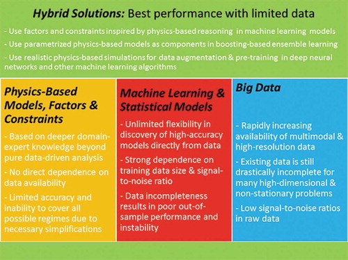
Technological advancements enable collecting vast data, i.e., Big Data, in science and industry including biomedical field. Increased computational power allows expedient analysis of collected data using statistical and machine-learning approaches. Historical data incompleteness problem and curse of dimensionality diminish practical value of pure data-driven approaches, especially in biomedicine. Advancements in deep learning (DL) frameworks based on deep neural networks (DNN) improved accuracy in image recognition, natural language processing, and other applications yet severe data limitations and/or absence of transfer-learning-relevant problems drastically reduce advantages of DNN-based DL. Our earlier works demonstrate that hierarchical data representation can be alternatively implemented without NN, using boosting-like algorithms for utilization of existing domain knowledge, tolerating significant data incompleteness, and boosting accuracy of low-complexity models within the classifier ensemble, as illustrated in physiological-data analysis. Beyond obvious use in initial-factor selection, existing simplified models are effectively employed for generation of realistic synthetic data for later DNN pre-training. We review existing machine learning approaches, focusing on limitations caused by training-data incompleteness. We outline our hybrid framework that leverages existing domain-expert models/knowledge, boosting-like model combination, DNN-based DL and other machine learning algorithms for drastic reduction of training-data requirements. Applying this framework is illustrated in context of analyzing physiological data.

GRAPHICAL ABSTRACT

KEYWORDS:

• Nonlinear dynamics
• boosting
• deep learning (DL)
• complex biomedical systems
• hybrid machine learning
• physiological state quantification

I. Introduction

Modern technological advancements made possible the collection of vast amount of data, often called Big Data, in many areas of science and industry including biomedical field [1–4]. A dramatic increase in computational power, including massively parallel computation and data retrieval using multi-core CPU and GPU units (see www.nvidia.com), creates the possibility of analyzing collected data in reasonable time using modern statistical and machine learning (ML) approaches [3,5–8]. However, the ‘Big Data’ term could be misleading in many important applications. While the amount of collected data rapidly increases with technological progress, the high dimensionality and the multi-regime nature of many problems still work against any resolution of long-standing problems of data incompleteness and curse of dimensionality that diminish the practical value of pure data-driven approaches [9–11]. In the biomedicine context, these challenges include the very high dimensionality of typical bioinformatics and medical imaging problems, the multi-regime nature and inter-personal diversity of physiological dynamics as well as the serious data limitations in personalized medicine and in detection/treatment of rare or complex abnormalities [11–14].

Increasing availability of multi-scale and multi-channel physiological data opens new horizons for quantitative modeling and applications in decision-support systems. However, practical limitations of existing approaches include both (1) the low accuracy of the simplified analytical models and simplified empirical expert-defined rules and (2) the insufficient interpretability and insufficient stability of the pure data-driven models [11–14]. Such challenges are typical for automated diagnostics from multi-channel, temporal, physiological information available in modern clinical settings. In addition, the increasing number of portable and wearable systems for collection of physiological data outside medical facilities provide an opportunity for ‘express’ and ‘remote’ diagnostics as well as early detection of irregular and transient patterns caused by developing abnormalities or subtle initial effects of new treatments. However, quantitative modeling in such applications is even more challenging due to obvious limitations on the number of data channels, the increased noise, and the non-stationary nature of considered tasks.

Methods from nonlinear dynamics (NLD), including NLD-inspired complexity measures, are natural modeling tools for adaptive biological systems with multiple feedback loops and are capable of inferring essential dynamic properties from just one, or a small number of, data channels [15–17]. However, most NLD indicators require large record lengths from long durations of data acquisition to achieve calculation stability, which significantly limits their practical value [11–17]. Many of these challenges in biomedical modeling could be overcome by techniques of boosting and similar ensemble learning that are capable of discovering robust multi-component meta-models by employing existing simplified models and other incomplete empirical knowledge [10,18,19]. We have previously proposed such leveraging of physics-based reasoning (formalized as NLD-inspired complexity measures) and boosting as well as demonstrated potential benefits of this approach in express diagnostics and early detection of treatment responses from short beat-to-beat heart rate (RR) time series [11–14] and gait data [20].

Recent advancements in deep learning (DL) frameworks based on deep neural networks (DNN) drastically improved the accuracy of data-driven approaches in image recognition, natural language processing, and other applications. The key advantage of DL is its systematic approach for the independent training of groups of DNN layers, including unsupervised training of auto-encoders for the hierarchical representation of raw input data (i.e. automatic feature selection and dimensionality reduction) and the supervised re-training of several final layers in the transfer learning that compensate for data incompleteness. However, severe data limitations and/or absence of relevant problem for transfer learning can drastically reduce the advantages of DNN-based DL. For example, pure data-driven auto-encoders dealing with high-dimensional input data require a large amount of data for effective operation [21–23].

Domain-expert models/rules obtained by a deeper understanding of the considered application scope could play a key role in cases with severe incompleteness of training data because of natural dimensionality reduction and usage of domain-specific constraints [10–14,23]. However, such simplified models are often biased and not capable to cover all possible regimes. On the other hand, comprehensive incorporation of this domain knowledge into standard DNN-based DL is problematic, except for straightforward guidance in factor selection [23].

However, alternative machine learning algorithms, such as different flavors of boosting, combine key advantages of DNNs such as hierarchical data representations and iterative component-wise learning with operational simplicity and the ability of direct incorporation of domain-expert knowledge [10–14,18,19]. Also, the performance of boosting-based models is often comparable to that of DNN [24,25]. Similarly, existing simplified models can be used for the generation of a large amount of realistic synthetic data that can be effectively used for DNN pre-training. Finally, recently we have shown that the techniques of boosting and DNN can be effectively combined within hybrid frameworks that allow the incorporation of existing domain-expert knowledge [23]. Thus, in this review, we refer to DL paradigm not only in the context of DNN-based implementation but in the wider scope.

Here, we start with a short review of existing machine learning approaches, focusing on their limitations due to training-data incompleteness. Then, we outline a hybrid framework that leverages the existing domain-expert knowledge, boosting, DNN-based DL, and other machine learning algorithms to achieve drastic alleviation of training-data requirements. Finally, the application of this framework to the analysis of physiological and other biomedical data analysis is discussed and illustrated.

II. Modern machine learning: advantages and limitations

1. Big data and limitation of standard statistical frameworks

The ongoing digital revolution has provided a relatively inexpensive means to collect and store multi-scale, multi-channel, physiological data. Modern hospitals and research centers are well-equipped with high-resolution monitoring, diagnostic, and other data-collection devices. Moreover, many portable systems for real-time collection and display of physiological data have become affordable for individual use outside of specialized medical facilities. These include Holter monitors and similar devices for electrocardiogram (ECG) and heart-rate recording and specialized systems for electroencephalogram (EEG), electromyogram (EMG), respiration, and temperature. The increasing availability of high-quality data opens new horizons for quantitative modeling in biomedical applications.

Rapid technological advancements also made possible the collection of a vast amount of high-resolution 2D and 3D medical images for diagnostics, monitoring, and research purposes [26]. Similarly, developments on human genome project and other research efforts in microbiology and bioinformatics resulted in the creation and continuous expansion of large public databases with genomic, proteomic and other omics sequences, metabolic pathways and reactions: GenBank, REACTOME, KEGG, Human Metabolic Atlas and many others. Besides known breakthroughs in genetics and its practical value in medicine, such abundance of data creates possibilities for the construction of a personalized genome-scale metabolic network (GEM) (i.e. a highly structured map of processes controlling metabolism at different levels via reactions, enzymes, transcripts, and genes) [27–29]. A personalized GEM offers an objective, efficient framework for omics data integration, analysis, and modeling.

Rapid accumulation of multi-dimensional and high-resolution data in biomedicine and other fields require advanced statistical and analytical techniques to interpret and utilize important information hidden in these massive data sets and to solve outstanding challenging problems of complex systems modeling. While domain-expert knowledge, in the form of expert rules/constraints or analytical and other parsimonious models, could be useful in certain regimes (parameter ranges), they are often biased outside of their range of expertise. Parsimonious data-driven models, based on linear regression/classification formulations or their extensions, such as generalized linear models (GLM) and generalized additive models (GAM) often have limited capacity for a robust description of complex nonlinear dependencies [30]. Therefore, more advanced machine-learning frameworks are required. However, the dimensionality of the problem and data incompleteness creates significant challenges even for these advanced approaches.

Although in the following sections we focus on modern machine learning frameworks and their combination with domain-expert knowledge to alleviate or resolve challenges caused by the problem dimensionality and data incompleteness, many existing techniques for dimensionality reduction and regularization were originated as the main-stream statistical methods and later adopted or generalized in machine learning. For example, ideas of lasso regularization in sparse regression [30], dealing with the optimal selection of the compact subset of predictors, are also adopted in many machine learning algorithms including neural networks. Similarly, auto-encoders based on neural networks can be viewed as non-linear generalizations of linear principal component analysis (PCA) [30]. Also, the Bayesian approach incorporating prior information from the domain knowledge beyond just available data is equally relevant for machine learning frameworks [30]. Moreover, our proposal of the direct incorporation of the existing physics-based models and other known constraints into machine learning algorithms also relies on the usage of prior information about the domain of interest.

2. Neural networks as universal data-driven framework

The human brain is one of the most fascinating complex natural systems and is still far away from being fully understood, explained or replicated in-silico. Nevertheless, even our current knowledge about the brain and its capabilities shows very attractive features such as an ability to effectively learn complex patterns and events, to utilize distributed storage of knowledge and memory, to process with intrinsic parallelization, etc [31].

However, attempts to mimic these features inevitably lead to severe simplifications/approximations of the real brain and its functioning. There are two, very distinct, research and engineering efforts: (1) perform a realistic simulation of brain activity and of the interaction of its components, and (2) mimic several key features, in a very simplistic way, to achieve desired computational and representational characteristics in the applied modeling framework. Simulation models in the neurosciences attempt to capture the structure and dynamics of the real brain as accurately as possible. The main objective of an artificial neural network (NN) is not to replicate brain functioning, but rather to ‘borrow’ key ideas for building much more simplified, but practical, machine-learning algorithms [5,6,9]. In the following discussion, we consider only artificial NNs.

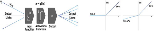
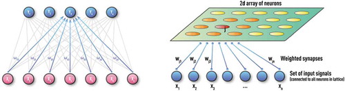
NN consists of a large collection of interconnected processing units, neurons, as shown in Figure 1. Each neuron can receive inputs from one or many other neurons via connections, known as synapses. If the sum of all inputs becomes larger than a certain threshold, a neuron fires (i.e. the neuron sends a signal to other neurons to which it is connected). In general, this process is controlled by nonlinear activation, described by a transfer function, where sigmoid and/or rectified linear functions are often used in practice. NN learns by adjusting the strength of each connection (synapse). Artificial NN ignores a huge fraction of the detailed mechanisms operating in the real brain. One mechanism is thought to be very important for information exchange and processing. A neuron not just fires, but sends a train of electrical spikes [32]. However, this pulse-train generation and other mechanisms of the real neural network are not yet fully adopted into the mainstream models of NN architectures.

Figure 1. Schematic of a typical neuron-like computational unit used in NN architectures. Each neuron can receive inputs from one or many other neurons via connections, known as synapses. If the sum of all inputs becomes larger than a certain threshold, a neuron fires (i.e. the neuron sends a signal to other neurons to which it is connected). In general, this process is controlled by nonlinear activation, described by a transfer function, where sigmoid (left panel) and/or rectified linear (right panel) functions are often used in practice.

Over more than half a century, a large number of different NN configurations with various training procedures and application areas have been proposed. Classification of NN types includes supervised vs unsupervised, feed-forward vs recurrent, as well as many hybrid architectures. Generic examples of the most common practical types of NN are shown in Figures 2–4. A Kohonen NN or Self-Organizing Map (SOM), trained by competitive unsupervised learning algorithms, is successfully used in the clustering of unlabeled data and in the discovery of low-dimensional representations [9,30,33]. A Multi-Layer perceptron (MLP) is a feed-forward NN with at least one hidden layer and supervised training procedure, which is usually based on an error back-propagation (BP) algorithm [9,30,34]. MLP can be effective for modeling complex static and time-series data in regression and classification problems. Unlike MLP, a recurrent NN (RNN) can have feedback loops in different parts of the NN structure, including feedbacks skipping one or more layers. RNN can build robust models of complex sequential data (such as time series) using implicit representation in its internal memory. However, training based on a Back-propagation Trough Time (BPTT) algorithm is often problematic (e.g. it can often encounter vanishing- or exploding-gradient problems) [35,36].

Figure 4. Schematic of the recurrent neural network (RNN) with several feedback loops. Unlike MLP, RNN can have feedback loops in different parts of the NN structure, including feedbacks skipping one or more layers. RNN can build robust models of complex sequential data using implicit representation in its internal memory. However, training based on a Back-propagation Trough Time (BPTT) algorithm could often encounter vanishing- or exploding-gradient problems in practice.

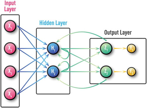
Figure 2. Schematic of unsupervised Kohonen NN or self-organizing map (SOM) with 1D (left panel) and 2D (right panel) architectures. These NNs are trained by competitive unsupervised learning algorithms and used for clustering of unlabeled data and discovery of low-dimensional representations.

Most of the results in NN theory and applications are empirical, even though rigorous mathematical results are often adopted in the training algorithms and other considerations. The original interest in NN was still due to biology and to the assumption that it is possible to adapt several interesting ideas from the nature, even in largely reduced form. However, at least two rigorous mathematical results fully support one’s original intuition about NN as a universal approximation framework. First, Kolmogorov’s theorem formulated in [37] states that every continuous function of several variables (for a closed and bounded input domain) can be represented as the superposition of a small number of functions of one variable. Second, Cybenko’s theorem proves that one-hidden layer feed-forward NN with sigmoid-type activation function is capable of approximating uniformly any continuous multi-variate function to any desired degree of accuracy [38].

However, these two rigorous results do not provide any generic procedure of selecting the appropriate number of hidden-layer nodes and the training of the NN (i.e. finding optimal weights) to achieve a claimed universal approximation of any function. Moreover, the recent shift of NN applications towards deep learning (DL) and deep NN (DNN) leads to even more empirical systems. Namely, there are little to no rigorous theoretical results proving convergence and other properties of the deep-learning formulations [39].

The well-known problem of NN training is the curse of dimensionality [9,30]. In particular, any increase in the number of factors (inputs) in any NN-based or other data-driven model specification requires more training data for the adequate estimation of the model: the number of data samples per model parameter or factor should not dramatically decrease. In the context of NN-based formulation, the dimensionality of the problem (i.e. the number of features or the number of nodes in the input layer) directly leads to an increase of NN weights that should be estimated using available data. In practice, this could easily lead to severe data incompleteness. Also, the error function in the high-dimensional space becomes more complex with increasing number of hard-to-avoid local minima as shown in Figure 5.

The main supervised NN architecture, MLP, is trained using a back-propagation algorithm (i.e. backward propagation of errors) [34]. The main concept underlying this training algorithm is that, for a given observation, one determines the degree of ‘responsibility’ that each network parameter has for each wrong prediction of a target value; the parameters are changed accordingly to reduce NN error. NN training via back-propagation is formalized as a stochastic gradient descent (SGD), as shown schematically in Figure 6 [9]. The iterative NN training is done by presenting known input-output pairs (training samples), calculating the NN error E, and updating the weights w_t as follows:

(1) $w_t=w_{t-1}-\eta \frac{\mathrm{\partial }E}{\mathrm{\partial }w}+\alpha \mathrm{\Delta }{w}_{t-1}$(1)

Figure 6. Schematic of classical gradient descent in 1D (left panel) and stochastic gradient descent (SGD) in 2D (right panel) which is used in NN training with error back-propagation algorithm.

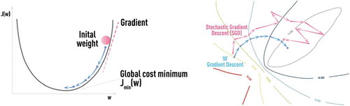
Here, learning rate η and momentum α are user-defined parameters. Updating weights after the introduction of each new sample could often cause excessive noise in the training procedure and could result in much slower convergence. Therefore, epoch (batch) training is frequently used in practice, where error keeps accumulating but weight updating is done only after an ‘epoch’ of N samples. The optimal value of epoch size N is problem dependent (it could easily be several hundred or more).

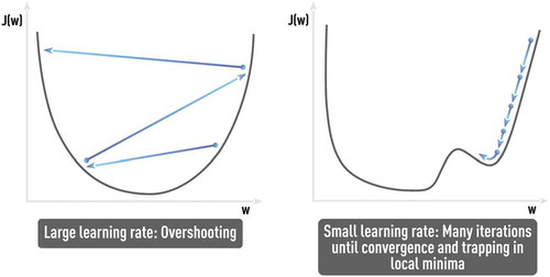
Stochasticity, naturally introduced in SGD by considering errors from only part of training samples at a time, helps escaping saddle points (see Figure 7), which presents a real obstacle for regular gradient descent methods since the gradient vanishes therein. However, finding the optimal SGD parameters that avoid such problems, as ‘trap in local minima’ or ‘very noisy and slow convergence (if any)’, could be challenging and application-dependent without any single universal solution (see schematic in Figure 8).

Figure 7. Schematic of saddle point with vanishing gradients. Stochasticity, naturally introduced in SGD by considering errors from only part of training samples at a time, helps escaping saddle points which presents a real obstacle for regular gradient descent methods suffering from vanishing gradients.

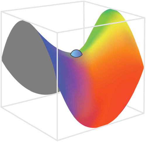
Figure 8. Problems of sub-optimal learning rate (large and small). Finding the optimal SGD parameters that avoid such problems, as ‘trap in local minima’ or ‘very noisy and slow convergence (if any)’, could be challenging and application-dependent without any single universal solution.

3. Regularization, structural risk minimization and support vector machines

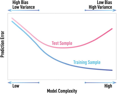
A regularization term always includes one or more parameters that have to be chosen, based on the final objective of the estimated model. In most cases, the objective is the achievement of optimal, or good, out-of-sample performance of the model. The most direct way of estimating out-of-sample error and choosing one or more regularization parameters is to use a validation data set that is not dually used in model training/estimation. Typical bias-variance tradeoff when choosing optimal model complexity is illustrated in Figure 9. The model error on the training set will continue decreasing with increasing model complexity. However, a minimum testing error will be achieved at some optimal value of model complexity.

Figure 9. Schematic of bias-variance tradeoff. Generic behavior of model error computed on test and training samples for different degrees of model complexity. The model error on the training set will continue decreasing with increasing model complexity. However, the minimum testing error is achieved at some optimal value of model complexity.

For more efficient usage of often-incomplete data, one can re-use a training set for out-of-sample error estimation by dividing N training samples into K sets of equal size, training the model on a combination of (K-1) sets, and estimating test error on the remaining sample not being used in training. This procedure, called K-fold cross-validation, is repeated K times; the final test error is an average of test errors for each of K hold-out samples [9,30]. Cross-validation can be applied to any type of model without any limitations. More computationally intensive, cross-validation with N sets (i.e. when just one sample is held out each time) is called leave-one-out cross-validation [9,30].

The cross-validation, or separate validation, set offers a direct way of estimating test error and determining optimal regularization parameters. However, test data used in these estimations is still incomplete and could be biased, which makes test error estimation not very reliable. Also, these estimations could be computationally expensive for some model formulations. Various information criteria (IC) offer an approach for model selection without direct calculation of the test error estimate [30,40]. All these criteria (e.g. the Akaike information criterion (AIC), the Bayesian information criterion (BIC), and their variations) use various penalty terms for model complexity [30,40]. The important limitation of most IC is that they are originally formulated for linear models based on maximum likelihood estimations, and could become less informative or practical where an extension to the more general models is possible. Also, all these measures are asymptotic (i.e. they are applicable only to large samples (N → ∞)) and could often be misleading in real applications with limited data [30,40].

The Vapnik-Chervonenkis (VC) dimension [41,42] offers an alternative model-complexity measure that is fundamentally different from IC metrics on several counts. First, the VC dimension applies to any finite size sample (i.e. it is not an asymptotic measure). Second, the VC dimension applies to any model, not just linear ones. Finally, based on the VC dimension, generic upper bounds for the test (out-of-sample) error can be derived and used in model selection.

Although it is hard to compute the VC dimension for an arbitrary set of functions, simulations can be used for estimation. VC dimensions and corresponding test-error bounds are the basis of the Structural Risk Minimization (SRM) principle which is at the core of Support Vector Machine (SVM) and other formulations of large-margin classifiers [41–44].

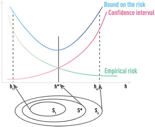
Test-error bounds, based on the VC dimension, are keys to the SRM approach. Empirical Risk Minimization (ERM) used in most ML algorithms is based on training (i.e. in-sample) error. SRM directly incorporates an upper-bound estimate of the out-of-sample error into the estimation/training process. As illustrated in Figure 10, SRM fits a nested sequence of models of increasing VC dimensions h₁ < h₂ < … < h_n and then chooses the model with the smallest value of the upper-bound estimate. Algorithms (like SVM) that are based on the SRM principle incorporate regularization that is aimed at better out-of-sample performance, into the training procedure itself. However, even SRM-based algorithms could benefit from additional regularizations. One example of such regularization is the soft-margin parameter used in SVM which is critical in practical classification problems having overlapping classes [41,42,44].

Figure 10. Schematic of optimal model selection using the principle of structural risk minimization (SRM). SRM fits a nested sequence of models of increasing VC dimensions h1 < h2 < … < hn and then chooses the model with the smallest value of the upper-bound estimate. Algorithms (like SVM) that are based on the SRM principle incorporate regularization that is aimed at better out-of-sample performance, into the training procedure itself.

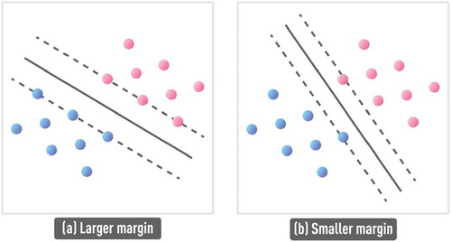
While algorithmic and theoretical details behind SVM formulation are beyond the scope of this paper, Figure 11 provides a simple illustration of the SRM result in the SVM context. First, the SVM algorithm involves a kernel transform that casts the nonlinear classification problem to a higher (or even infinite) dimensional space where this problem becomes linearly separable. Next, support vectors define boundaries of the classes and the decision hyperplane (or line in 2D) is specified to be equidistant from the two support vectors. As shown in Figure 11, the SVM algorithm, based on SRM principle, can find the optimal support vectors and the corresponding decision boundary to ensure large separation (i.e. large margin) between classes, ensuring good out-of-sample performance.

Figure 11. Schematic of larger margin classifier (a), compared to smaller margin classifier (b). Support vectors (dashed lines) define boundaries of the classes and the decision hyperplane (solid line) is specified to be equidistant from the two support vectors. SVM algorithm, based on the SRM principle, can find the optimal support vectors and the corresponding decision boundary to ensure large separation (i.e. large margin) between classes, ensuring good out-of-sample performance.

Even when the VC dimension is hard to compute, the main SRM principle (i.e. ‘optimizing the worst case’) can be applied across a much wider range and in different statistical and ML algorithms. This can be done via the appropriate choice of challenging optimization objectives.

However, in many cases with extreme data limitations, it is impossible to find an adequate solution without the usage of domain knowledge and other prior information. This is conceptually illustrated in Figure 12, where available noisy data (red circles) for the unknown quadratic function y = ax² (blue line) cover a very limited range. In this case, it is impossible to choose the correct complexity of the fitting model (for extrapolation) without incorporating any additional information.

Figure 12. Schematic of quadratic dependence estimation from a very limited data set with and without domain knowledge about the estimated function. Available noisy data (red circles) for the unknown quadratic function y = ax² (blue line) cover a very limited range. It is impossible to choose the correct complexity of the fitting model (for extrapolation) without incorporating any additional information. Most statistical algorithms would choose linear regression (orange line) with bad out-of-sample performance. However, if domain knowledge hints to quadratic nature of the functional form, estimating the parameter a in y = ax² from a few available data points leads to low-complexity model (grey line) with very good out-of-sample performance.

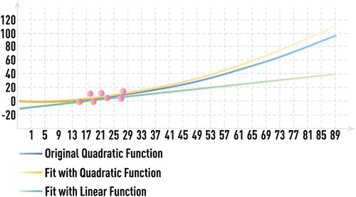
Most statistical algorithms would choose just a linear regression in this case (orange line), which would give large prediction errors outside of the range of training data. However, if there is domain expert knowledge indicating that the considered effect can be expressed by a quadratic function, estimating the parameter a in y = ax² from a few available data points and obtaining a calibrated low-complexity model (grey line) having very high out-of-sample accuracy and stability would be straightforward.

Optimal choice of the objectives (e.g. training-algorithm ‘loss’ function) to find a solution with good generalization capabilities can also be considered as a type of regularization. Often, direct usage of the final problem-specific objective as an algorithm objective (the training-algorithm loss function) may not be an optimal choice. As already mentioned, the broad interpretation of the SRM principle indicates that focusing on optimizing avoidance of worst possible cases (e.g. minimizing tails of error distributions), may provide a much more stable out-of-sample solution, according to the original objective compared to directly employing the training-algorithm loss function as the objective. This was earlier illustrated in the context of discovering optimal boosting-based trading strategies [45] where, instead of direct usage of obvious objectives such as strategy return at the horizon of interest and/or the Sharpe ratio, much more stable out-of-sample solutions are found by optimizing (i.e. minimizing) the lower tail of the distribution of returns on much smaller horizons (i.e. worst results).

4. Ensemble learning, boosting, and generalized degrees of freedom

The practical value of the model combination is exploited by practitioners and researchers in many different fields. The basic idea of ensemble learning algorithms is to combine relatively simple base hypotheses (models) for the final prediction. The important question is why and when an ensemble is better than a single model. In machine learning literature, three broad reasons for the possibility of good ensembles’ construction are often mentioned. First, there is a pure statistical reason. The amount of training data is usually too small (data incompleteness) and learning algorithms can find many different models (from model space) with comparable accuracy on the training set. However, these models capture only certain regimes of the whole dynamics or mapping that becomes evident in out-of-sample performance. There is also a computational reason related to the learning algorithm specifics such as multiple local minima on the error surface (e.g. NNs and other adaptive techniques). Finally, there is a representational reason when the true model cannot be effectively represented by a single model from a given set even for the adequate amount of training data. Ensemble methods have a promise of reducing these key shortcomings of standard learning algorithms and statistical models.

The advantage of the ensemble learning approach is not only the possibility of the accuracy and stability improvement of pure data-driven models, but also its ability to combine best features of a variety of models: analytical, simulation, and data-driven. This latter feature can significantly improve the explanatory power of the combined model if building blocks are sufficiently simple and based on well-understood models. However, ensemble learning algorithms can be susceptible to the same problems and limitations as standard machine learning and statistical techniques. Therefore, the optimal choice of both the base model pool and the ensemble-learning algorithms, ideally having good generalization qualities and tolerance to data incompleteness and dimensionality, is very important.

An ensemble-learning algorithm that combines many desirable features is boosting [18,43]. Boosting and its specific implementations such as AdaBoost [46] have been actively studied and successfully applied to many challenging problems. One of the main features that set boosting aside from other ensemble-learning frameworks is that it is a large-margin classifier similar to SVM. This ensures superior generalization ability and better tolerance to incomplete data compared to other ensemble-learning techniques. Statisticians consider boosting as a new class of learning algorithms that Friedman named ‘gradient machines’ [7], since boosting performs a stage-wise, greedy, gradient descent. This relates boosting to particular additive models and to matching pursuit, known within the statistics literature [19,30].

The main practical focus is on the ensemble-learning algorithms suited for challenging problems dealing with a large amount of noise, limited number of training data, and high-dimensional patterns [43]. Several modern ensemble learning techniques relevant for these types of applications are based on training-data manipulation as a source of base models with significant error diversity. These include such algorithms as bagging (‘“bootstrap aggregation”’), cross-validating committees, and boosting [30,43].

Bagging is a typical representative of ‘“random sample”’ techniques in ensemble construction. In bagging, instances are randomly sampled, with replacement, from the original training dataset to create a bootstrap set with the same size [30]. By repeating this procedure, multiple training-data sets are obtained. The same learning algorithm is applied to each data set and multiple models are generated. Finally, these models are linearly combined (averaged) with equal weights. Such combination reduces the variance part of the model error as well as the instability caused by the training set incompleteness. Bagging exploits the instability inherent in learning algorithms. For example, it can be successfully applied to the NN-based models. However, bagging is not efficient for the algorithms that are inherently stable, that is, whose output is not sensitive to small changes in the input (e.g. parsimonious parametric models). Bagging is also not suitable for a consistent bias reduction.

Intuitively, combining multiple models helps when these models are significantly different from one another and each one treats a reasonable portion of the data correctly. Ideally, the models should complement one another, each being an expert in a part of the domain where the performance of other models is not satisfactory. The boosting method for combining multiple models exploits this insight by explicitly seeking and/or building models that complement one another [18,43,47]. Unlike bagging, boosting is iterative. Whereas in bagging, individual models are built separately, in boosting, each new model is influenced by the performance of those built previously. Boosting encourages new models to become experts for instances handled incorrectly by earlier ones. The final difference is that, in boosting, adjusted weights are assigned to models by their performance (i.e. the weights are not equal as in bagging). Unlike bagging and similar ‘“random sample”’ techniques, boosting can reduce both bias and variance parts of the model error. Using probably-approximately-correct (PAC) theory, it was shown that, if the base learner is just slightly better than random guessing, AdaBoost is able to construct an ensemble with arbitrarily high accuracy [47]. Thus, boosting can be effective for constructing a powerful ensemble from very simplistic ‘rules of thumb’ known in the considered field (i.e. domain-expert knowledge).

Boosting-based models demonstrate very good out-of-sample accuracy and stability, even in cases having limited training data due to any intrinsic property of margin maximization during training. A typical boosting algorithm such as AdaBoost [46] for the two-class classification problem (+1 or −1) consists of the following steps:

for n: = 1,…, N

(2.1) $w_n^1=1/N$(2.1)

end

for t: = 1,…, T

(2.2) ${\epsilon }_t=\sum _{n=1}^N\left(w_n^{t}I(-y_n{h}_t(x_n))\right)$(2.2)

(2.3) ${\alpha }_t=\frac{1}{2}ln\left(\frac{1+{\epsilon }_t}{{\epsilon }_t}\right)-\frac{1}{2}ln\left(\frac{1+\rho }{1-\rho }\right)$(2.3)

(2.4) $w_n^{t+1}=w_n^{t}exp\left(-{\alpha }_t{y}_n{h}_t(x_n)\right)/Z_t$(2.4)

and

(2.5) $H(x)=\sum _{t=1}^T{\alpha }_t{h}_t(x)/\sum _{t=1}^T{\alpha }_t.$(2.5)

Here N is the number of training data points, x_n is a model input value of the n-th data point and y_n is class label, T is the number of iterations, I(z) = 0 (z <0), I(z) =1 (z >0), w_n^t is the weight of the n-th data point at t-th iteration, Z_t is normalization constant, h_t(x_n) is the best model at the t-th iteration, ρ is a regularization constant, and H(x) is the final combined model (meta-model).

Boosting starts with equal and normalized weights for all training samples (step 2.1). Base classifiers h_t(x) are trained using weighted error function ε_t (step 2.2). The best h_t(x) is chosen at the current iteration. The adjusted data weights for the next iteration are computed in steps (2.2)-(2.4). At each iteration, data points misclassified by the current best model (i.e. y_n h_t(x_n) < 0) are penalized by the weight increase for the next iteration. AdaBoost constructs progressively more difficult learning problems that are focused on hard-to-classify patterns defined by the weighted error function (step 2.2). Steps (2.2)-(2.4) are repeated at each iteration until stop criteria occur. The final meta-model (Equation (2.5)) classifies the unknown sample as class +1, when H(x) > 0, and as −1, otherwise.

From the above description, it is clear that a typical boosting algorithm is based on the utilization of low-complexity base models estimated one at a time and deterministic iterative approach where initial discovery of the best-on-average model is followed by additions of models focused on more challenging data patterns/regimes that were poorly modeled in previous iterations [10,46]. Therefore, similar to DNN-based DL, discussed in the next section, boosting takes advantage of hierarchical knowledge representation and independent training of the model components.

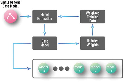
In pure data-driven approaches, a typical choice of the base model represents a decision stump (i.e. one-level decision tree) as shown in Figure 13 where the boosting procedure is diagrammed. In this case, just one generic, application-independent, base model is used. The final model is a multi-level tree constructed over many boosting iterations. However, the out-of-sample performance of such large tree discovered by boosting is much better than that of the same tree obtained by simultaneous global optimization of the parameters of the multi-level tree [30].

Figure 13. Schematics of a generic boosting algorithm with decision stump (i.e. one-level decision tree) as a base model. Such generic, application-independent, base model is a typical choice in pure data-driven approaches.

Generic boosting and its various extensions, such as XGBoost [8], often demonstrate superiority over other algorithms in many applications and competitions. Its performance often approaches that of DNN. Since the discovery of a boosting-based solution may often be operationally simpler, there are legitimate arguments in favor of choosing boosting rather than DNN in certain applications. However, as discussed in subsequent sections, many hybrid approaches try to combine the best features of boosting and DNN rather than choose just one approach and discard the other.

Generic boosting algorithms, such as shown in Figure 13, are flexible but still require a significant amount of training data for the discovery of accurate and stable models. Domain-expert models and other existing knowledge obtained by a deeper understanding of the considered domain could play a key role in applications with severe incompleteness of training data due to natural dimensionality reduction and usage of domain-specific constraints. However, such simplified models are often biased and incapable of covering all possible regimes. On the other hand, comprehensive incorporation of this domain knowledge, such as analytical models, rules or constraints, into a majority of machine learning algorithms, including the generic boosting algorithm shown in Figure 13, is problematic, except when providing straightforward guidance in factor selection. However, boosting can be applied to the pool of the well-understood and low-complexity domain-expert models to produce an interpretable ensemble of complementary base models with significantly higher accuracy and stability as suggested in [10–14]. A schematic of such an algorithm is shown in Figure 14.

Figure 14. Schematics of boosting algorithm with multiple well-understood and low-complexity domain-expert models as base models. Such a procedure can test and utilize the complementary value of any number of available domain-expert models without overfitting. Proper parameterization could also allow discovery of many complementary models, even from a single domain-expert model.

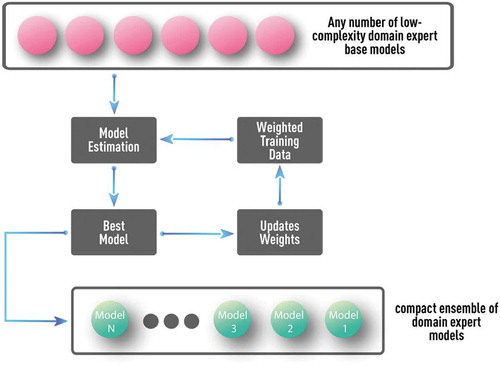
Unlike generic boosting algorithms (such as in Figure 13), the pool of base models could include any number of parameterized domain-expert and/or other low-complexity models (see Figure 14) [10–14]. At each boosting iteration, all models from this pool are optimized, one at a time, according to the weighted error function, and the best model is added to the ensemble. Such a procedure can test and utilize the complementary value of any number of available domain-expert models without overfitting. Also, proper parameterization could allow discovery of many complementary models, even from a single domain-expert model. Unlike boosting with generic and simple tree-based model, domain-expert base models could already capture a significant number of regimes and impose important application-specific constraints. This facilitates the discovery of compact model ensembles that combine high accuracy with interpretability since well-understood base models are used [10–14].

It may seem counter-intuitive that the final boosting ensemble with potentially dozens or hundreds of base models demonstrates superior out-of-sample performance. One can argue that the complexity of such an ensemble is much higher than that of any single base model and one can expect severe overfitting. However, complexity of boosting ensemble does not scale up with the number of base models as would be the case in a single linear model with increasing number of inputs (parameters). Due to component-wise discovery of such ensemble (i.e. one model at a time is estimated), the generalized degrees of freedom (GDF) measure [48] is often just slightly above that of a single base model or could be even less than GDF of the base model. This effect of low complexity of the boosting-based ensemble is often referred to as ensemble paradox [48]. Similarly, for a nonlinear model, its GDF is not, in general, equal to the number of adjustable parameters (such as weights in NN). As discussed in the next section, the main difference and advantage of DL, compared to standard NN, is component-wise (layer-by-layer) learning. Therefore, DNN trained with DL approach may be very large; however, still it can show superior out-of-sample performance. This means that the learning procedure itself warrants the low GDF of the final NN-based model.

However, even though boosting seems to be more natural for incorporation and enhancement of the domain-expert knowledge, its flexibility is still inferior to DNN-based DL. After all, boosting determines a weighted linear combination of models. While such combination is capable of representing very complicated (non-linear) decision boundaries in classification problems, it may still miss important mixed terms that could be easily captured by flexible DNN representation. Also, in many modern applications, performance of tree-based ensemble learning algorithms [8,25] can be drastically increased by using feature engineering procedure before the actual application of ensemble learning. The number of generated features could be significantly higher than the number of original features. Similar to kernel-based techniques like SVM, this allows reformulating the original classification problem in higher dimensional space with simpler and less nonlinear decision boundaries which helps classification algorithm in constructing a more accurate model. However, unlike almost analytical kernel-based approaches, general feature engineering is often outside of ensemble learning algorithm itself and could be very empirical without any warranty of out-of-sample stability. Therefore, typically, feature engineering process should be repeated when significant amount of new data become available. On the other hand, unsupervised part of DNN (auto-encoders), is an integral part of DL framework and generated hierarchical representations (feature extraction) could be more self-consistent and stable. Therefore, DNN-based DL and its combination with boosting could offer many advantages in modeling complex data and systems as discussed next.

5. Deep learning

Many properties of NN have been discovered well before the current resurgence of interest in these algorithms in the form of DL and DNN. For example, formal mathematical results of NN universality and their capabilities have been proven by Kolmogorov and Cybenko [37,38]. Cybenko’s theorem states that feed-forward NN, with just one-hidden layer and one sigmoid activation function, is capable of approximating uniformly any continuous multivariate function to any desired degree of accuracy [38]. However, these results do not provide any direct recipes for determining the optimal NN for any given problem and training data.

Based on Cybenko’s theorem, the optimal NN having good approximation should exist for any problem that meets reasonable continuity requirements. However, the multi-factor nature of the majority of practical problems leads to the set of challenges that are collectively called the curse of dimensionality [9,30]. In the context of NN, the large number of weights and complex error surface with many local minima is responsible for this challenge [9]. A direct global optimization of NN weights for avoiding local minima cannot solve the problem because of high-dimensionality of the problem, which is prohibitive to any stochastic or heuristic optimization algorithms, including Genetic Algorithms (GA). Only after iterative back-propagation (BP) algorithm cycles for training NN with any number of hidden layers, as proposed in [34], many practical NN-based applications emerged.

However, while BP was routinely and successfully used for NN training in many practical situations, discovery of optimal NN in each particular application still faced many serious challenges without a single universal solution. Many problems such as vanishing or exploding gradients are limitations of BP algorithm and can be encountered in many NN architectures including well-known multi-layered perceptron (MLP) [34–36]. Some NN types may provide a very powerful modeling framework but are especially hard to train in practice. For example, while recurrent NN (RNN) could potentially find the best solutions in problems dealing with time series and general sequence forecasting, the training algorithm, back-propagation through time (BPTT), could be notoriously unstable in practice [35,36].

Active research efforts to resolve or alleviate these limitations of NN-based frameworks, and machine learning algorithms in general, resulted in the development of modern DNN-based DL approaches [5,6]. Widespread adoption of DL frameworks began after 2012 when AlexNet (convolutional DNN) significantly outperformed other machine-learning approaches in the ImageNet Large Scale Visual Recognition Challenge [49]. This result facilitated explosive growth of DNN-based applications in computer vision, bioinformatics, healthcare, fundamental sciences, business and other areas [5,6,24].

DNN are often regarded simply as multi-layered NN which were made available for real-world applications because of the possibility to train them with modern computing resources, such as massively parallel GPU-based systems (www.nvidia.com). However, the main advantage of DL, capable of alleviating many existed issues, comes from the structured approach to DNN training and hierarchical representation which can be outlined as follows [5,6].

DNN-based DL is not just NN with large number of hidden layers. It is an important paradigm that realizes the importance of hierarchical representation of data that have an increasing degree of abstraction [5,6,22]. This paradigm is not new for fundamental sciences, where theoretical and simulation frameworks are often focused on different spatiotemporal scales and account for interaction (energy flow) across these scales. For example, the success of realistic simulations of multi-scale spatiotemporal dynamics in plasma and space physics critically depend on proper formulation and coupling of physical models that describe processes on micro- and macro scales, since it is infeasible to model a wide range of scales from first principles because of computational limitations and lack of detailed initial/boundary conditions [e.g. 50].

In the traditional machine learning (ML), the process of feature selection could often include such hierarchical representations without explicit formalization. As already discussed, boosting-like ensemble learning is an example of an intrinsically hierarchical algorithm. It starts from a global-scale classification/regression model at the first iteration and focuses on more detailed modeling of sub-populations and sub-regimes in subsequent iterations [10].

Although NN-based implementation of DL paradigm is not the only choice, DNN provides a universal framework for modeling complex and high-dimensional data. An especially attractive feature of the DNN approach is the capability of covering all stages of data-driven modeling (features selection, data transformation, and classification/regression) within a single framework (i.e. ideally, the practitioner can start with raw data in the domain of interest and obtain a ready-to-use solution) [5,6].

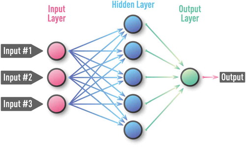
The key difference between standard multi-layered NN and DNN-based DL is illustrated in Figure 15. As an example of a standard NN framework, schematic MLP diagram is shown in Figure 3. In this case, input features/factors presented to NN in the first layer are assumed to be already selected outside NN by other means, ranging from simple correlation analysis, to different flavors of principal component analysis (PCA), and to other statistical and machine learning tools (e.g. [30]). Once inputs are chosen, one can start supervised training of MLP using BP algorithm. In this training procedure, all adjusted weights from all layers are updated at each BP iteration or epoch [9,34].

Figure 15. Schematics of DNN with stacked auto-encoders followed by supervised NN. First, the auto-encoder layers are trained in unsupervised fashion using labeled and unlabeled data. Then, the MLP classifier is trained on labeled data using usual supervised learning, while weights from the first set of layers are kept constant. For further reduction of requirement on training data size, single multi-layer auto-encoder is replaced by a stack of shallow auto-encoders (e.g. each with only one hidden layer) that are trained one at a time.

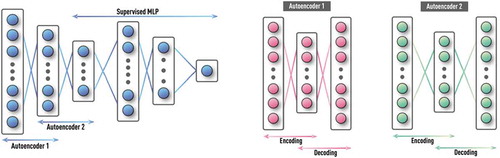
Figure 3. Schematic of a supervised feed-forward neural network also known as multi-layer perceptron (MLP). MLP is a feed-forward NN with at least one hidden layer and supervised training procedure, which is usually based on an error back-propagation (BP) algorithm. MLP can be effective for capturing complex patterns in both regression and classification problems.

The obvious limitation of this standard NN framework is the absence of universal approaches to feature selection and dimensionality reduction that would be a self-consistent part of the framework itself and applicable in any domain of interest. Large dimensionality of inputs directly translates to a large number of adjusted weights. Since the adjusted weights of all layers are updated simultaneously, the already-mentioned problems of having a large number of hard-to-avoid local minima on the multi-dimensional error surface, vanishing and/or exploding gradients, and related problems are easily encountered in many practical applications.

A DNN-based DL alternative to standard MLP is schematically shown in Figure 15. The obvious difference from Figure 3 is an additional set of layers before the actual MLP layers for classification/regression. These additional layers effectively perform generic feature selection and dimensionality reduction via unsupervised pre-training, filtering and input transformations [5,21,22,51]. In some cases, this pre-processing may include a domain-specific set of filters and transformations such as in CNN-based DL for image recognition [49]. However, the most generic application-independent approach is based on auto-encoders, as illustrated in Figure 15.

Auto-encoder in its basic form is equivalent to MLP, with output layer equal to the input layer [21,22,51]. The training is based on the standard BP used in supervised MLP training. The only difference is that input features are presented at both input and output layers during training, i.e. NN builds representation of its input in hidden layer(s) (as part of the encoding process) and then tries to recover the original input from this representation (as part of the decoding process) as schematically shown in Figure 15. Since only inputs are used in training, it is, effectively, unsupervised learning. Typically, the number of nodes in the hidden layer(s) is significantly less than the number of inputs. In this case, the auto-encoder discovers a compact representation of the original input information (i.e. performs generic dimensionality reduction). However, if the objective is to discover sparse representations uncovering complex non-linear dependencies (patterns), then the size of a hidden layer is made larger than the number of inputs. In the final NN, only the encoding layers of auto-encoders are used, as shown in Figure 15.

Unsupervised pre-training of DNN, using auto-encoders or other approaches, is even more important in applications with a large amount of unlabeled data but more limited availability of labeled data, which is often the case. Indeed, standard supervised learning would use only labeled data, while information contained in the unlabeled data is ignored. Unsupervised pre-training is capable to discover rich set of patterns and representations from unlabeled data. After that, DNN could be further fine-tuned via supervised training using available labeled data.

Thus, while the NN structure in standard MLP and DL approaches may look the same, the key difference of true DL is that NN is trained layer-by-layer, which leads to much more robust results and alleviates potential overfitting. First, the set of layers (e.g. auto-encoders) are trained in unsupervised fashion with the ability to use most of the data (labeled and unlabeled). Then, the MLP classifier is trained using usual supervised learning, while weights from the first set of layers are kept constant. Finally, one could choose to fine-tune all NN layers with supervised training on labeled data.

Important concept of layer-by-layer learning in DNN goes well beyond just two major groups of layers, that is, with unsupervised (e.g. auto-encoders) and supervised (e.g. standard MLP) learning. This allows further alleviation of often-encountered problems due to data incompleteness. For example, while one can train single auto-encoder with multiple hidden layers, this approach would have serious problems in practice, if the data is limited. Therefore, an often used alternative is a stack of shallow auto-encoders (e.g. each with only one hidden layer) that are trained one at a time [22]. The example in Figure 15 shows a stack with two such auto-encoders.

Another robust technique of layer-by-layer training is transfer learning, with many practical applications in image recognition and other fields [52–54]. For example, millions of images in hundreds of categories are available for DNN training. However, one may have just a few hundred images in the domain of interest, such as medical imaging for a particular abnormality [52,53]. In this case, NN is first pre-trained on available categories not directly related to the problem of interest. Then one could keep weights constant in a majority of initial layers and train just a few last layers (in MLP) on available medical images. This is transfer learning, since we transfer majority of patterns learned in the domain with large data set (i.e. abstract image descriptors) to a different domain with small data set. Only a small fraction of final layers gets updated. Depending on the data availability for the actual problem, one may increase or decrease the number of updated layers (weights). In the extreme case of very limited data set, one can even replace MLP layers with a simpler model (i.e. logit regression or a support vector machine).

However, severe data limitations in the context of problem dimensionality and/or absence of relevant problem for transfer learning can still drastically reduce key advantages of DNN-based DL. For example, pure data-driven auto-encoders dealing with high-dimensional input data require a large amount of data for effective operation.

Even when the problem with training-data completeness is not critical, the other serious challenge is finding optimal hyper-parameters and NN configurations. For every data set, there is a corresponding NN that performs ideally with that data. However, there is no universal procedure for the efficient and fast discovery of optimal hyper-parameters and DNN configurations, due to too many possible combinations: learning and momentum rates (see Equation (1)), regularization types and parameters (e.g. weight decay constant), epoch/batch size, number of layers in unsupervised and supervised parts, number of nodes in each layer, and others. Hyper-parameter selection may be significantly accelerated if the existing domain knowledge can be efficiently used as guidance. However, in general, it is not warranted, and practitioners have to use a grid search, which cannot be applied to high-dimensional hyper-parameter space due to a combinatorial explosion of available combinations, requiring a random search where no information from previously considered solutions are used, and a true optimization with some heuristic algorithms, including GA-based and other multi-objective optimization approaches. In any case, if domain-expert guidance is absent, determining optimal hyper-parameters and DNN configurations become extremely time-consuming and computationally intensive, even when each DNN configuration during this optimization procedure is trained using a powerful GPU system.

6. Single-example learning and ensemble decomposition learning for representation and prediction of complex and rare patterns

Rare and complex states, abnormalities or regimes cannot be adequately quantified even by the most advanced machine-learning approaches that are capable of minimizing requirements on calibration/training data. This is because of the very nature of these states – they may have just a single or a few training examples. However, the human brain is capable of classifying objects from the novel class even after a single example from that class is presented. Such capabilities of the human brain are explained by the similarity representation of the novel class to many well-learned classes. A similar approach is known in computer science as a representation by similarity [13,55]. Novel class is represented as a vector of probabilities of N well-known classes to which a novel example belongs. Schematic illustration of such a representation is shown in Figure 16.

Figure 16. Schematic of representation by similarity. Novel class (llama) is represented as a vector of probabilities of three well-known classes (giraffe, sheep, and dog) to which a novel example belongs.

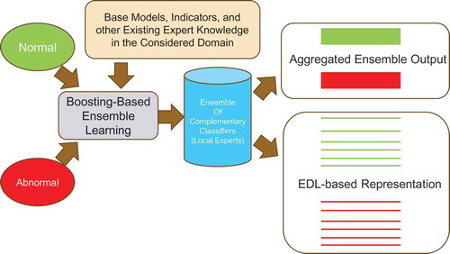
Representation by similarity allows Single-Example Learning (SEL) of novel or rare classes/states/regimes. However, it still requires a significant number of known classes with many examples. Nevertheless, boosting applied even to a two-class problem (e.g. ‘normal’-'abnormal') produces an ensemble of many complementary classifiers that represent many implicit sub-classes or regimes within these two classes. A vector of these complementary models could offer a universal representation, by similarity for many rare and complex cases, with limited number of known examples. We called such decomposition of the boosted ensemble, Ensemble Decomposition Learning (EDL) which can be interpreted as follows [13].

Good performance of the final boosting-based ensemble model is achieved by building and combining complementary models that are experts in different regions of feature space or in regimes of the considered complex system. Therefore, many unspecified regimes are learned implicitly. However, only the aggregated output of the ensemble is used in standard approaches, while the rich internal structure of the meta-model remains completely ignored. We proposed the methods for extraction of that implicit knowledge and called this framework EDL [13].

If the final aggregated classifier H(x) is given by Equation (2.5), one can introduce the ensemble decomposition feature vector as follows:

(3) $D(x)=[{\alpha }_1{h}_1(x),{\alpha }_2{h}_2(x),...,{\alpha }_T{h}_T(x)]$(3)

Here, we assume that α_i are already normalized as explicitly specified in Equation (2.5).

Each sample, after the ensemble classification procedure, can be represented by this EDL vector D(x). This vector can provide detailed and informative state representation of the considered system which is not accessible in the aggregated form H(x). The functions h_i(x) are local experts in different implicit regimes or domains of a whole feature space, which ensures good global performance of the final ensemble. Therefore, it is reasonable to assume that, for similar samples from the same regime, the meta-classifier would give similar decomposition vectors.

Two samples x₁ and x₂ are considered to be similar if their ensemble decomposition vectors D(x₁) and D(x₂) are close to each other in some metric, for example, l₂ norm, i.e.

(4) $∥D(x_1)-D(x_2)∥<\delta$(4)

This approach can be especially useful in applications where the significant limitation of data with clear class labels makes it impossible to provide an adequate number of reference classes required for standard SEL techniques [13,55].

The aggregated output of the boosted ensemble provides good separation of the considered classes (e.g. normal – abnormal). Sub-classes or sub-states within these two classes are not well separated. It cannot be applied to differentiate between other classes which were not used in training. The EDL vector provides universal and fine-grain representation not only for the two learned classes but also for sub-classes/sub-states within these two classes, as diagrammed in Figure 17.

Figure 17. Schematic of classical boosting-based ensemble learning and ensemble decomposition learning (EDL) based on the boosting ensemble. The EDL vector provides universal and fine-grain representation not only for the two learned classes but also for sub-classes/sub-states within these two classes.

It should be noted that DNN-based DL frameworks do not offer any direct and generic means to handle SEL problems in a consistent and universal manner. However, recently we have shown that standard results of the aggregated ensemble can be enhanced by a combination of the best features of boosting and DNN [23]. Similarly, our preliminary results indicate that DNN is capable of enhancement of EDL effectiveness which will be reported elsewhere.

III. Synergy of physics-based models and machine learning in biomedical applications

Practical quantitative modeling of most adaptive complex systems with many interacting components presents serious challenges [11–14]. Insufficient accuracy of both the simplified analytical, and other low-complexity models, and the empirical expert-defined rules is a typical limitation of existing domain-expert approaches. Also, even when the problem can be fully described from the first principles and the computation power is abundant, very wide range of scales in realistic systems (many orders of magnitude) could still make direct physical simulation impossible, even for the most powerful multicore CPU/GPU architectures. However, even more important is the fundamental restriction caused by the lack of detailed initial/boundary conditions. Therefore, even when a complex system of interest can be rigorously described by fundamental physical equations, many practical constraints may force to reformulate (‘regularize’) the original problem. Here we do not refer to physics-based frameworks that are routinely used for direct interpretation of data in such diagnostic tools as X-Rays or MRI and where the key role of physics-based frameworks is obvious.

For example, the important problem of space-weather forecasting (i.e. prediction of storms and sub-storms in Earth’s magnetosphere) is very challenging due to the interplay of physical processes of a vast range of time and spatial scales [50]. Besides the obvious drastic limitation of computing power, the fine-grain initial and boundary conditions are not known; it is impossible to have a satellite in every spatial location simultaneously. Therefore, different kinds of model reformulations allow useful practical results to be obtained. Often, small-scale kinetic effects are introduced as anomalous coefficients into large-scale fluid simulations without running small-scale simulations [50]. One can also approximate the whole magnetosphere-ionosphere system as a giant, but a simple, electric circuit with just a few main elements having characteristics inferred from deeper physical models (analog models) [56]. Finally, we can use machine-learning formulations including NN and SVM, where inputs, time-delays, and other characteristics are guided by physics-based models and intuition [57].

Similar challenges are also relevant for physics-based modeling of biomedical systems. For example, modern computers make possible 3D physical simulations of human physiology including the cardiovascular system. While these models may already be useful in certain diseases and drug effects simulations, the inability of precision specification of all required details (system parameters, boundary conditions, etc.) limits the applicability of these simulations to a large class of practical problems. On the other hand, more coarse-grain dynamical models, such as cardiovascular models, can be formulated as a system of ordinary differential equations approximating cardiovascular dynamics by a small number of components and their interactions without a more detailed description (see discussion in section 2.4) [58]. For example, these physics-based approximations allow the practical generation of a very realistic, synthetic, ECG time series for normal and pathological conditions that can be used in various ways as discussed later.

As follows from our short review of modern machine-learning approaches, the main limitations of pure data-driven models come from data incompleteness that prohibits the capturing of all complex patterns of the considered dynamical systems and that still warrants stable out-of-sample performance. Typical problems of complex system modeling, such as the ‘curse’ of dimensionality and non-stationarity, lead to serious challenges in biomedical applications. For example, direct machine-learning models in bioinformatics have very high-dimensional inputs causing training data incompleteness, even with an apparent abundance of the microbiological data [44]. Indeed, training data should include a sufficient part of all possible input combinations, which scales as ~M₁M₂…M_N, where N is total number of inputs (basic features) and M_i is typical number of different ranges/regimes for i-th feature. Similar problems are also relevant for models based on multi-channel and multi-scale physiological data. Non-stationarity is even a more important challenge in modeling physiological dynamics. It is usually impractical to find and calibrate a single global multi-dimensional model that reasonably covers all different dynamical regimes. Also, model interpretability, which is critically important especially in biomedical applications, is often lacking in pure data-driven models.

All modern approaches such as SVM, boosting-based ensemble learning, and DNN-based DL, try to alleviate the problem of data incompleteness and improve out-of-sample performance even in the cases of very limited test data. Even though these advanced frameworks look different, the generic underlying ideas are often very similar. For example, both SVM and boosting are large-margin classifiers even though SVM achieves this by applying a kernel transform for problem linearization, followed by robust classification according to the SRM principle, while boosting maximizes the margin in functional space via a combination of simple complementary models [10,18,30,43,46]. Similarly, component-wise learning and hierarchical representation are key features of achieving superior out-of-sample performance by combined boosting and DNN-based DL [23].

Modern machine-learning approaches are capable of significant alleviation of the key limitation of data-driven models. For example, the kernel transform in SVM decouples the dimensionality of the classification space from the dimensionality of the original input, which made SVM the algorithm of choice in bioinformatics problems having very high dimensionality [44]. Similarly, financial problems (e.g. volatility forecasting) having multi-scale dependencies could also benefit from this SVM feature [59,60]. Now, these problems are also tackled by DNN-based DL frameworks.

Widespread adoption of DNN-based DL frameworks began after 2012 when AlexNet (convolutional DNN) significantly outperformed other machine-learning approaches in the ImageNet Large Scale Visual Recognition Challenge [49]. This success was an example of layer-by-layer training (a distinct feature of DL not present in classical NNs), where unsupervised pre-training module was able to discover many important features from a large multi-million database of labeled and unlabeled images that ensured accurate classification by the supervised part of DNN. Although this success can be legitimately attributed to the existence of a large image database, the obtained results can be further re-used in other image recognition problems using transfer learning concept. For example, if for a particular diagnostic problem, collection of medical images is limited, one can re-use a large part of DNN trained for general image recognition problem and re-train only several last layers of DNN [52,53].

However, severe data limitations in the context of problem dimensionality and/or absence of relevant problem for transfer learning can still drastically reduce key advantages of DNN-based DL. For example, even for an unsupervised pre-training phase, auto-encoders dealing with high-dimensional input data require a large amount of data for effective operation. Also, the variability in physiological dynamics and other biomedical applications could be much higher than in an image-recognition problem. Similar challenges are also relevant for other data-driven frameworks including rare pattern recognition in the context of SEL or EDL [13,55]. For example, for SEL, there is a requirement of large data sets for base classes. In the EDL approach, there is a requirement of large enough data sets for the small number of classes (e.g. normal and abnormal) and a rich set of flexible base models should be available [55]. Therefore, existing domain-expert models/rules obtained by deeper understanding of the considered domain could play a key role in applications with severe incompleteness of training data due to natural dimensionality reduction and usage of domain-specific constraints. In some sense, the usage of domain-expert knowledge could be considered as the ultimate transfer of learning.

Thus, given limitations of both domain-expert models and pure data-driven approaches, it is natural to find synergistic combinations of these approaches where their best features can optimally complement each other. This can be achieved in several different ways. The most open framework for direct incorporation and testing of any complementary value of existing domain-exert knowledge is the usage of existing and properly parametrized analytical or other parsimonious models within the boosting framework diagrammed in Figure 14. This approach allows maximum extraction of any complementary value offered by existing models and has no limitations on the number of the considered base models. In the next section, this idea is illustrated in the context of a boosting-based combination of complexity measures known from nonlinear dynamics (NLD) and spectral (frequency-domain) measures known for their utility in science and technology for cardio diagnostics and monitoring as well as detecting neurological abnormalities from gait time series. This discussion summarizes our previously published results on the subject [11–14,20]. However, utility of such multi-complexity measures is not limited to physiological time series analysis and could be effective in the important problem of differentiation between coding and non-coding DNA sequences [61] and similar applications.

There are numerous examples of other important types of efficient combination of domain-expert knowledge (including physics-based models and views) and modern machine learning techniques. For example, data augmentation, using synthetic data obtained from realistic physics-based simulations, can be effectively used to compensate the lack or scarcity of the real data for rare patterns/regimes in biomedical applications, complex weather conditions, or dangerous situations in self-driving vehicle applications [62]. Such synthetic data can be very useful in the pre-training phase of DNN-based DL frameworks, as well as in supervised training based on different algorithms. Even in the cases of ultimate success of the advanced data-driven approaches such as generative adversarial networks (GAN) [63], one can still attribute part of the success to the guidance provided by physics-based reasoning. One of the recent examples of this kind is the successful application of GAN for in-silico drug discovery where novel drug component is proposed by NN-based system without costly and very lengthy lab experiments [64,65].

IV. Applications of hybrid discovery frameworks to real biomedical data

1. Overview

The human organism is an example of a complex adaptive system. Signal-variability analysis provides a generic non-invasive technology for evaluation of the overall properties of the complex system. The association between altered variability and illness is ubiquitous [15–17,61,66–73]. One of the most common applications of this general principle is heart rate variability (HRV) analysis. Compelling evidence from numerous research efforts and clinical testing suggests that HRV analysis could play an important role in the cardiac diagnostics [15,16,66–69]. HRV analysis relies only on the inter-beat interval signal (RR data) which can be extracted with high accuracy from even noisy ECG time series (e.g. from those collected by portable and wearable devices). This significantly expands potential applications areas of HRV diagnostics. For example, when high-quality, highly sampled, ECG time series is available, subtle changes in the multi-scale dynamics of RR intervals could provide important information, especially for cardiac abnormalities lacking well-defined ECG signatures traditionally used by cardiologists. HRV sensitivity to non-cardiac abnormalities, to emotions, and to other complex psycho-physiological states significantly expands potential application areas of HRV analysis. Variability analysis is not restricted to HRV, but also effectively used in the analysis of other physiological time series, including EEG and EMG (see references at www.physionet.org). Another example is non-invasive diagnostics and monitoring of neurological abnormalities using variability analysis of gait time series (i.e. step-by-step time intervals) [70–73].

The majority of HRV and other time series variability analysis tools, currently used in practice, are based on time- and frequency-domain linear indicators [15,69]. However, methods from nonlinear dynamics (NLD) provide a more natural modeling framework for adaptive biological systems with multiple feedback loops [15–17]. Compared to linear indicators, many NLD-based measures are much less sensitive to data artifacts, to non-stationarity, and to changes in patient activity [15]. However, many NLD indicators require a long-duration time series for stable calculation [15–17]. Similar restrictions also apply for linear indicators. This could drastically limit practical usability of HRV analysis in such applications as ‘express’ diagnostics, an early indication of subtle directional changes during personalization of medical treatment, and robust detection of emerging or transient abnormalities.

Previously, we have demonstrated that these challenges could be overcome by using classification framework based on boosting-like ensemble learning techniques that are capable of discovering robust multi-component meta-indicators from existing HRV measures and other incomplete empirical knowledge [11–14]. Here we provide a short overview of the obtained results.

Examples presented here are mostly based on real-patient ECG data from http://www.physionet.org. We used RR data from 52 subjects with normal sinus rhythm, 27 subjects with congestive heart failure (CHF), 84 subjects with long-term atrial fibrillation (LTAF), and 48 subjects with different types of arrhythmia. Up to 24 hours of RR data for each normal, CHF, and LTAF subjects are available. In addition, up to 30 min of RR data are available for each subject with arrhythmia. We have also added 78 intervals (each of 30 min) from patients with supraventricular arrhythmias to expand the arrhythmia data set. It should be noted that, while various cardiac abnormalities can be accompanied by arrhythmia, a separate arrhythmia sample, considered here, represents an arrhythmia-only condition. For illustrations of applicability of our approach to gait time series analysis, we use gait data collected from normal subjects and patients with amyotrophic lateral sclerosis (ALS), Parkinson’s (PD) and Huntington’s (HD) diseases that are available at http://www.physionet.org. This data set includes gait time series from 15 patients with PD, 20 patients with HD, 13 patients with ALS, and 16 healthy subjects. Each time series consists of up to 300 stride intervals. We use segments as short as 128 stride intervals. Several other data sets are available at http://www.physionet.org and some privately collected data sets from wearable devices are also used in the following examples.

2. Heart rate variability for ECG time series analysis

ECG-based, cardiac diagnostics combine several desirable features and are widely used by medical practitioners and researchers. A typical diagnostic procedure, performed by cardiologists, consists of finding certain patterns, and other well-established signatures, in an ECG waveform (see Figure 18). Some of such routines could be automated to create computerized decision-support or to accommodate expert systems. However, traditional cardiac diagnostics could often face significant challenges. These include detection of pathologies without specific ECG signatures, as well as early stages of any abnormality where well-known patterns are not yet formed or remain transient. Traditional procedures might reveal only the well-known localized patterns without detecting signatures of long-range multi-scale correlations in the ECG dynamics. However, measures based on subtle changes in ECG dynamics may serve as sensitive indicators of the emerging abnormality or hard-to-detect cardiac pathology.

Figure 18. Schematic of ECG waveform and its main elements: the P wave representing the depolarization of the atria, the QRS complex representing the depolarization of the ventricles, the T wave representing the repolarization of the ventricles and others. Inter-beat interval signal (R-R time series) can be extracted with high accuracy even from noisy ECG waveform recordings.

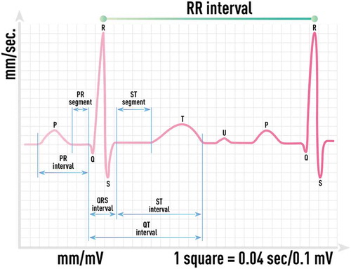
HRV analysis offers a set of measures that are sensitive to such non-obvious changes in heart rate dynamics and can provide complementary insight into cardiac diagnostics [15–17,61,66–69]. HRV sensitivity to non-cardiac abnormalities, emotions, and other complex psycho-physiological states makes it also possible to use HRV analysis beyond the detection of pure cardiac abnormalities. For example, HRV indicators could be used in determining the severity of neurological insult (brain damage) and a prognosis for recovery [74], in understanding neurobiology of psychiatric disorders [75], monitoring of diabetic patients [76], and an easy-to-use and sensitive measure of overtraining in athletes [77], and in monitoring of driver alertness and other changes in psycho-physiological state [78].

The most advanced analytical indicators used in HRV analysis are based on NLD-inspired complexity measures (e.g. DFA, MSE and multifractal extensions) and advanced linear indicators including spectral (frequency-domain) measures. Detrended fluctuation analysis (DFA) was proven to be useful in revealing the extent of long-range correlations in time series. First, the investigated time series of length N is integrated. Next, the integrated time series is divided into n boxes of equal length. In each box, a least-square line is fit to the data with y coordinate denoted by y_n(k) (representing the trend in that box). Finally, the integrated time series, y(k), is de-trended as follows:

(5) $F(n)=\sqrt{\frac{1}{N}\sum _{k=1}^N{\left[y(k)-y_n(k)\right]}^2}$(5)

A linear relationship on the plot of log F(n) vs. log n indicates a power law (fractal) scaling characterized by a scaling exponent β (slope of the fitted straight line). Peng et al. found that F(n) computed from RR time series is characterized by two scaling exponents β₁ and β₂ (cross-over phenomena) computed over a smaller (4 < n < 16) interval and a larger (16 < n < 64) interval, respectively [66]. The two scaling exponents are computed over approximately 2-hour segments (8 × 10³ beats) and presented in Figure 5 of ref [66]. It was shown that the two scaling exponents provide distinctive clustering of the normal and pathological (CHF) cases, however, with noticeable overlapping.

Figure 5. Schematic of error surfaces of low (left panel) and high (right panel) complexity corresponding to problems of low and high dimensionality, respectively. The error function in the high-dimensional space becomes more complex with increasing number of hard-to-avoid local minima.

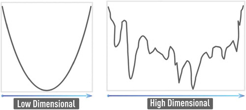
The multiscale entropy (MSE) method [61,67] has been introduced to resolve limitations of traditional single-scale entropy measures. First, a coarse-graining process is applied to the original time series, x_i. Multiple coarse-grained time series are constructed by averaging the data points within non-overlapping windows of increasing length, τ:

(6) $y_j^{(\tau )}=\frac{1}{\tau }\sum _{i=(j-1)\tau +1}^{j\tau }{x}_i$(6)

where τ represents the scale factor and j = 1…N/τ. The length of the coarse-grained time series is N/τ. Next, entropy is calculated for each time series and plotted as a function of the scale factor. A preferable entropy measure is sample entropy (SE) [61,67].

Typical types of MSE behavior have been summarized in Figure 5 of ref [67]. For healthy subjects, the entropy measure increases on small-time scales and then stabilizes to a relatively constant value. Entropy, for subjects with CHF, markedly decreases on small-time scales and then gradually increases for longer time scales. The entropy measure for RR time series, derived from subjects with atrial fibrillation, monotonically decreases. Different features of the MSE curves could be used for separation of normal and pathological cases. One of the simplest features is the slope β₁ of the MSE curve for small-time scales (e.g. between scale factors 1 and 5) [67]. However, although these features could provide statistically significant separation between different classes, the required long duration (~2–4 hours) and significant overlapping of the classes pose the same practical problems as with DFA measures.

In many practical applications, the ability to calculate HRV on short segments of RR data is critical [11–14]. Our analysis indicates that the well-known stylized facts of DFA and MSE measures persist even for significantly shorter RR time series (down to ~5–15 min). However, their abilities for discrimination between healthy and pathological cases could dramatically deteriorate. The same is true for advanced linear measures.

2.1. Universal indicators for robust detection of complex, asymptomatic, emerging and transient cardiac abnormalities

The hybrid boosting-based framework described earlier is generic and is applicable in many different fields. Here we discuss the application of the boosting-based classification framework to the discovery of robust multi-component HRV indicators (i.e. multi-complexity measures) that are capable of working with short RR time series. A natural choice of base models could be low-complexity base classifiers where each of them uses a small subset of the available measures β. Our empirical analysis indicates practicality and robustness of base classifiers based on just a single measure β_i:

(7) $y=h({\beta }_i[p_i],\gamma )$(7)

Here γ is a threshold level (decision boundary) and p_i is a vector of parameters of the chosen measure. Applying boosting steps (2.1)-(2.5) to a set of such base classifiers with different measures β_i and optimizing over (p_i,γ) at each boosting iteration, we obtain a multi-component meta-classifier (Equation (2.5)).

The well-known NLD indicators applicable for HRV analysis are based on DFA (see Equation (5)) [66], MSE (see Equation (6)) [61,67], and multi-fractal analysis (MFA) including MFA extension of DFA [68]. The comparable performance is also demonstrated by advanced linear indicators based on power spectrum analysis of the RR time series [15,69]. One of the widely used indicators of this type is a power spectrum ratio of the low-frequency band (0.04–0.15Hz) to the high-frequency band (0.4–0.15 Hz). Results presented in this paper are based on indicators derived from the described families of HRV measures. However, our framework is open to any other HRV metric that can offer complementary value in cardiac state differentiation.

In general, HRV measures require long-duration time series for stable calculation [11–14]. However, HRV indicators have to be computed on short segments in order to capture early signs of developing and/or intermittent abnormalities or to detect subtle initial effects of treatment procedures. Otherwise, an indicator computed on a long-duration time series will average out these short-lived effects and will fail to detect them. Unlike traditional HRV measures, the proposed ensemble-based indicators are suitable for short-duration, highly sampled, RR time series [11–14].

In all calculations presented in this section, the full data sets, described above, are used. The training data set for ensemble learning algorithms include no more than 50% of normal, CHF, and arrhythmia data combined. LTAF data have not being used in the training phase. Since base classifiers are low-complexity with a small number of adjustable parameters, we have not observed any significant differences between in-sample and out-of-sample results. Further significant reduction of the training data set without performance deterioration is also possible. The number of boosting iterations applied in the considered examples is 30, although the main effects are already captured in 10–20 iterations. Typically, the best-on-average single HRV indicators, which are also picked up at the 1st boosting iteration, are DFA and power spectrum ratio, while MSE is a very important complementary component in the final ensemble and could be important in differentiation of abnormality types.

Performance comparison of typical ensemble classifier with each of single HRV measures in the context of normal/abnormal classification is demonstrated in Figure 19. Since all measures are computed on short RR segments of 256 beats, this analysis relates to an express test when only a short-duration ECG time series is available. However, in cases of emerging and transient abnormalities, the ability to work with short-duration segments is very important, even when long-duration time series (e.g. collected by Holter monitor) are available. As evident from Figure 19, ensemble-based indicator shows significant improvement in all three cases [79].

Figure 19. Detection (i.e. true positive) rates of CHF, LTAF, and arrhythmia for different false alarm (i.e. false positive) rates. All presented measures are computed on short RR segments of 256 beats which is relevant for express diagnostics or monitoring when only a short-duration ECG time series is available. Ensemble-based indicator shows significant improvement over single measures in all three cases of different abnormalities.

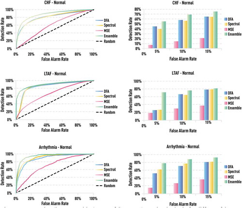
2.2. Rare psycho-physiological states and pathologies: robust detection and quantitative description

Even though the boosting-based approach could significantly improve the accuracy of the normal-abnormal classifier, without re-training, such an indicator may not be able to differentiate between abnormality types [13], as illustrated in Figure 20. Here, the left panel depicts good normal-abnormal classification for both CHF and arrhythmia. On the other hand, the receiver operating characteristic (ROC) curve of the same indicator for CHF vs arrhythmia classification, shown on the right panel, is just slightly better than random. ROC curve is a performance measurement for classification problem at various thresholds settings where ROC curve of the random model without any differentiation ability corresponds to the diagonal line. However, besides aggregated value, the ensemble classifier also offers an EDL vector that implicitly encodes many different regimes/states. By choosing a single reference RR segment (and its EDL vector) from arrhythmia sample (as in the single-example learning approach) and computing distances from this vector to all EDL vectors of arrhythmia and CHF samples, one can obtain the ROC curve for an arrhythmia-CHF classification based on EDL metrics (see Figure 20).

Figure 20. Receiver operating characteristic (ROC) curves of the ensemble indicator. Left: ROC curves of the aggregated ensemble-based indicator. Right: ROC curves based on EDL metrics of the same indicator using full ensemble (green) and MSE-only subset (dashed green). EDL-based ROC curve is significantly better than that based on the aggregated value. By choosing certain sub-components of the ensemble (e.g. only MSE), one can further improve differentiation based on EDL metrics.

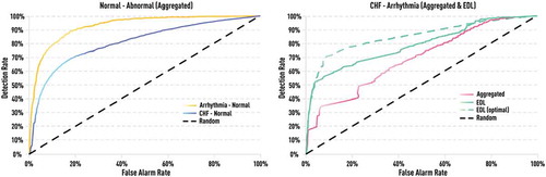
We see that the EDL-based ROC curve is significantly better than that based on the aggregated value. By choosing certain sub-components of the ensemble (e.g. only MSE), one can further improve differentiation based on EDL metrics. In a more generic context, this demonstrates SEL capabilities of EDL-based approach that can be used for the analysis of rare and/or complex abnormalities, where all standard approaches fail due to data limitation [13].

2.3. Generic ensemble-based representation of global cardiovascular dynamics for personalized treatment discovery and optimization

A proper representation of global cardio dynamics could be used for quick and objective matching of the current patient to former cases with known treatment plans and outcomes. Direct comparison of full ECG (RR) time series from two individuals is not effective due to the high level of noise and natural long-term variations of the ECG time series. Collection of consecutive EDL vectors provides effectively filtered representation using natural discretization (classification framework) that removes unimportant variations but preserves differentiation among key micro-states [79]. By calculating Euclidean distances between each EDL vector of one subject with each EDL vector of another subject, the distance matrix is obtained. However, we need the single-number distance measure between two subjects that aggregates comparisons between all of these micro-states represented by EDL vectors. Large distance matrix could be noisy by itself, and usage of simple averages or medians from all cross-EDL distances is not optimal as illustrated later in this section.

The described challenge of handling the distance matrix is similar to that encountered in financial applications dealing with quantification of the market state using large and noisy correlation matrices of thousands of stocks. It was shown that graph-based approaches such as Minimum Spanning Tree (MST) could offer significant advantages over the more traditional approaches based on random matrix theory [80]. MST representation is motivated by the human perception, which organizes information having the most economical encoding. A spanning tree is a connected graph containing all vertices of the original graph without loops [81]. The spanning tree length is defined as the sum of the weights of its edges. MST is a spanning tree with a minimal length among all spanning trees connecting the nodes of the graph. MST of the graph can be derived from Prim’s or Kruskal’s algorithms [81].

Representing long RR time series with a collection of consecutive EDL vectors and using MST for computing aggregated distance between such collections, one can obtain differentiation even within the same abnormality type as illustrated in Figure 21 [79]. Here we show MST-based distances between each pair of 20 CHF patients using a collection of 50 consecutive EDL vectors obtained from the same normal-abnormal ensemble indicator as in Figure 19. We see that the distance of the subject to himself is either minimal or close to minimal. Therefore, since our representation can be used for self-identification, it is natural to assume that other subjects, close to the considered patient in terms of our metrics, have very similar cardiac conditions and responses to personalized treatments.

Figure 21. MST-based distances between each pair of 20 CHF patients using a collection of 50 consecutive EDL vectors computed on 256-beat RR segments. For each subject, distances to all other subjects are represented by black circles. Distance to his own portion of RR time series, not overlapping with the original one, is shown by a red circle. Distance of the subject to himself is either minimal or close to minimal.

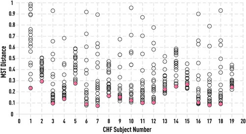
The importance of (1) using ensemble measures, (2) MST for handling cross-subject distance metrics, and (3) long-duration ECG time series, is demonstrated in Figure 22 [79]. Here, we rank the distance of each CHF subject to himself against distances to other subjects. Minimal distance corresponds to rank 1, next after minimal to rank 2, etc. In the case of ideal self-identification, all ranking numbers would be 1.

Figure 22. Rank of the MST-based distance of each healthy, CHF, and LTAF subject to himself against distances to other subjects within the same group. Rank 1 corresponds to minimal distance. Ensemble-based rank (green) is compared to those based on single measures: DFA (blue) and LFHF (yellow). Ensemble-based measure provides a significantly more accurate ranking compared to any single measure.

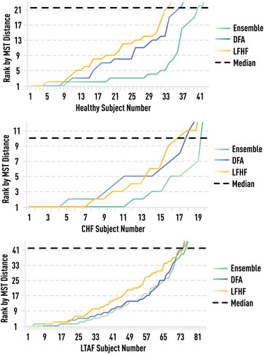
While presented illustrations support the utility of our boosting-based multi-complexity metrics (combined with MST-based aggregation) for fine-grain characterization of the personal cardiac state, the ultimate test of our metrics would consist of identification of subjects with close cardiac states before treatment and establishing whether the same specialized treatments produce similar outcomes. While we are still in the process of collecting such detailed test data, results of the application of our overall framework to real clinical data are very encouraging [79].

2.4. Model-based generation of realistic ECG time series for the enhancement of machine learning and hybrid systems

As already mentioned, data augmentation using synthetic data obtained from realistic physics-based simulations can be effectively used to compensate lack or scarcity of the real data for rare patterns/regimes in biomedical applications. Such synthetic data can be very useful in the pre-training phase of DNN-based DL frameworks as well as in other supervised training algorithms including boosting. Often, even when detailed simulations based on fundamental physical equations are possible, much more useful are coarse-grained proxy models with just a few macro components and parameters characterizing living system state ranging from normal (healthy) to different stages and types of abnormality.

In the context of cardiovascular applications, one such simplified model based on the system of ordinary differential equations (ODE) was proposed in [58] and schematically illustrated in Figure 23. This physiologically motivated, dynamical model of cardiovascular autonomic regulation was shown to be capable of generating heart rate (RR) time series with long-range correlations and multifractal properties very similar to those observed in real RR data [58]. This model consists of a system of delay-differential equations based on the one proposed by Seidel and Herzel and later modified by Kotani et al. [58] to incorporate additional factors needed to simulate synchronization between heartbeat and respiration. In short, this model captures several main physiological factors including: (a) neural afferents from blood pressure sensors (i.e. baroreceptors) to the central nervous system; (b) autonomic sympathetic and parasympathetic neural efferents from the brain stem cardiovascular centers; (c) mechanical signal transduction within the cardiovascular system finally setting the arterial blood pressures; and (d) the effect of the baroreceptor afferents on the instantaneous phase of the respiratory oscillator [58].

Figure 23. Schematic diagram of the cardiovascular/respiratory model proposed in [58]. The diversity in the model is caused mainly by factors such as time delays in the neural conduction, multiplications in neural and mechanical variables, and time-varying Windkessel dynamics. The model consists of a system of delay-differential equations.

The model has several parameters characterizing baroreceptor activity, the efferent sympathetic neural activity, parasympathetic neural activity, etc. [58]. By varying these parameters one can generate any number of synthetic RR time series for a wide range of normal and abnormal conditions, including those rare and/or complex states that are not available in any databases of real cardiac data. Therefore, real cardiac data can be augmented with these synthetic data for significant enhancement of DNN-based DL (in both pre-training and supervised training stages) and boosting-based multi-complexity approaches.

3. Gait time series analysis for diagnostics and monitoring of neurodegenerative diseases

Variability metrics of gait stride intervals are known to be sensitive to changes in neurological functions associated with aging and development of certain neurological diseases [74–77]. Long-range correlation and other measures of stride-interval dynamics could be effective in detecting neurological abnormalities and in the quantification of their severity [74–77]. These include Parkinson’s (PD) and Huntington’s (HD) diseases, amyotrophic lateral sclerosis (ALS), and others.

The remaining challenges in treatment and diagnostics of ALS, PD, HD, and other neurological abnormalities maintain the field’s significant interest in unobtrusive modalities capable of early diagnostics and robust monitoring of such abnormalities. Therefore, variability indicators computed from stride-interval time series could provide a convenient and robust tool for early diagnostics and monitoring of neurological abnormalities. A generic set of NLD complexity measures and linear indicators used in HRV analysis can be directly applied to gait quantification after recalibration.

However, similar to HRV analysis, the accuracy of NLD measures and advanced linear indicators could significantly deteriorate when applied to shorter-duration segments of gait time series [20]. Nevertheless, the combination of complementary complexity measures using boosting-like algorithms can significantly increase the accuracy and stability of indicators operating on short segments of gait time series. Such multi-complexity measures could be effective for early detection and monitoring of a wide range of neurological abnormalities. We provide a short summary of results reported in our previous publications [20].

To illustrate the capabilities of our ensemble-based indicator, we use gait data collected from normal subjects and patients with ALS, HD, and PD that are available at http://www.physionet.org. We use segment durations as short as 128 stride intervals for calculation of DFA, MSE and power spectrum measures that were used as base classifiers in AdaBoost framework. Since low-complexity base classifiers are used, we do not find any significant signs of overfitting on out-of-sample data. In the following, performance metrics are computed on all available data. The classifier from the first boosting iteration is the best single classifier. In our case, it always happens to be a DFA-based classifier.

Figures 24 and 25 illustrate that, although the best single indicator computed on short gait time series is still capable to provide some differentiation between normal and abnormal states, boosting-based combination drastically increases the detection rate (by 40–50%) for reasonable false alarm rates.

Figure 24. Single DFA measure computed on each of 128-interval segments of stride data from the normal control group and patient groups with ALS, HD, and PD (left panel). Aggregated ensemble measure computed on each of 128-interval segments of stride data from the normal control group and patient groups with ALS, HD, and PD (right panel). Although the best single indicator computed on short gait time series is still capable to provide some differentiation between normal and abnormal states, boosting-based combination significantly improves such differentiation.

Figure 25. Abnormality detection rates for a given false alarm rate: The best single measure vs ensemble of multi-complexity measures. Although the best single indicator computed on short gait time series is still capable to provide some differentiation between normal and abnormal states, boosting-based combination drastically increases the detection rate (by 40–50%) for reasonable false alarm rates.

4. Subtle psycho-physiological states differentiation based on ECG, gait and other physiological time series

Besides pure medical applications, variability analysis of physiological time series could be also used for detection and monitoring of psychological conditions and abnormalities. For example, anxiety disorders, chronic stress conditions, depression, and other psychological abnormalities are often associated with the reduction of HRV [82 and references therein]. HRV is known as an objective impact measure of the mainstream and alternative (e.g. meditation) therapies in applied psychology [82 and references therein]. Gait is also known to be a potential indicator of depression, autistic-spectrum disorders, and other psychological and psychiatric conditions [82 and references therein]. Since modern wearable technology (e.g. fitness wearable devices and smartphone sensors) can be easily used for convenient collection of data required for HRV and gait variability calculation, variability indicators could provide very efficient means of continuous monitoring of psychophysiological state and early detection of developing abnormalities. This could also be used for objective assessment of the therapy impact and its subsequent optimization.

It turns out that our ensemble-based HRV indicators could be effectively used in detecting general changes in psychophysiological states [82]. This capability is illustrated in Figure 26, where psychophysiological states before and during Chi meditation are quantified (data from http://www.physionet.org are used). Our ensemble-based measure clearly shows the expected improvement of the psychophysiological state, quantified by HRV metrics, in meditation compared to the pre-meditation period. Overall, single HRV indicators also indicate the correct direction. However, there is significant overlapping between pre-meditation and meditation states, which indicates excessive noise compared to any ensemble-based measure. This could make the distinction between two states much less reliable. Similarly, the ensemble-based measure could be much more robust in early detection of subtle changes in psychological conditions and in their monitoring for an objective choice of optimal therapy and its further fine-tuning [82].

Figure 26. 10-th percentile of the distribution of ensemble (left panel) and single indicators (two right panels) computed on the consecutive 256-beat RR segments of 1 hour Holter monitor recordings before (green) and during (blue) Chi meditation for 7 subjects. Ensemble-based measure clearly shows the expected improvement of the psychophysiological state in meditation compared to the pre-meditation period. Although single measures also indicate the correct direction, there is significant overlapping between pre-meditation and meditation states.

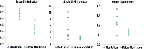
While we are not aware of any large open-access databases capturing slow development of neurological abnormalities, other gait databases can be used for illustration of slow physiological regime changes that can be captured by gait time-series analysis. One of them is the gait maturation database, first analyzed by Hausdorff et al. [83] and now available at http://www.physionet.org. The gait-maturation database is a collection of gait time series from 50 children of various age groups: from 3 to 14 years old. For each subject, a time series is up to 500 stride intervals long. It is known that in very young children, immature control of posture and gait results in unsteady locomotion. In children 3 years old, gait appears relatively mature. However, as suggested in [83], the dynamics of walking changes continues beyond this age. This was confirmed by quantitative analysis of 50 children from the gait-maturity database [84]. Single time- and frequency-domain measures as well as DFA-based measures have been used in that study. It was demonstrated that, while gait in younger age groups resembles that of adults with neurological abnormality, it continuously matures and approaches the dynamical range of healthy young adults as age increases. Hausdorff et al. [84] calculated the indicators using significantly long-duration segments (at least 256 stride intervals), and there was still a wide overlap of indicator values among different age groups. Such overlap could only increase for shorter segments.

This overlap is not critical for the main objective of the analysis presented in [84]. However, for early detection of any slow regime change due to developing abnormality or initial treatment effects, insufficient discrimination capabilities of single indicators could make them useless in practice. Thus, gait maturation database offers convenient real-life data to demonstrate the advantages of our ensemble measures. For this purpose, we compare the best single indicator (DFA) and ensemble-based metrics discovered in the normal/abnormal classification scope.

We applied these indicators to short (128-interval) segments from different age groups and summarized the results as box plots in Figure 27, which demonstrates that a single DFA indicator is not capable to detect any clear trend in gait dynamics with respect to the short-intervals evolution as child age increases. On the other hand, the multi-complexity ensemble indicator shows a clear trend towards gait dynamics of healthy adults as age increases.

Figure 27. Single DFA measure computed on each of 128-interval segments of stride data from three different age groups of healthy subjects (upper panel). Aggregated ensemble measure computed on each of 128-interval segments of stride data from three different age groups of healthy subjects (bottom panel). A single DFA indicator is not capable to detect any clear trend in gait dynamics with respect to the short-intervals evolution as child age increases, while the multi-complexity ensemble indicator shows a clear trend towards gait dynamics of healthy adults as age increases.

V. Summary

Limitations of modern machine learning approaches caused by training-data incompleteness have been reviewed. Hybrid learning framework that leverages existing domain-expert knowledge, including physics-based models, boosting-like model combination, DNN-based DL, and other machine learning algorithms for drastic reduction of training-data requirements have been proposed. Application of the framework to physiological data analysis is illustrated using real data from http://www.physionet.org. Utility of the proposed synergetic combination of physics-based reasoning and machine learning to other biomedical applications has also been discussed.

Acknowledgments

This work was supported in part by the Grant of President of Russian Federation for young scientists No. MK-1896.2017.9 (contract No. 14.W01.17.1896-MK)

Disclosure statement

Authors claim no potential conflict of interest exists.

References

- Toga AW, Kuttler KG, Simpson KJ, et al. Automated detection of physiologic deterioration in hospitalized patients. J Am Med Inform Assoc. 2015 Nov;22:204–256.
- Denaxas SC, Morley KI. Big biomedical data and cardiovascular disease research: opportunities and challenges. Eur Heart J - Qual Care Clinl Outcomes. 2015 July 1;1:9–16.
- Cano A. A survey on graphic processing unit computing for large-scale data mining. WIREs Data Min Knowl Discovery. 2018;8:e1232.
- Grover P, Kar AK. Big data analytics: a review on theoretical contributions and tools used in literature. J Flex Syst Manag. 2017;18:203.
- LeCun Y, Bengio Y, Hinton G. Deep learning. Nature. 2015 May;521:436–444.
- Deng L, Yu D. Deep learning: methods and applications. Found Trends Signal Process. 2014 June;7:197–387.
- Friedman J. Machine. Ann Stat. 2001 Oct;29:1189–1232.
- Chen T, Guestrin C. XGBoost: a scalable tree boosting system. Proceedings of the 22Nd ACM SIGKDD International Conference on Knowledge Discovery and Data Mining; 2016 August 13-17 San Francisco, CA, USA. p. 785–794.
- Bishop CM. Pattern recognition and machine learning. New York, NY: Springer-Verlag; 2006.
- Gavrishchaka VV. Boosting-based frameworks in financial modeling: application to symbolic volatility forecasting. In: Fomby TB, Terrell D, editors. Econometric analysis of financial and economic time series advances in econometrics. Vol. 20, part 2. Bingley, UK: Emerald Group Publishing Limited; 2006. p. 123–151.
- Gavrishchaka VV, Koepke ME, Ulyanova ON. Ensemble learning frameworks for the discovery of multi-component quantitative models in biomedical applications. Proc ICCMS. 2010;4:329–336.
- Gavrishchaka VV, Senyukova OV. Robust algorithmic detection of cardiac pathologies from short periods of RR data. In: Pham TD, Jaim LC, editors. Knowledge-based systems in biomedicine and computational life science, studies in computational intelligence. Vol. 450. Heidelberg, Germany: Springer; 2013. p. 137–153.
- Senyukova OV, Gavrishchaka VV. Ensemble decomposition learning for optimal utilization of implicitly encoded knowledge in biomedical applications. Proc Comput Intell Bioinf. 4, 2011. 69–73.
- Senyukova O, Gavrishchaka V, Koepke M. Universal multi-complexity measures for physiological state quantification in intelligent diagnostics and monitoring systems. In: Pham TD, Ichikawa K, Oyama-Higa M, et al., editors. Biomedical informatics and technology, ACBIT 2013, communications in computer and information science. Vol. 404. Berlin, Germany: Springer-Verlag Berlin; 2014. p. 76–90.
- Voss A, Schulz S, Schroederet R, et al. Methods derived from nonlinear dynamics for analysing heart rate variability. Phylosophical Trans Royal Soc A. 2009 Jan;367:277–296.
- Belair J, Glass L, An der Haiden U, et al. Dynamical disease: mathematical analysis of human illness. New York: AIP Press; 1995.
- Kantz H, Schreiber T. Nonlinear time series analysis. Cambridge UK Cambridge University Press; 1997.
- Schapire RE. The design and analysis of efficient learning algorithms [Ph.D. dissertation]. MA: Massachusetts Institute of Technology Cambridge; 1992.
- Friedman J, Hastie T, Tibshirani R. Additive logistic regression: a statistical view of boosting (With discussion and a rejoinder by the authors). Ann Stat. 2000 Apr;28:337–407.
- Gavrishchaka V, Senyukova O, Davis K. Multi-complexity ensemble measures for gait time series analysis: application to diagnostics, monitoring and biometrics. In: Sun C, Bednardz T, Pham TD, et al., editors. Advances in experimental medicine and biology. Vol. 823. Cham, Switzerland: Springer International Publishing; 2015. p. 107–126.
- Hinton GE, Salakhutdinov RR. Reducing the dimensionality of data with neural networks. Science. 2006 July;313:504–507.
- Gehring J, Miao Y, Metze F, et al. Extracting deep bottleneck features using stacked auto-encoders. International Conference on Acoustics, Speech, and Signal Processing; 2013 May 26-30 Vancouver,p. 3377–3381.
- Gavrishchaka V, Yang Z, Miao R, et al. Advantages of hybrid deep learning frameworks in applications with limited data. Int J Mach Learn Comput. 2018;8:549–558.
- Che Z, Purushotham S, Khemain R, et al. Distilling knowledge from deep networks with applications to healthcare domain. arXiv:151203542 [statML]. 2015 Dec 11.
- Zhou Z-H, Feng J. Deep forest: towards an alternative to deep neural networks. Proceedings of the Twenty-Sixth International Joint Conference on Artificial Intelligence; 2017 August 19-25 Melbourne, p. 3553–3559.
- Filonenko E, Seeram E. Big data: the next era of informatics and data science in medical imaging: a literature review. J Clin Exp Radiol. 2018;1:1.
- Ågren R. On metabolic networks and multi-omics integration [PhD Thesis, Department of Chemical and Biological Engineering, Chalmers University of Technology, Gothenburg, Sweden]; 2013
- Grimbs S. Towards structure and dynamics of metabolic networks [PhD Thesis, University of Potsdam]; 2009
- Saha1 R, Chowdhury A, Maranas CD. Recent advances in the reconstruction of metabolic models and integration of omics data. Curr Opin Biotechnol. 2014;29:39–45.
- Hastie T, Tibshirani R, Friedman J. The elements of statistical learning, Springer Series in Statistics. New York, NY: Springer New York Inc; 2001.
- Fiete IR. Learning and coding in biological neural networks [PhD Thesis]. Cambridge, MA: Harvard University; 2003
- Aljadeff J, Lansdell BJ, Fairhall AL, Kleinfeld D, 2016, Analysis of Neuronal Spike Trains, Deconstructed, Neuron. 91, pp. 221-59. doi: 10.1016/j.neuron.2016.05.039.
- Kohonen T. Self-organization and associative memory. New York: Springer; 1989.
- Rumelhart DE, Hinton GE, Williams RJ. Learning representations by back-propagating errors. Nature. 1986 Oct;323:533–536.
- Werbos PJ. Backpropagation through time: what it does and how to do it. Proc IEEE. 1990 Oct;78:1550–1560.
- Hochreiter S, Schmidhuber J. Long short-term memory. Neural Comput. 1997 Nov;9(8):1735–1780.
- Kolmogorov, AN, On the representation of continuous functions of many variables by superposition of continuous functions of one variable and addition, 1957, Dokl. Akad. Nauk SSSR, 114, 953–956.
- Cybenko G. Approximation by superpositions of a sigmoidal function. Math Control Signals Syst. 1989 Dec;2:303–314.
- Saxe AM, McClelland JL, Ganguli S. Exact solutions to the nonlinear dynamics of learning in deep linear neural networks. arXiv:13126120v3 [csNE]. 2014 Feb 19.
- Dziak JJ, Coffman DL, Lanza ST, Li R. 2017. Sensitivity and specificity of information criteria. PeerJ Preprints 5:e1103v3 https://doi.org/10.7287/peerj.preprints.1103v3.
- Vapnik V. The nature of statistical learning theory. Heidelberg: Springer Verlag; 1995.
- Vapnik V. Statistical learning theory. New York: Wiley; 1998.
- Ratsch G. Robust boosting via convex optimization: theory and applications [Ph.D. thesis, University of Potsdam] ; 2001
- Scholkopf B, Tsuda K, Vert JP, Eds. Kernel methods in computational biology (computational molecular biology). Cambridge, MA: MIT Press; 2004.
- Gavrishchaka VV. BOOSTING-BASED FRAMEWORK FOR PORTFOLIO STRATEGY DISCOVERY AND OPTIMIZATION. New Math Nat Comput. 2006;2:315.
- Freund Y, Schapire RE. A decision-theoretic generalization of on-line learning and an application to boosting. J Comput Syst Sci. 1997;55:119.
- Valiant LG. A theory of the learnable. Commun ACM. 1984;27:1134.
- Elder JF IV. The generalization paradox of ensembles. J Comput Graph Stat. 2003;12:853–864.
- Krizhevsky A, Sutskever I, Hinton GE. Imagenet classification with deep convolutional neural networks. In: Pereira F, Burges CJC, Bottou L, et al., editors. NIPS'12 Proceedings of the 25th International Conference on Neural Information Processing Systems; 2012 December 03-06; Lake Tahoe, Nevada; 2012 p. 1097–1105.
- Banerjee S, Gavrishchaka VV. Multimoment convecting flux tube model of the polar wind system with return current and microprocesses. J Atmos Sol Terr Phys. 2007 Nov;69:2071–2080.
- Erhan D, Bengio Y, Courville A, Manzagol P-A, Vincent P, Bengio S, Why Does Unsupervised Pre-training Help Deep Learning? Journal of Machine Learning Research 11 (2010) 625-660.
- Shin H, Roth HR, Gao M, et al. Deep convolutional neural networks for computer-aided detection: CNN architectures, dataset characteristics and transfer learning. IEEE Trans Med Image. 2016 May;35:1285–1298.
- Christodoulidis S, Anthimopoulos M, Ebner L, et al. Multisource transfer learning with convolutional neural networks for lung pattern analysis. IEEE J Biomed Health Inform. 2017 Jan;21:76–84.
- Huang Z, Pan Z, Lei B. Transfer learning with deep convolutional neural network for SAR target classification with limited labeled data. Remote Sens. 2017 Aug;9:907.
- Bart E, Ullman S. Single-example learning of novel classes using representation by similarity. Proceedings of the British Machine Vision Conference; 2005 September 5-8; Oxford Brookes University, Oxford.
- Horton W, Doxas I. A low-dimensional energy-conserving state space model for substorm dynamics. J Geophys Res (Space Phys). 1996;101:27223–27237.
- Gavrishchaka VV, Ganguli SB. Optimization of the neural-network geomagnetic model for forecasting large-amplitude substorm events. J Geophys Res. 2001;106:6247–6257.
- Kotani K, Struzik ZR, Takamasu K, et al. Model for complex heart rate dynamics in health and diseases. Phys Rev E. 2005;72:041904.
- Gavrishchaka VV, Ganguli SB. Volatility forecasting from multiscale and high-dimensional market data. Neurocomputing. 2003;55(1–2):285–305.
- Gavrishchaka VV, Banerjee S. Support vector machine as an efficient framework for stock market volatility forecasting. Comput Manage Sci. 2006;3:147–160.
- Costa M, Goldberger A, Peng C-K. Multiscale entropy analysis of biological signals. Phys Rev E. 2005;71:021906.
- Ramanna R, Tchalekian R. Simulation: a must for autonomous driving, NVIDIA’s GPU Technology Conference; 2018 (GTC), Washington, DC; Talk ID: S8859.
- Goodfellow IJ, Pouget-Abadie J, Mirza M, Xu B, Warde-Farley D, Ozair S, Courville A, Bengio Y. Generative adversarial nets. NIPS'14 Proceedings of the 27th International Conference on Neural Information Processing Systems; 2014 December 8-13; Montreal, Canada; 2. p. 2672-2680.
- Aliper A, Plis S, Artemov A, et al. Deep learning applications for predicting pharmacological properties of drugs and drug repurposing using transcriptomic data. Mol Pharmaceutics. 2016;13:2524−2530.
- Kadurin A, Aliper A, Kazennov A, et al. The cornucopia of meaningful leads: applying deep adversarial autoencoders for new molecule development in oncology. Oncotarget. 2017;8(7):10883–10890.
- Peng C-K, Havlin S, Stanley EH, et al. Quantification of scaling exponents and crossover phenomena in nonstationary heartbeat time series. Chaos. 1995 Sep;5:82–87.
- Costa M, Goldberger AL, Peng C-K. Multiscale entropy analysis of biological signals. Phys Rev Lett E. 2005 Feb;71:021906.
- Makowiec D, Dudkowska A, Zwierz M, Gałąska R, Rynkiewicz A (2006), Scale Invariant Properties in Heart Rate Signals, Acta Phys Pol B. 37:1627–1639.
- Task Force of the European Society of Cardiology the North American Society of Pacing Electrophysiology. Heart rate variability: standards of measurement, physiological interpretation, and clinical use. Circulation. 1996 Mar;93:1043–1065.
- Hausdorff JM, Mitchell SL, Firtion R, et al. Altered fractal dynamics of gait: reduced stride-interval correlations with aging and Huntington’s disease. J Appl Physiol. 1997;82:262–269.
- Hausdorff JM, Lertratanakul A, Cudkowicz ME, et al. Dynamic markers of altered gait rhythm in amyotrophic lateral sclerosis. J Appl Physiol. 2000;88:2045–2053.
- Damouras S, Chang MD, Sejdic E, et al. An empirical examination of detrended fluctuation analysis for gait data. Gait Posture. 2010;31:336–340.
- Ota L, Uchitomi H, Suzuki K, Hove MJ, Orimo S, Miyake Y. Relationship between fractal property of gait cycle and severity of Parkinson’s disease. in IEEE/SICE International Symposium on System Intergration; 2011 December; Kyoto, Japan.
- Biswas AK, Scott WA, Sommerauer JF, et al. Heart rate variability after acute traumatic brain injury in children. Crit Care Med. 2000;28:3907–3912.
- Yang AC, Hong CJ, Tsai SJ, Heart rate variability in psychiatric disorders, Taiwanese Journal ofPsychiatry 24, 99-109 (2010).
- Akinici A, Celiker A, Baykal E, et al. Heart rate variability in diabetic children: sensitivity of the time- and frequency-domain methods. Pediatr Cardiol. 1993;14:140–146.
- Baumert M, Brechtel L, Lock J, et al. Heart rate variability, blood pressure variability, and baroreflex sensitivity in overtrained athletes. Clin J Sport Med. 2006;16:412.
- Smrcka P, Bittner R, Vysoky P, Hána K, Fractal and multifractal properties of heartbeat interval series in extremal states of the human organism, Measurement Science Review 3, 13–15 (2003).
- Senyukova O, Gavrishchaka V, Sasonko M, et al. Generic ensemble-based representation of global cardiovascular dynamics for personalized treatment discovery and optimization. In: Nguen NT, Iliadis L, Manolopoulos Y, et al., editors. Computational collective intelligence: 8th International Conference on Computational Collective Intelligence ICCCI, 2016 September 28-30; Halkidiki, Greece 9875; p. 197–207.
- Onnela J-P, Chakraborti A, Kaski K, et al. Dynamics of market correlations: taxonomy and portfolio analysis. Phys Rev E. 2003;68:056110.
- Theodoridis S, Koutroumbas K. Pattern recognition. San Diego, CA: Academic Press; 1998.
- Senyukova O, Gavrishchaka V, Tulnova K. Multi-expert evolving system for objective psychophysiological monitoring and fast discovery of effective personalized therapies. Proceedings of IEEE Conference on Evolving Adaptive Intelligence Systems; 2017; Ljubljana, Slovenia;p. 1–8.
- Hausdorff J, Zemany L, Peng C, et al. Maturation of gait dynamics: stride-to-stride variability and its temporal organization in children. J Appl Physiol. 1999;86:1040–1047.
- Hausdorff J, Lertratanakul A, Cudkowicz ME, et al. Dynamic markers of altered gait rhythm in amyotrophic lateral sclerosis. J Appl Physiol. 2000;88:2045–2053.