Advances in multi-dimensional super-resolution nonlinear optical microscopy

ABSTRACT

In this review, recent advances toward bridging the mismatching length scales of optical spectroscopy and imaging are described. Spectroscopic measurements that span ultraviolet to infrared wavelengths provide rich details about the structural properties of molecules and materials. However, the diffraction limit precludes the spatial resolution needed to image these systems commensurate with structure. Many groups have innovated statistical approaches that allow an optical point source to be determined, or ‘localized,’ with a precision that approaches the molecular length scale. As we review here, interferometric nonlinear optical imaging (INLO) allows researchers to simultaneously acquire spectroscopic data and localize the point source in three dimensions with nanometer precision using a single wide-field microscope. Employing plasmonic nanoparticles as prototypical systems, we show that INLO yields sample excitation spectrum, coherence lifetimes (i.e. homogeneous linewidth), and polarization-dependent responses. The INLO method can also be used for polarization-resolved (e.g. circular dichroism) imaging. Hence, multiple dimensions of spectroscopic information content can be added to the optical image. A discussion of prospects for extending the INLO-localization platform to other so-called super-resolution spectroscopy measurements is also provided.

GRAPHICAL ABSTRACT

KEYWORDS:

• Super-resolution
• ultrafast microscopy
• nonlinear optics
• imaging
• plasmonics

I. Introduction

Throughout nature, chemical and physical properties are determined by subtle, structural effects that span the Ångstrom to micron length scales. Some examples include the Ångstrom-level influences of inter-nuclear separation on molecular energy levels and the relative arrangement of nanoparticles on a few-to-tens of nanometer lengths on inter-particle modes. Insight into these types of structure-property correlations can often be inferred from optical spectroscopy measurements. However, the diffraction limit of light typically restricts the spatial resolution of these measurements to a few hundred nanometers (resolution ≈ λ/2), precluding the direct spatial correlation of these relationships. Many strategies to overcome the intrinsic spatial limitations of optical imaging have been demonstrated [1–5]. One approach that can be carried out in a conventional wide-field microscope is based on the statistical localization of a signal point source[6]. Although this method can yield spatial precisions on the order of one nanometer [3,7], it lacks much of the information content that optical spectroscopy measurements can provide. Hence, there is a need for an imaging method that can combine the spatial precision attainable from statistical localization with the information afforded by optical spectroscopy.

Our group has approached this problem – the incompatibility of optical imaging and spectroscopy length scales – by developing interferometric nonlinear optical imaging methods that utilize phase-stable laser pulses and array detection [8–12]. Statistical localization of the signal point spread function obtained from an imaging array yields information about position, while Fourier analysis of the interferometrically collected data provides spectroscopic outputs. Here, we review this work and illustrate how the interferometric approach can yield polarization, phase, time, and frequency information – all while preserving the nanometer precisions of spatial localization methods. In a recent advance, we showed that the axial (out-of-plane) position of the point source can also be determined with high (≈ 20 nm) spatial precision[13]. A major challenge to achieving high spatial resolution with simultaneous time and phase information is preserving the positional stability of the sample and laser pulses in the interaction region during the data acquisition time. A method for achieving high stability in all of the necessary experimental parameters to acquire these data is described in this review.

Specific examples are drawn from our work on plasmonic nanoparticles and assemblies. Nanoscale materials offer many opportunities to use and control energy. One prominent example is the localized surface plasmon resonance (LSPR), which is a characteristic feature of colloidal nanoparticles typically formed from precious metals, resulting from coherent electronic excitation of conduction band electrons [14–16]. LSPR excitation is responsible for amplification of many light-harvesting applications such as surface-enhanced spectroscopy [17–20], photocatalysis [21,22], molecular sensing [23–25], and selective spatial localization of light to nanoscale volumes [26–28]. LSPR excitation can also form the basis for nonlinear optical switching and provide the functional basis for nonlinear metasurfaces[12]. These applications can be substantially enhanced when LSPR-supporting nanoparticles are organized into a network, forming collective inter-particle resonances [29–32]. However, the resonance frequencies and light-harvesting properties of these inter-particle plasmon modes are extremely sensitive to the precise nanoscale arrangement of these particles, as well as to particle-to-particle heterogeneity [33–36]. Therefore, in order to achieve predictive photonic function from plasmonic and other nanoparticle assemblies, direct structure-optical correlations must be made.

The remainder of this review is organized as follows: the experimental methods of interferometric nonlinear optical imaging are described in Section II; a theoretical description of the two-dimensional statistical localization framework is described in Section III; lateral (2D) localization is demonstrated using experimental results in Section IV; extension of the Sections II through IV framework to three-dimensional localization is given in Section V; specific examples where polarization, frequency- and time-domain information was obtained by using femtosecond interferometric imaging are given in Section VI; and concluding remarks and outlooks for future research directions are provided in Section VII.

II. Experimental methods: nonlinear optical imaging

The experimental setup for nonlinear optical microscopy has been described in detail previously [7–11]. Figure 1 provides the optical layout for nonlinear optical (NLO) measurements. A mode-locked Ti:Sapphire oscillator (center wavelength = 800 nm; pulse duration ≈ 10 fs; repetition rate = 55 MHz) was focused to the sample plane of a home-built microscope, and used as the fundamental excitation source for NLO measurements. The NLO signal was collected through a microscope objective (100x, oil immersion, NA = 1.25) and focused to the entrance slit of a spectrometer connected to an electron multiplying charge coupled device (EMCCD, Andor Technology). The size of the pixels in the EMCCD array are 144 ± 3 nm, which allows point-source localization on the nanometer length scale (described in Sections III & IV). This setup can be configured with different polarizers, waveplates, and optical filters to generate many different imaging modalities. NLO signals are isolated for detection using a series of notch and bandpass filters. The NLO measurements are correlative with bright-field and dark-field imaging, as well as electron microscopy[7]. A broadband white light source (SPL-2 H, Photon Control Inc.) was used for bright-field and dark-field imaging.

Figure 1. Optical layout used for multi-dimensional interferometric nonlinear optical (INLO) imaging. Components include: PRG: Pulse Replica Generator, λ/2: half-wave plate; ASL: aspherical lens; S: sample; Obj.: compound objective (100x, NA = 1.25)

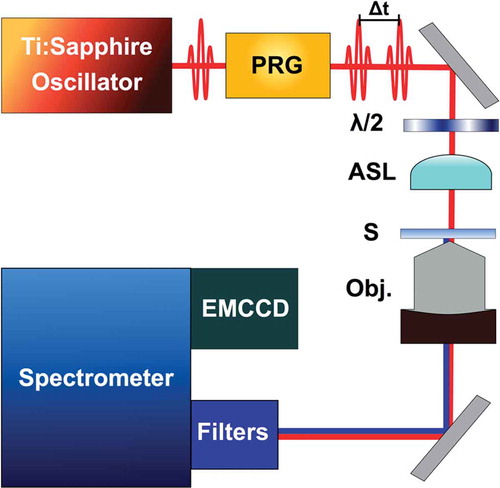
A key advance that allows time-domain and polarization-resolved interferometry measurements is the generation of phase-locked pulse replicas that propagate collinearly. This collinear beam geometry provides facile incorporation into a home-built optical microscope. The pulse replicas are generated using a method referred to as Translating Wedge-based Identical pulse eNcoding System (TWINS) technology [11,37]. An important advantage of this method is that the inter-pulse time delay separating the replicas can be adjusted for pulses projected in either parallel or perpendicular planes. Interferometry using pulses aligned in a parallel plane provides time (and frequency) domain analysis of the sample’s resonance response. Interferometry using orthogonally projected pulses, delayed on the sub-cycle time scale, allows the polarization state of the fundamental to be systematically varied. We note that for 800-nm light, circular polarization is achieved when a time delay of 667 attoseconds is applied to two orthogonal pulses. As described in Section V, we routinely achieve sub-15 attosecond inter-pulse phase stability, which is persistent for longer than two hours and more than sufficient to acquire circular dichroism (CD) images.⁹ Depending on the type of measurement, image frame exposure times vary from milliseconds to seconds.

III. Statistical framework for two-dimensional (transverse) localization

The problem of the diffraction limit is illustrated in Figure 2. Figure 2(a) is a wide-field image of the second harmonic light generated from dimeric gold nanoparticle assemblies arranged in a grid following interaction with femtosecond laser pulse. Each white spot in the image was obtained from a single, isolated nanoparticle dimer. Due to the diffraction limit of light, the individual nanoparticle components that form the dimer assembly were not resolvable; instead, the assemblies appear as a single blurred out spot (i.e. a point-spread function (PSF). Figure 2(b) is a scanning electron microscope image of a grid of nanoparticle dimers, clearly resolving the individual nanoparticles making up the assemblies. Although both images are limited by diffraction, the resolution of the electron microscope is much finer, owing to the shorter de Broglie wavelength of the accelerated electrons. Nevertheless, the location of the emission point source can be determined with very high precision using statistical localization methods, which are based on centroiding the experimentally measured PSF.

Figure 2. The diffraction limit for optical and electron microscopy. (a) Diffraction-limited nonlinear optical (NLO) second harmonic generation (SHG) image of an array of nanoparticle assemblies. (b) Scanning electron microscope image of an array of nanoparticle assemblies. The scale bars in both (a) and (b) represent 2 μm. Panels (a) and (b) illustrate the resolution problem caused by the diffraction limit. In (a), the individual components of the assemblies are unresolvable and appear as a single spot with a width of ~500 nm. In contrast, in the SEM image (b), the individual components are clearly resolvable. Localization imaging techniques allows for the determination of the position of a signal point source with much higher precision than the optical diffraction limit

The precision with which one can use statistical centroiding methods to determine the location of an optical point source is quantified by the following equation derived by Thompson et. al [6].

(1) $pre=\sqrt{\frac{{\sigma }^2}{N}+\frac{a^2}{12N}+\frac{8\pi {\sigma }^4{b}^2}{a^2{N}^2}}$(1)

Where pre is the localization precision in determining the point spread function (PSF) centroid, σ is the standard deviation determined from fitting the point spread function to a 2-D Gaussian function, a is the image pixel size, b is the standard deviation of the background, and N is the number of detected photons.

The achievable precision in determining the location of a point source is directly proportional to the noise in the optical system. There are two limiting cases to consider: (1) when the noise is dominated by the shot noise of photon detection and (2) when the noise is dominated by background counts (e.g. out-of-focus light, CCD readout noise, dark noise, etc.). The effects of these two types of noise on the achievable precision will be examined individually, then an overall equation for the precision will be derived.

First, the photon-noise limited case is considered. Each photon collected in an image provides a measure of the position of an object. The position error from each measurement is given by the standard deviation of the point spread function (PSF), σ. Figure 3(a) depicts a 2-D Gaussian distribution of 10,000 simulated photons from an emitter positioned at (0,0) in the (x,y) plane of a 3-D coordinate frame; the laser propagation and signal collection are along the z axis. The standard deviation of the PSF in this simulated microscope was 150 nm. To estimate the position of an object, the positions of the detected photons were averaged. The uncertainty in this measurement is quantified by the standard error of the mean, given by

(2) $⟨{\left(\mathrm{\Delta }x\right)}^2⟩=\frac{{\sigma }^2}{N}$(2)

Figure 3. Simulated photon distributions. (a) 2-D Gaussian distribution of detected photons from an object positioned at (0,0) in the (x,y) plane of a 3-D coordinate frame. The standard deviation of the simulated PSF was 150 nm. Each point represents the location a single photon (10,000 total). (b) Binned data from (a) with a bin width of 144 nm to illustrate the additional uncertainty introduced by the finite size of pixels that compose the CCD sensor

where σ is the standard deviation of the point spread function, and N is the number of detected photons. Equation 2(2) $⟨{\left(\mathrm{\Delta }x\right)}^2⟩=\frac{{\sigma }^2}{N}$(2) yields the uncertainty in determining the position of an object in the photon- noise limited case. However, to this point, we have assumed that the exact position of each individual photon can be determined with infinite precision, which is not possible due to finite size of the CCD pixels. The exact position of each photon cannot be determined beyond the bin size of one pixel, which induces further uncertainty in the determination of an object’s position. This pixilation noise is illustrated in Figure 3(b). The data in Figure 3(a) has been binned into finite pixels, and the uncertainty of the location of the emitter measurement has increased. This pixilation uncertainty can be calculated as the variance of a uniform distribution of size a, the image pixel width. Using the formula for variance – $Var(x)=⟨x^2⟩-{⟨x⟩}^2$; where $⟨x⟩={\int }_0^{a}x(1/a)dx=a/2$ and $⟨x^2⟩={\int }_0^a{x}^2(1/a)dx=a^2/3$ for a uniform distribution from 0 to a – the pixilation uncertainty can be calculated as a²/12. Adding this uncertainty in quadrature to the photon shot noise from Equation 1(1) $pre=\sqrt{\frac{{\sigma }^2}{N}+\frac{a^2}{12N}+\frac{8\pi {\sigma }^4{b}^2}{a^2{N}^2}}$(1) , we arrive at Equation 3(3) $⟨{\left(\mathrm{\Delta }x\right)}^2⟩=\frac{{\sigma }^2}{N}+\frac{a^2}{12N}$(3) .

(3) $⟨{\left(\mathrm{\Delta }x\right)}^2⟩=\frac{{\sigma }^2}{N}+\frac{a^2}{12N}$(3)

Equation 3(3) $⟨{\left(\mathrm{\Delta }x\right)}^2⟩=\frac{{\sigma }^2}{N}+\frac{a^2}{12N}$(3) provides the positional uncertainty or precision of determining the location of an object when the photon shot noise limits the precision.

All detected photons do not necessarily originate from the emitting object; there can be contributions from many background sources – such as out-of-focus light, CCD readout noise, and dark noise – in the recorded image. Background noise is included in determination of localization precision using Chi-square statistics to estimate the error associated with fitting experimental data to expected theoretical values. For simplicity, we will begin by considering localization in one dimension. The sum of squared errors, χ²(x), between the observed photon count at pixel i, y_i, and the expected photon count, N_i(x), of a PSF located at x is given by

(4) ${\chi }^2(x)=\sum _i\frac{{(y_i-N_i(x))}^2}{{{\xi }_i}^2}$(4)

where ξ_i is the expected photon count uncertainty at pixel i and is the sum of uncertainties due to photon-counting noise and background noise b. ξ_i is expressed as

(5) ${{\xi }_i}^2=N_i(x)+b^2$(5)

where the variance of the photon-counting noise is equal to the expected number of photons, N_i(x), and b is the standard deviation of the background noise. Equation 4(4) ${\chi }^2(x)=\sum _i\frac{{(y_i-N_i(x))}^2}{{{\xi }_i}^2}$(4) is minimized by setting it’s derivative equal to zero.

(6) $\frac{d{\chi }^2}{dx}=\sum _i\left[\frac{{(y_i-N_i(x))}^2}{{{\xi }_i}^2}\frac{d}{dx}\right]=0$(6)

Equation 6(6) $\frac{d{\chi }^2}{dx}=\sum _i\left[\frac{{(y_i-N_i(x))}^2}{{{\xi }_i}^2}\frac{d}{dx}\right]=0$(6) is simplified to Equation 7(7) $\sum _i\frac{-2(\mathrm{\Delta }{y}_i+{N_i}^{\mathrm{\prime }}\mathrm{\Delta }x)(-N_i)}{{{\xi }_i}^2}=\sum _i\frac{{(\mathrm{\Delta }{y}_i+{N_i}^{\mathrm{\prime }}\mathrm{\Delta }x)}^2(2N_i)}{{{\xi }_i}^4}$(7) by expanding N_i(x) around the actual particle position, x₀, and collecting first order terms where Δx=x–x₀.

(7) $\sum _i\frac{-2(\mathrm{\Delta }{y}_i+{N_i}^{\mathrm{\prime }}\mathrm{\Delta }x)(-N_i)}{{{\xi }_i}^2}=\sum _i\frac{{(\mathrm{\Delta }{y}_i+{N_i}^{\mathrm{\prime }}\mathrm{\Delta }x)}^2(2N_i)}{{{\xi }_i}^4}$(7)

Where N_i′ is the derivative of N_i evaluated at x₀ and Δy_i= N_i(x₀) – y_i. Solving Equation 7(7) $\sum _i\frac{-2(\mathrm{\Delta }{y}_i+{N_i}^{\mathrm{\prime }}\mathrm{\Delta }x)(-N_i)}{{{\xi }_i}^2}=\sum _i\frac{{(\mathrm{\Delta }{y}_i+{N_i}^{\mathrm{\prime }}\mathrm{\Delta }x)}^2(2N_i)}{{{\xi }_i}^4}$(7) for Δx yields Equation 8(8) $\mathrm{\Delta }x=-\frac{\sum _i\frac{\mathrm{\Delta }{y}_i{N}_i(x{)}^{\prime }}{{\xi }_i^2}\left(1-\frac{\mathrm{\Delta }{y}_i}{2{\xi }_i^2}\right)}{\sum _i\begin{array}{c}\frac{{\left(N_i(x{)}^{\prime }\right)}^2}{{\xi }_i^2}\end{array}\left(\begin{array}{c}\frac{1-\mathrm{\Delta }{y}_i}{{\xi }_i^2}\end{array}\right)}$(8) , which – assuming relatively small errors in counted photons – becomes Equation 9(9) $\approx -\frac{\sum _i\begin{array}{c}\frac{\mathrm{\Delta }{y}_i{N}_i(x{)}^{\prime }}{{\xi }_i^2}\end{array}}{\sum _i\begin{array}{c}\frac{{\left(N_i(x{)}^{\prime }\right)}^2}{{\xi }_i^2}\end{array}}$(9) .

(8) $\mathrm{\Delta }x=-\frac{\sum _i\frac{\mathrm{\Delta }{y}_i{N}_i(x{)}^{\prime }}{{\xi }_i^2}\left(1-\frac{\mathrm{\Delta }{y}_i}{2{\xi }_i^2}\right)}{\sum _i\begin{array}{c}\frac{{\left(N_i(x{)}^{\prime }\right)}^2}{{\xi }_i^2}\end{array}\left(\begin{array}{c}\frac{1-\mathrm{\Delta }{y}_i}{{\xi }_i^2}\end{array}\right)}$(8)

(9) $\approx -\frac{\sum _i\begin{array}{c}\frac{\mathrm{\Delta }{y}_i{N}_i(x{)}^{\prime }}{{\xi }_i^2}\end{array}}{\sum _i\begin{array}{c}\frac{{\left(N_i(x{)}^{\prime }\right)}^2}{{\xi }_i^2}\end{array}}$(9)

The mean square error of the position measurement can be calculated by squaring Equation 9(9) $\approx -\frac{\sum _i\begin{array}{c}\frac{\mathrm{\Delta }{y}_i{N}_i(x{)}^{\prime }}{{\xi }_i^2}\end{array}}{\sum _i\begin{array}{c}\frac{{\left(N_i(x{)}^{\prime }\right)}^2}{{\xi }_i^2}\end{array}}$(9) and taking the expectation value to produce Equation 10(10) $⟨{\left(\mathrm{\Delta }x\right)}^2⟩=\frac{1}{\sum _i\frac{{\left({N_i}^{\mathrm{\prime }}\right)}^2}{{\xi }_i^2}}$(10) ,

(10) $⟨{\left(\mathrm{\Delta }x\right)}^2⟩=\frac{1}{\sum _i\frac{{\left({N_i}^{\mathrm{\prime }}\right)}^2}{{\xi }_i^2}}$(10)

which, when evaluated, estimates the uncertainty of the position measurement. Equation 10(10) $⟨{\left(\mathrm{\Delta }x\right)}^2⟩=\frac{1}{\sum _i\frac{{\left({N_i}^{\mathrm{\prime }}\right)}^2}{{\xi }_i^2}}$(10) can be evaluated by approximating N_i with

(11) $N_i=\frac{N{a}^2}{\sigma \sqrt{2\pi }}exp\left(-\frac{{\left(ia\right)}^2}{2{\sigma }^2}\right)$(11)

and replacing the summation in Equation 9(9) $\approx -\frac{\sum _i\begin{array}{c}\frac{\mathrm{\Delta }{y}_i{N}_i(x{)}^{\prime }}{{\xi }_i^2}\end{array}}{\sum _i\begin{array}{c}\frac{{\left(N_i(x{)}^{\prime }\right)}^2}{{\xi }_i^2}\end{array}}$(9) with an integral where i is continuous from negative to positive infinity. There are two limits of approximation; one being the high photon count limit (ξ_i [2] = N_i) and the other being the high background noise limit (ξ_i [2] = b [2]). In the high photon count limit, the integral simplifies to Equation 2(2) $⟨{\left(\mathrm{\Delta }x\right)}^2⟩=\frac{{\sigma }^2}{N}$(2) . For the case of high background noise,

(12) $⟨{\left(\mathrm{\Delta }x\right)}^2⟩=\frac{4\sqrt{\pi }{\sigma }^3{b}^2}{a{N}^2}$(12)

To this point, we have considered localization in one dimension. To expand to two dimensions, the previous equations span two indices (i and j), yielding a two-dimensional integral in the approximation of Equation 9(9) $\approx -\frac{\sum _i\begin{array}{c}\frac{\mathrm{\Delta }{y}_i{N}_i(x{)}^{\prime }}{{\xi }_i^2}\end{array}}{\sum _i\begin{array}{c}\frac{{\left(N_i(x{)}^{\prime }\right)}^2}{{\xi }_i^2}\end{array}}$(9) . The result for calculating the uncertainty in the high background noise regime in the 2-D case is

(13) $⟨{\left(\mathrm{\Delta }x\right)}^2⟩=\frac{8\pi {\sigma }^4{b}^2}{a^2{N}^2}$(13)

The expressions for uncertainties evaluated in the limiting cases discussed (photon counting noise, pixilation noise, and background noise) can be combined into one equation by adding the uncertainties in quadrature to produce Equation 13(13) $⟨{\left(\mathrm{\Delta }x\right)}^2⟩=\frac{8\pi {\sigma }^4{b}^2}{a^2{N}^2}$(13)

(14) $⟨{\left(\mathrm{\Delta }x\right)}^2⟩=\frac{{\sigma }^2}{N}+\frac{a^2}{12N}+\frac{8\pi s^4{b}^2}{a^2{N}^2}$(14)

which, upon taking the square root, transforms into Equation 1(1) $pre=\sqrt{\frac{{\sigma }^2}{N}+\frac{a^2}{12N}+\frac{8\pi {\sigma }^4{b}^2}{a^2{N}^2}}$(1) – the precision in determining the location of an emitter.

IV. Experimental demonstrations of lateral (2D) localization

The location of the signal point source is determined by analyzing NLO images using the statistical methods described in Section III. Data was analyzed with a home-written script in Igor Pro. First, the NLO images are fit to a 2-D Gaussian function to determine the standard deviation, σ. The number of NLO photons, N, was the sum of photons from all pixels falling under the 2-D Gaussian fit. The image pixel size, a, was calibrated by imaging a TEM grid and determined to be 144 ± 3 nm[7]. The standard deviation of the background, b, was determined by collecting a background image and calculating the standard deviation of the pixel photon values in the region of interest. Figure 4(a) shows a SHG image obtained from a heterotrimer composed of three solid gold nanospheres of cascading sizes. The 2-D Gaussian fit to this data is overlaid in Figure 4 panel (b).

Figure 4. Representation of the NLO super-resolution imaging technique. (a) A SHG image record from a gold nanosphere heterotrimer. Scale bar = 500 nm. (b) Raw SHG data from (a) overlaid with the results from PSF fitting with a 2-D Gaussian. (c) A representative electron microscopy image of a gold nanoparticle heterotrimer overlaid with the localization imaging results as 1-σ (blue) and 2-σ (red) confidence regions. Scale bar represents 100 nm. Adapted with permission from reference 28

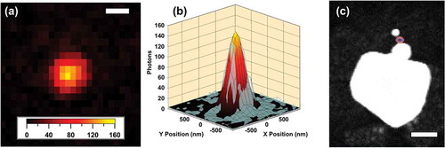
The specific location of NLO emission within nanoparticle assemblies was determined by correlating the optical results with electron microscopy images. This correlation method has been described previously in detail[7]. Briefly, a patterned microscope cover slip is used in conjunction with neighboring nanoparticle assemblies acting as fiduciary markers to ensure unique pattern matching for correlation between optical and electron microscopies. After assemblies are imaged with both optical and electron microscopy, the localization data are overlaid as concentric ellipses that correspond to 1-σ and 2-σ confidence levels by adjusting the scaling the of images and using the fiducial markers as guides. An overlay of the optical localization results and the SEM image of the solid gold nanosphere (SGN) heterotrimer is presented in Figure 4(c). The 1-σ localization precision confidence level was 7 nm (blue ring). The second harmonic generation (SHG) signal was localized to the inter-particle gap between the two smallest nanospheres. This data demonstrates the ability of statistical localization of diffraction-limited optical images collected in the far field to pinpoint signals within the near field of a nanoparticle network.

Electromagnetic energy confinement in gold nanosphere assemblies

In this section, we describe the use of resonantly enhanced NLO imaging to determine the electromagnetic energy-confining regions of gold nanosphere assemblies with nanometer spatial precision. The largest impact on spatial precision, determined by Equation 1(1) $pre=\sqrt{\frac{{\sigma }^2}{N}+\frac{a^2}{12N}+\frac{8\pi {\sigma }^4{b}^2}{a^2{N}^2}}$(1) , is the number of detected photons. This poses a problem for collecting images of objects involving NLO signals, as they are typically weak and limit the localization accuracy. However, this can be overcome by using plasmonic nanoparticles to act as electromagnetic antennas and to increase the optical signal strength resulting from the NLO process[7]. This signal enhancement offers two important benefits for nanoparticle imaging with high spatial precision: (1) plasmon amplification of the NLO signal significantly increases the precision with which a point source can be localized, and (2) the image contrast results from nanostructure mode-specific responses due to selective excitation of inter-particle plasmon resonances.

To demonstrate mode-selective plasmon imaging, the effects of plasmon amplification on localization accuracies were studied by acquiring SHG images using different fundamental energies and polarizations[7]. The intensity of SHG generated from plasmonic nanoparticles has a strong dependence on energy matching between the fundamental wave and the plasmon resonance. This can be understood by considering the second-order polarizability of the material, which for SHG includes the second-order susceptibility, χ⁽²⁾, approximated as

(15) ${\chi }^{(2)}(\omega )\propto {\chi }^{(1)}(2\omega )\cdot [{\chi }^{(1)}(\omega ){]}^{(2)}$(15)

Where χ⁽¹⁾(2 ω) and χ⁽¹⁾(ω) represents the linear response of the material at the harmonic and fundamental frequencies, respectively[38]. Thus, resonance matching of the nanoparticle plasmon mode to the fundamental frequency can be used to increase the number of detected SHG photon, and hence increase the localization precision. This effect is experimentally demonstrated in Figure 5(a) where the localization precisions from four different SGN dimers are plotted versus the energy difference between the fundamental (800 nm) and the LSPR maximum. The localization precision improved significantly as the energy difference is decreased. In all particles, the optimal localization precision resulted when the difference between the plasmon frequency and the fundamental frequency was minimized. The different localization accuracies determined for each structure reflect the sensitivity of statistical localization to structure-specific inter-particle mode coupling.

Figure 5. Factors that affect localization accuracy. (a) Localization accuracy calculated from four different nanoparticle dimers plotted versus |effective χ⁽²⁾|. As the LSPR and fundamental wave were detuned in energy, large structure-dependent changes were observed. (b) Dependence of localization accuracy on excitation energy and acquisition frame rate. Black dots represent measured localization accuracies, and rainbow surface represents interpolated fits to the data with the localization equation[26]. The plane at z = 3.41 nm marks the localization accuracy with minimum laser detuning and maximal |effective χ⁽²⁾| and fastest frame rate. (c) Polar plot of localization accuracy plotted against the polarization angle formed between the fundamental light source and the inter-particle axis. Reproduced with permission from reference 7

The importance of resonance-energy matching between the laser fundamental and the resonant plasmon mode can also be seen in Figure 5(b). Here, the localization precision is plotted as a function of fundamental energy and imaging frame rate. As the exposure time was increased, the localization accuracy improved for all excitation energies. However, as the fundamental energy was detuned from the LSPR, a point was observed when the localization accuracy approached an asymptote and could no longer be improved with longer image acquisition. The plane at z = 3.41 nm marks the localization precision observed with minimum laser detuning and fastest frame rate. This behavior indicates that the NLO localization method is ultimately noise limited and demonstrates the benefits of resonance matching to enhance plasmon amplification in coupled nanoparticle antennas in order to achieve high spatial accuracy and fast temporal dynamic range.

The mode specificity of localization imaging is further demonstrated in Figure 5(c) with polarization-dependent measurements. For these experiments, the incidence angle between the linearly polarized fundamental wave and the inter-particle axis was altered, using a wave plate/polarizer combination, as NLO images were acquired. A bright plasmon mode was generated when the linearly polarized light was oriented parallel to the inter-particle axis of the electromagnetically coupled nanoparticle dimer[39], and a dark plasmon mode was excited when the light’s electric field was rotated to an orthogonal plane[7]. The localization results in Figure 5(c), obtained over 360° rotation of the incident polarization, clearly demonstrate the mode specificity of single-particle imaging. Excitation of the bright mode resulted in increased SHG yield compared to dark-mode excitation, which resulted in no SHG signal. As the localization precision is highly sensitive to the signal strength, it showed a polarization-dependent, mode-specific response. When the bright mode was excited (Figure 5(c), 0°), the best localization accuracy was achieved. In contrast, when the dark mode was excited (Figure 5(c), 180°), no signal was observed.

Investigating nanoscale light focusing using localization imaging

Figure 6 depicts the application of NLO localization for pinpointing the electromagnetic hotspot position in a light-harvesting plasmonic nanostructure. Gold nanoparticle heterotrimers were constructed as described previously using directed assembly methods [27,28]. The asymmetric trimer was chosen as a model system because the arrangement of progressively smaller nanospheres in a linear configuration is predicted to result in cascaded focusing of light from the large antenna-like nanoparticle to the junction between the two smallest receiver-like nanoparticles[31]. This energy funneling effect is demonstrated in numerically simulated electric field maps in Figure 6(a,b), where the electromagnetic hotspot is localized to the inter-particle gap between the two smallest spheres when the excitation was aligned parallel to the inter-particle axis (a), and the electromagnetic field was largely localized near the larger nanosphere when the excitation was aligned orthogonal to the inter-particle axis (b).

Figure 6. (a,b) Simulated electric field map for a trimer nanolens excited with a fundamental wave polarization aligned parallel (a) and perpendicular (b) to the inter-particle axis. (c,d) Experimental localization using localization imaging with parallel (c) and perpendicular (d) polarization with respect to the inter-particle axis, reported as 1-σ (magenta) and 2-σ (cyan) confidence levels, overlaid with electron microscopy images of the nanoparticle trimer. The scale bar in (d) represents 100 nm. Adapted with permission from reference 28

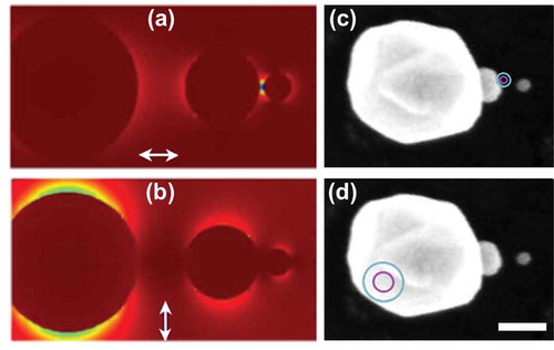
Experimental NLO localization imaging results are provided in Figure 6(c,d) from nanoparticle assemblies consisting of 250-, 80-, and 30-nm diameter nanospheres. The experimental results agree with numerical predictions and confirm that the electromagnetic energy was localized to the inter-particle gap between the two smallest nanospheres with parallel polarization (Figure 6(c)), consistent with electromagnetic confinement within the network. Localization imaging revealed that the experimental SHG signal obtained using orthogonal excitation originated from the larger nanosphere, which indicated that energy focusing and localization through the network did not occur when the excitation source was polarized perpendicular to the inter-particle axis[28]. Traditional diffraction-limited imaging methods could not distinguish these two different responses because the spatially distinct hotspots within the trimer were separated by less than 100 nm. The Figure 6 data demonstrate that the localization imaging method can be used as a tool to examine nanoscale electromagnetic energy transfer and confinement in nanoparticle networks.

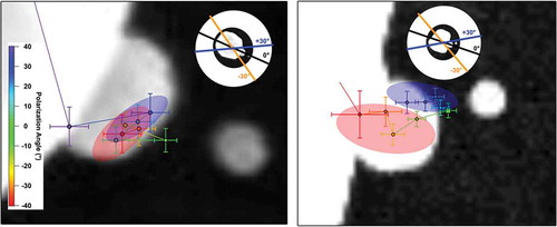
The polarization-dependent location of the SHG emission is further investigated using nonlinear nanolens trimers, as shown in Figure 7. Here, the point source location is plotted at different polarization angles with respect to the inter-particle axis, where 0° indicates that the polarization was parallel to the inter-particle axis formed between the two larger spheres. Localization imaging was performed on an ideal, linear heterotrimer (left panel) and a non-linear trimer where the smallest nanoparticle was shifted off of the interparticle axis. In both cases, we observed that the point source was located between the medium and smallest-sized particles, closer to the middle (medium) particle (green point). As the polarization was rotated away from 0°, the emission location shifted toward the center of mass of the assembly. In the case of the linear assembly (left panel), the point source locations shifted toward the nanostructure center of mass independently of the polarization rotation direction, indicated by overlapping red and blue regions in the figure. In contrast, the movement of the emission location showed a polarization-angle dependent response for the nonlinear trimer case (right panel). This can be observed as a clustering of localization positions near the gap between the two smallest particles (blue region) as the plane of polarization became parallel to the inter-particle axis formed between the smallest particles (≈ +30°). As the polarization was rotated in the opposing direction, the determined point source locations behaved more like the linear trimer case (red region). Taken together, these results demonstrate that localization imaging can be a powerful tool for pinpointing structure-specific and mode-selective signals in nanoparticle networks.

Figure 7. Polarization-dependent localization imaging of an ideal (left) and non-ideal (right) gold nanoparticle trimer. Colored markers represent localization spots determined with NOLES imaging with 1-σ confidence levels as error bars. The color of the marker identifies the incident polarization angle of the fundamental source with respect to the inter-particle axis. The figures in the inset indicate how the polarization angles orient with respect to the full nanoassembly. The red and blue shaded regions indicate where the localization centers clustered at the extremes of the polarization rotation. Adapted with permission from reference 28

V. Axial (3D) localization

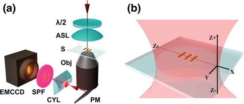
In this section, we describe how diffraction-limited images can be used to obtain sub-diffraction localization precisions in three dimensions. Our approach[13], which we term variable displacement-change point detection (VD-CPD), incorporates a Bayesian online change point detection algorithm that is used to identify differences in the image beam waist that result from small, axial displacements of the sample within the microscope focal plane. The experimental layout of the 3D NLO imaging setup is shown in Figure 8a. This optical setup is similar to the one shown in Figure 1, but includes a cylindrical lens that is used to manipulate the image focus at the detector plane in response to variations in sample position. Specifically, the cylindrical lens introduces an astigmatism in the collected images by creating different focal lengths in the x- and y- axes. One other critical modification to the experimental setup is that the microscope objective is mounted on a closed-loop piezo stage (nPoint Inc., LC 400) that allowed control over sample axial position (position noise of the stage is ±3 nm). Here, we demonstrate the effectiveness of this approach using two-photon photoluminescence signals from gold nanorods.

Figure 8. (a) Optical layout of the NLO microscope. Components included: λ/2: half-wave plate, ASL: aspherical lens, S: sample, Obj.: compound objective lens, PM: plane mirror, CYL: cylindrical lens, SPF: short-pass filter. (b) Illustration of the spatial coordinate axes. The red-dotted line designates the axial position corresponding to the average lateral (X, Y) focal plane, Z₀. Variable axial displacements are made along the z axis. Adapted with permission from reference 13 © The Optical Society

The spatial coordinate system for the imaging experiments is described in Figure 8b. The red dotted line indicates the axial position Z₀, corresponding to the average lateral (x, y) excitation focal plane. Controlled, variable displacements of the sample, with respect to this lateral focus, were made along the z axis. When the sample is located in the average lateral focus, the diffraction-limited image is symmetric in the 2D image plane. However, upon axial sample displacement, the acquired image becomes distorted. This effect can be seen in Figure 9(a-c). In our specific case, an upward axial displacement (away from the cylindrical lens) results in elongation of the image width along the x- direction and reduction along the y direction (Figure 9(a)). In contrast, axial displacement toward the cylindrical lens reduces the x-axis width and increases the y-axis width (Figure 9(c)). The changes in the width are quantified using equation 16(16) $G(x,y)=hexp\left[-2\frac{{(x-x_0)}^2}{w_x^2}-2\frac{{(y-y_0)}^2}{w_y^2}\right]+b$(16) :

(16) $G(x,y)=hexp\left[-2\frac{{(x-x_0)}^2}{w_x^2}-2\frac{{(y-y_0)}^2}{w_y^2}\right]+b$(16)

Figure 9. TPPL images obtained for a single AuNR at various z positions; 600 nm above focal plane (a), average focal plane (b) and 600 nm below focal plane (c); (d) Calibration curve of image widths w_x and w_y obtained as a function of sample position, Z, for single gold nanorods (AuNRs). Each data point represents the average value obtained from 30 scans from the same particle, center energy: 1.55 eV, frame rate: 10fps. The data were fit to a defocusing function (red curve) as described in reference 13

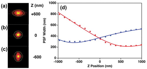
The results from fitting the position-dependent widths using equation 16(16) $G(x,y)=hexp\left[-2\frac{{(x-x_0)}^2}{w_x^2}-2\frac{{(y-y_0)}^2}{w_y^2}\right]+b$(16) are plotted in Figure 9d. The unique crossing point for the w_x and w_y values identifies the average lateral focus[4]. The position of the emitter can be localized with sub-diffraction precision by fitting the Figure 9(d) data using equation 17(17) $w_{x,y}(z)=w_0\sqrt{1+{\left(\frac{z-c}{d}\right)}^2+A{\left(\frac{z-c}{d}\right)}^3+B{\left(\frac{z-c}{d}\right)}^4}$(17) :

(17) $w_{x,y}(z)=w_0\sqrt{1+{\left(\frac{z-c}{d}\right)}^2+A{\left(\frac{z-c}{d}\right)}^3+B{\left(\frac{z-c}{d}\right)}^4}$(17)

Using this method, we obtained an axial localization precision of ≈ 100 nm. This value represents a significant improvement over the several-hundred nanometer out-of-plane diffraction limit for this image. However, this level of positional precision is still insufficient to correlate material structure and optical properties.

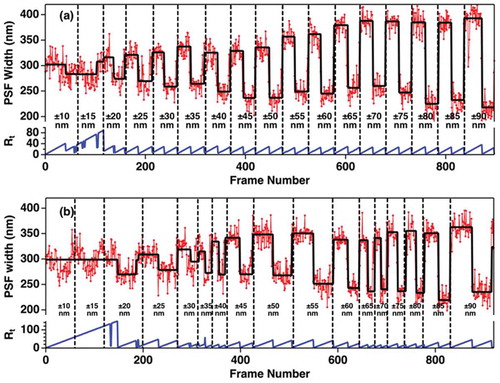
In order to improve the precision of out-of-plane position determinations, we implement the VD-CPD method. Here, we identify the minimal displacement that induces a quantifiable change to w_x, w_y fitting results (equation 17(17) $w_{x,y}(z)=w_0\sqrt{1+{\left(\frac{z-c}{d}\right)}^2+A{\left(\frac{z-c}{d}\right)}^3+B{\left(\frac{z-c}{d}\right)}^4}$(17) ). In order to remove user bias in judging a real change in w_x or w_y, we use a CPD algorithm, as described in reference 13, while introducing axial sample displacements. Figure 10 shows the fitted x and y image point-spread function widths obtained for axial displacement form the average lateral focal plane; displacements spanned the range from ± 10 nm to ± 90 nm. The Figure 10 trajectories clearly show that changes the PSF width can be observed for displacements of only a few tens of nanometers. The effectiveness of the CPD method for quantifying the minimal resolvable displacement is shown in Figure 11. Here, we correlate the PSF w_x values to a specific frame number among a sequence of successively collected frames. The CPD tracks frames yielding similar results as a ‘run.’ When a new w_x value is recorded, the ‘run’ breaks and a new one begins. As the Figure 11 data show, we can reliably resolve displacements of as small as ± 20 nm. Based on these data, the precision in axially locating the sample is improved by ≈ 3x and > 15x compared to astigmatic and diffraction-limited imaging, respectively. Hence, the VP-CPD method provides sub-diffraction spatial precisions.

Figure 10. Position-dependent fitting results for X and Y widths obtained by applying variable z displacement method. The range for the z direction displacement spanned from ±10 nm to ±90 nm. The vertical black lines indicate when the axial, z, position was changed from ±10 nm (left) to ±90 nm (right) in 5 nm increments (center energy: 1.55 eV, 10fps). Adapted with permission from reference 13 © The Optical Society

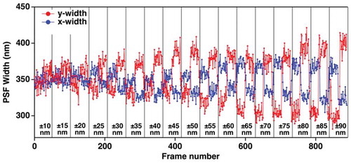
Figure 11. Demonstration of Variable Displacement-Change Point Detection (VD-CPD) analysis method, using (a) constant frame rate of 10 frames/second and (b) variable frame rates. For panel b, the frame rate is randomly varied from 1 frame/second to 10 frames/second. The vertical black lines indicate when the axial, z, position was changed from ±10 nm (left) to ±90 nm (right) in 5 nm increments. Adapted with permission from reference 13 © The Optical Society

VI. Time-domain and polarization-dependent NLO imaging using femtosecond pulse replicas

In this section, we demonstrate the use of interferometric imaging with phase-stable pulse replicas with NLO array detection to obtain spectral, polarization, and time-domain information from resonantly excited samples. In doing so, the information content of so-called ‘super-resolution’ imaging methods can be extended to include spectroscopic results. These interferometric methods can be used in the same imaging platform as was used to obtain the nanoscale spatial precisions described in sections III–V. Polarization-dependent microscopy has been achieved by incorporating TWINS technology into the NLO imaging setup in the form of a Pulse Replica Generator (PRG)[37]. Briefly, phase-locked, collinear laser pulse replicas with a user-controlled inter-pulse time delay are generated using a series of birefringent wedges, grouped in blocks, with optical axes oriented in orthogonal directions, as depicted in Figure 12(a). The polarization of the incoming laser pulse is aligned 45° with respect to the optical axis of block A. After propagation through the material, the parent pulse is split into two orthogonally polarized replicas with a fixed time delay that depends on the thickness of block A. Next, these two pulses propagate through block B, which consists of wedges that, through use of a 1-D translation stage, have a variable thickness. This change of thickness affects the pulse arrival time of one of the two pulses, leaving the other fixed. Block C compensates for the angular dispersion introduced by the wedges in block B. A superposition of the two orthogonal pulses, shifted by sub-cycle temporal delays, can manipulate the polarization state of the laser. For example, inducing a positive (or negative) 667-attosecond inter-pulse delay, one quarter of an optical cycle at 800 nm, can generate left (or right) handed circularly polarized light[9]. This PRG method has been shown to generate pulses with a minimum time step of ~5.7 attoseconds, and is phase stable to ~33 mrad over the course of two hours[9].

Figure 12. Manipulating the polarization state of the fundamental laser source with a pulse replica generator. (a) Schematic depicting the PRG used for polarization manipulation. The legend in the top left indicates orientation of the x-, y-, and z-planes in the figure. The ‘A,’ ‘B,’ and ‘C’ labels designate the three blocks of birefringent materials. Block B is on a motorized translation stage which traverses the x-direction (indicated by the arrow) and induces time delays between two orthogonally polarized phase-locked pulse replicas. The superposition of the two orthogonally polarized components produces circularly polarized light when the time delay is set appropriately. The colors of the wedges in (b) and (c) in indicate the orientation of the optical axis of the birefringent crystal (green: oriented along x-axis, cyan: oriented along y-axis, magenta: oriented along z-axis). Panels (b) and (c) show the retrieved point spread function, constructed form image contrast, for a nanosphere heterotrimer (depicted as SEM inset, scale bar = 100 nm). A clear difference is observed between excitation with left circularly polarized light (b) versus right circularly polarized light (c), indicative of a circular dichroism response. Quantitative analysis revealed a circular dichroism ratio of 1.61 ± 0.16 for this trimer structure. Adapted with permission from references 9 and 28

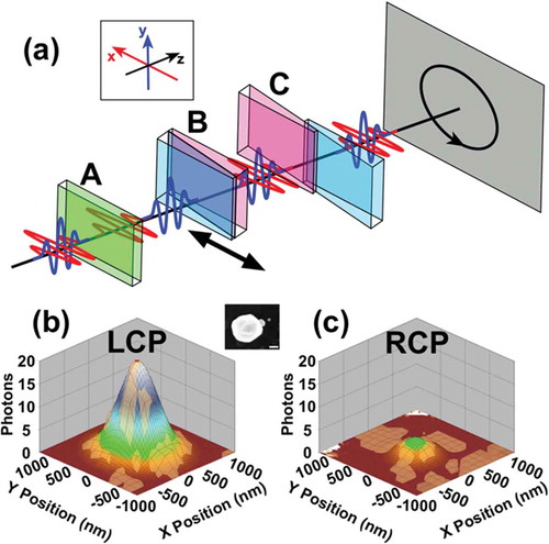
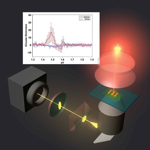
The PRG has been used to generate circularly polarized excitation for SHG-detected circular dichroism imaging[9]. Figure 12(b,c) depicts the SHG signal generated from a trimer nanostructure (SEM image given in inset) upon excitation with left (b) and right (c) circularly polarized light. An unambiguous difference was observed, indicative of preferential absorption of a specific polarization state of light and circular dichroism (CD). The magnitude of the CD response was quantified by the circular difference ratio (CDR), a normalized quantity given as

(18) $CDR=\frac{2(I_{2\omega }^{LCP}-I_{2\omega }^{RCP})}{I_{2\omega }^{LCP}+I_{2\omega }^{RCP}}$(18)

In Equation 18(18) $CDR=\frac{2(I_{2\omega }^{LCP}-I_{2\omega }^{RCP})}{I_{2\omega }^{LCP}+I_{2\omega }^{RCP}}$(18) , I_2ω is the experimentally measured SHG intensity from LCP or RCP excitation from a single GNP nanoassembly. The CDR from the trimer structure yielding the data in Figure 8 was determined to be 1.61 ± 0.16[28].

Coherent electronic relaxation dynamics from interferometric nonlinear optical imaging

In addition to excitation polarization-dependent measurements, the PRG also provides the ability to perform time-resolved, pump-probe measurements on single structures. This time-resolved capability allows for the study of electronic energy relaxation of single structures, which is essential to determine how networks of nanoparticles use electromagnetic energy. For example, plasmon dephasing in metal nanoparticle assemblies influences the achievable optical amplification of the system, where longer coherence times result in greater amplification[8].^,10−12 For time-resolved microscopy, a linear polarizer is inserted after the PRG setup to project the orthogonally polarized components back into a common plane of polarization[8]. Then, the position of the block B wedges can be scanned to create linearly polarized pulse replicas with inter-pulse time delays spanning femtosecond to picosecond time delays. However, a key condition is that the positional stability of the pump and probe pulses must be preserved throughout the entire range of pump-probe time delays used.

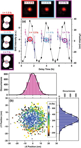
In order to determine the positional stability of our NLO microscope, the localization techniques described in sections III and IV were used to analyze SHG images from a single nanoparticle assembly over a time delay scan of the PRG. Figure 13(a) shows interferometric SHG intensity data (black) at time delays near time zero overlaid with the corresponding x (open magenta circles) and y (open blue circles) relative spatial positions and localization precisions (error bars) determined from localization analysis. These data portray the variation in the measured point source location as a function of inter-pulse delay. The panels at the top of Figure 13(a) are SHG images acquired at the indicated time points circled with matching colors. The panels in the column on the left of Figure 13(a) are SEM images overlaid with localization results at the same time points. At the different time points, the determined hot spot location remained within the gap between the two nanoparticles, and the SHG images are nearly identical, with a variation of less than 10 nm in the point source location. The positional stability was further quantified by analyzing the determined hot spot position over the entire course of a delay scan. Figure 13(b) shows the measured y position versus x position for all delay times (−300 to +750 fs). A cluster of data points centered around (0,0) was observed. The color scale in the image follows the time delay from −300 (black) to +750 fs (blue). Histograms of the position distribution along x and y over an entire delay scan are in the top and left panels, respectively. The histogram data were fit to Gaussian functions, yielding standard deviations of 5.64 ± 0.06 nm in x and 6.74 ± 0.09 nm in y. This result indicates that the positional stability is better than 10 nm over the time delay scan. Altogether, these data demonstrate sufficient spatial localization stability over the experimental time required to acquire femtosecond time-resolved images using our NLO microscope.

Figure 13. Analysis of positional stability of the microscope during a time scan of the inter-pulse delay between phase-locked pulse replicas. (a) Measured SHG image contrast-detected interferogram (black filled circles) overlaid with the measured spatial position (open markers) and localization accuracy (error bars) determined at different time steps along the interferogram. (top) SHG images at time points indicated with color-coded rings and labels. (left) Corresponding SEM images with localization analysis results overlaid, also arranged by color-coded outlines and labels. Scale bar represents 25 nm. (b) Scatter plot of (x, y) centroid positions determined from localization analysis over the temporal range of the interferogram. The histograms report deviations in the x- (top) and y- (right) directions over the entire scan. The histograms were fit with Gaussian distribution functions, which revealed that the position of the point source deviated by less than 10 nm over the entire course of the time-resolved measurements, which is more than sufficient for distinguishing localization points in a nanolens structure. Adapted with permission from reference 7

Next, the ability to resolve electronic relaxation dynamics from plasmonic nanorods with approximate 10-fs time resolution is described. We have demonstrated that interferometric nonlinear optical (INLO) imaging accurately recovers plasmon coherence times using second harmonic (SHG), two-photon photoluminescence (TPPL), and four-wave mixing (FWM) action signals[8].^,10−12 A distinct advantage of the INLO approach over commonly used dark-field scattering (DFS) and transient absorption methods is that the INLO method allows simultaneous determination of the coherence time and nanometer localization of the nonlinear signal point source in 3D, which is not possible using DFS. The combined few-optical-cycle temporal resolution and nanometer-precision that INLO provides will be essential for developing structure-property correlations for complex materials.

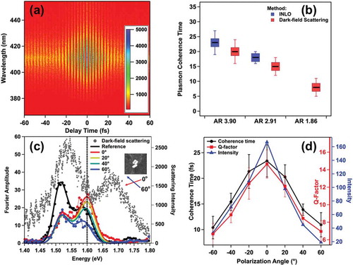
An example of a frequency-resolved, SHG-detected interferogram obtained from a dimeric assembly of gold nanospheres is given in Figure 14(a). The interferogram is generated using a sequence of phase-stabilized femtosecond pulse replicas, which are temporally delayed on the attosecond to femtosecond time scales, as described previously[8]. Whereas polarization-dependent imaging used an orthogonally polarized pulse pair, time-domain measurements are obtained from linearly polarized pulse replicas projected in a common plane. After the non-resonant SHG instrument and sample resonance responses have been determined, time-resolved data resulting from plasmon-resonant excitation of the nanostructure can be extracted (Figure 14(b)). This is accomplished by determining the time-dependent optical response function of a system, R(t), which describes the interaction between a stimulating optical field E(t) and the material. R(t) is modeled as a damped harmonic oscillator in the time domain,

(19) $R(t)=Aexp(i{\omega }_{LSPR}t-\gamma t)$(19)

Figure 14. (a) Representative plasmon-mediated SHG-detected interferogram obtained from plasmonic nanoparticles. Fourier analysis of the interferogram yields the plasmon resonant response, including the homogeneous linewidth. (b) Summary comparison of INLO and DFS- determine plasmon coherence times. The close correspondence of the methods confirms INLO accuracy. (c) INLO and DFS (scatter) comparison for hybridized Dolmen responses. The two methods identify the Fano resonance at 1.6 eV. (d) Comparison of plasmon coherence time and NLO signal intensity

where A gives the effective oscillator strength, ω_LSPR is the plasmon resonance frequency, and γ is the line width described by γ = 1/T₂, where T₂ is the plasmon coherence dephasing time [8,12]. It is important to appreciate that at the single-particle measurement level, γ represents a homogeneous linewidth Γ_h for an electronic, in this case plasmonic, transition and hence, T₂ reports structure- and mode-specific carrier dynamics such as electron-electron, electron-phonon, electron-interband and radiative scattering. The detected polarized output signal is a convolution of the response function and the incident optical field, given by[12]:

(20) $P(t)=\int R(t-t^{\prime })E(t^{\prime })d{t}^{\prime }$(20)

The amplitude and phase of the system response are determined using interferometric frequency-resolved optical gating (IFROG) of the SHG signal to measure

(21) $I_{IFROG}(2\omega ,\tau )\propto |\int {[X(t)+X(t-\tau )]}^{2}exp(-i\omega t)dt{|}^2$(21)

with time delay τ and frequency ω[12]. For a non-resonant nonlinear medium, an instantaneous response proportional to the electric field of the laser fundamental, E(t), gated by the time-delayed pulse E (t − τ), is measured. If the material is resonant within the excitation bandwidth, as is the case for plasmon-resonant excitation, the finite response time leads to an induced polarization transient, and the output signal is a convolution of the driving laser pulse, E(t), and the resonance response function, R(t), given by

(22) $P(t)=E(t)\otimes R(t)=\int R(t-t^{\prime })E(t^{\prime })d{t}^{\prime }.$(22)

R(t), the resonance response function of a system, can be deconvolved from a nonresonant E(t) and P(t) from a resonant plasmonic nanostructure.

The accuracy of INLO methods for capturing plasmon dephasing dynamics is illustrated in Figure 14(b). Here, INLO responses are compared to dark-field linewidth results for single gold nanorods with different nanorod-length-to-diameter aspect-ratios. The three model nanorod systems had AR of 1.86, 2.91, and 3.90, which supported longitudinal LSPR energies of 2.06 eV, 1.77 eV, and 1.55 eV, respectively. The relative contributions of plasmon dephasing processes are volume dependent. Therefore, isolation of structure-specific dynamics requires comparison of constant-volume samples. These studies isolate the influence of interband scattering on plasmon coherence times[10]. Coherent intraband electron scattering with the interband transition is a significant plasmon dephasing mechanism for gold, and rod lengthening allows for energetic decoupling of the plasmon (intraband) excitation from the interband transition. Hence, plasmon coherence times should be extended as the length-to-diameter aspect ratio increases. This effect is clearly identified by INLO Figure 14(b). Good agreement between INLO and DFS, which is a standard method for quantifying plasmon coherence times of nanoparticles, is shown in Figure 14(b). The agreement between the two methods further indicates that the time-dependence of the SHG signals capture the lifetimes of the electronic excitation. Signal amplitudes resulting from decay of surface fields are expected to increase the lifetimes by 2x when compared to the DFS linewidth analysis[12].

The INLO method has also been applied to examine mode-specific dynamics of nanoparticle networks. Here, the objective was to generate inter-particle resonances that mix sub-radiant ‘dark’ modes with optically accessible ‘bright’ modes in order to suppress plasmon radiative decay. One specific example is a ‘dolmen’ assembly of nanorod trimers. The dolmen structure can be treated as two separate but electromagnetically coupled systems: i) a dimer formed by parallel nanorods and ii) a single capping nanorod oriented with its major axis orthogonal to that of the dimer[40]. Excitation that is plane-polarized parallel to the capping nanorod generates sub-radiant multipolar modes in the dimer, which mixes with the radiant longitudinal dipolar resonance of the capping rod forming a Fano resonance. Excitation perpendicular to the capping nanorod results primarily in creation of bright, radiant modes localized to the dimer. Excitation of mixed sub-radiant and radiant modes provides opportunities to extend plasmon coherence times for the nanostructure.

Our experimental results show that the plasmon coherence times for this nanostructure are, indeed, very sensitive to the excitation polarization state. The radiative dark-field scattering spectrum obtained for the Dolmen nanorod trimer is given in Figure 14(c); the specific trimer assembly electron microscope image is shown in the Figure 14(c) inset along with a frame of reference for laser polarization directions. This spectrum shows a region of scattering transparency near 1.6 eV, which reveals the dark-mode Fano-resonance energy. The resonance responses obtained from INLO imaging using several different orientations for the sample-incident-excitation angle are also shown in Figure 14(c). In good agreement with the scattering data, which showed a dip in radiative intensity at this energy, these data clearly reveal an absorptive, polarization-dependent peak at 1.6 eV. The presence of this peak indicates that the dark mode is strongly coupled to instantaneous nanostructure excitation for specific polarizations. The polarization-dependent dephasing times increase from 10 ± 2 fs to 23 ± 3 fs; the persistent coherence times results from dark-mode excitation when the excitation field is polarized parallel to the capping nanorod. The data reflect an approximately 2.3x increase in coherence time when the dark mode is excited. In order to test the hypothesis that preserved coherence increases optical amplification, we have correlated the dolmen two-photon photoluminescence signals to coherence time in Figure 14(d) overlay. These data show a polarization-dependent 9x increase in the intensity of the NLO signal that tracks the coherence time results. These studies demonstrate how interferometric ultrafast NLO imaging, in correlation with electron microscopy, can inform on structure-dependent nanoscale optical properties and carrier dynamics. Because the same array detectors are used in our interferometric measurements and our localization measurements described in Section III, we have the ability to simultaneously correlate coherence and electronic relaxation times to signal position.

VII. Summary and outlook

In this review, we have described a multi-dimensional far-field imaging platform that provides acquisition of signals with high spatial precision, while simultaneously preserving the information content of nonlinear optical spectroscopy. This is accomplished by combining interferometric NLO spectroscopy with array-based image detection. The examples described here included methods for achieving nanometer in-plane (lateral) and tens of nanometers out-of-plane (axial) precisions, along with quantifications of material circular dichroism ratios, excitation spectra and homogeneous linewidths. The latter output also provides electronic dephasing times.

The spectroscopic measurements reviewed here were carried out using one-color, two-pulse interferometry. The inter-pulse time delays spanned the sub-cycle to few-hundred femtosecond range – adequate for characterizing the electronic excitation and coherence dynamics of most materials. The temporal range of the microscope can be easily extended by incorporating an additional delay line, as is used in a typical pump-probe configuration. The use of interferometry in either the pump or probe stages would permit state-resolved excitation or detection, respectively. This experimental advance would give access to state-resolved studies of electronic relaxation dynamics on spatial length scales that are difficult to achieve by other methods. We also note that this approach could enable fifth-order SHG-detected two-dimensional electronic spectroscopy, or SFG imaging with high spatial precisions. To date, most examples of transient-absorption-based ultrafast microscopy are limited to hundreds of nanometers in spatial resolution[41]. Examples of ultrafast microscopy using scanned probe methods do exist, but these measurements are very complex[42]. The combined use of interferometric NLO and array detection offer an attractive approach to achieving high spatial precision and spectroscopic information in a conventional wide-field microscope.

Acknowledgments

This work was supported by grants from the Air Force Office of Scientific Research (FA9550-15-1-0114) and (FA9550-18-1-0347). This work was also supported by awards from the National Science Foundation (CHE-1801829 and CHE-1807999).

Disclosure statement

No potential conflict of interest was reported by the author(s).

Additional information

Funding

This work was supported by the Air Force Office of Scientific Research [FA9550-15-1-0114,FA9550-18-1-0347]; Division of Chemistry [1801829].

References

- Hell SW, Wichmann J. Breaking the diffraction resolution limit by stimulated emission: stimulated-emission-depletion fluorescence microscopy. Optics Letters. 1994;19:780.
- Betzig E, Patterson GH, Sougrat R, et al. Imaging intracellular fluorescent proteins at nanometer resolution. Science. 2006;313:1642.
- Yildiz A, Selvin PR. Fluorescence imaging with one nanometer accuracy: application to molecular motors. Accounts of Chemical Research. 2005;38:574.
- Huang B, Wang W, Bates M, et al. Three-dimensional super-resolution imaging by stochastic optical reconstruction microscopy. Science. 2008;319:810.
- Gustafsson MGL, Shao L, Carlton PM, et al. Three-dimensional resolution doubling in wide-field fluorescence microscopy by structured illumination. Biophysical Journal. 2008;94:4957.
- Thompson RE, Larson DR, Webb WW. Precise nanometer localization analysis for individual fluorescent probes. Biophysical Journal. 2002;82:2775–31.
- Jarrett JW, Chandra M, Knappenberger KL Jr. Optimization of nonlinear optical localization using electromagnetic surface fields (NOLES) imaging. The Journal of Chemical Physics. 2013;138:214202.
- Jarrett JW, Zhao T, Johnson JS, et al. Investigating plasmonic structure-dependent light amplification and electronic dynamics using advances in nonlinear optical microscopy. The Journal of Physical Chemistry C. 2015;119:15779.
- Jarrett JW, Liu X, Nealey PF, et al. Communication: SHG-detected circular dichroism imaging using orthogonal phase-locked laser pulses. The Journal of Chemical Physics. 2015;142:151101.
- Zhao T, Jarrett JW, Johnson JS, et al. Plasmon dephasing in gold nanorods studied using single-nanoparticle interferometric nonlinear optical microscopy. The Journal of Physical Chemistry C. 2016;120:4071–4079.
- Zhao T, Steves M, Chapman BS, et al. Quantification of interface-dependent plasmon quality factors using single-beam nonlinear optical interferometry. Analytical Chemistry. 2018;90:13702–13707.
- Zhao T, Herbert PJ, Zheng H, et al. State-Resolved metal nanoparticle dynamics viewed through the combined lenses of ultrafast and magneto-optical spectroscopies. Accounts of Chemical Research. 2018;51:1433–1442.
- Zhao T, Jarrett JW, Park K, et al. Axial point source localization using variable displacement–change point detection. Journal of the Optical Society of America B. 2018;35:1140–1148.
- El-Sayed MA. Some interesting properties of metals confined in time and nanometer space of different shapes. Accounts of Chemical Research. 2001;34:257.
- Oldenburg SJ, Averitt RD, Westcott SL, et al. Nanoengineering of optical resonances. Chemical Physics Letters. 1998;288:243.
- Gole A, Murphy CJ. Seed-mediated synthesis of gold nanorods: role of the size and nature of the seed. Chemistry of Materials. 2004;16:3633.
- Stiles PL, Dieringer JA, Shah NC, et al. Surface-enhanced raman spectroscopy. Annual Review of Analytical Chemistry. 2008;1:601.
- Jiang N, Foley ET, Klingsporn JM, et al. Observation of multiple vibrational modes in ultrahigh vacuum tip-enhanced Raman spectroscopy combined with molecular-resolution scanning tunneling microscopy. Nano Letters. 2012;12:5061.
- Sivapalan ST, Devetter BM, Yang TK, et al. Off-resonance surface-enhanced Raman spectroscopy from gold nanorod suspensions as a function of aspect ratio: not what we thought. ACS Nano. 2013;7:2099.
- Zhang Y, Zhen YR, Neumann O, et al. Coherent anti-stokes Raman scattering with single-molecule sensitivity using a plasmonic Fano resonance. Nature Communications. 2014;5:4424.
- Zhou X, Andoy NM, Liu G, et al. Quantitative super-resolution imaging uncovers reactivity patterns on single nanocatalysts. Nature Nanotechnology. 2012;7:237.
- Grubisic A, Mukherjee S, Halas N, et al. Anomalously strong electric near-field enhancements at defect sites on Au nanoshells observed by ultrafast scanning photoemission imaging microscopy. The Journal of Physical Chemistry C. 2013;117:22545.
- Gao H, Yang J-C, Lin JY, et al. Using the angle-dependent resonances of molded plasmonic crystals to improve the sensitivities of biosensors. Nano Letters. 2010;10:2549.
- Anker JN, Hall WP, Lyandres O, et al. Biosensing with plasmonic nanosensors. Nature Materials. 2008;7:442.
- Haes AJ, Van Duyne RP. A nanoscale optical biosensor: sensitivity and selectivity of an approach based on the localized surface plasmon resonance spectroscopy of triangular silver nanoparticles. Journal of the American Chemical Society. 2002;124:10596.
- Jarrett JW, Herbert PJ, Dhuey S, et al. Chiral nanostructures studied using polarization-dependent NOLES imaging. The Journal of Physical Chemistry A. 2014;118:8393.
- Biswas S, Liu X, Jarrett JW, et al. Nonlinear chiro-optical amplification by plasmonic nanolens arrays formed via directed assembly of gold nanoparticles. Nano Letters. 2015;15:1836.
- Liu X, Biswas S, Jarrett JW, et al. Deterministic construction of plasmonic heterostructures in well-organized arrays for nanophotonic materials. Advanced Materials. 2015;27:7314.
- Stockman MI, Faleev SV, Bergman DJ. Coherently controlled femtosecond energy localization on nanoscale. Applied Physics B. 2002;74:S63.
- Stockman MI, Faleev SV, Bergman DJ. Coherent control of femtosecond energy localization in nanosystems. Physical Review Letters. 2002;88:67402.
- Li KR, Stockman MI, Bergman DJ. Self-similar chain of metal nanospheres as an efficient nanolens. Physical Review Letters. 2003;91:227402.
- Stockman MI, Faleev SV, Bergman DJ. Femtosecond energy concentration in nanosystems: coherent control. Physica B: Condensed Matter. 2003;338:361.
- Nordlander P, Oubre C, Prodan E, et al. Plasmon hybridization in nanoparticle dimers. Nano Letters. 2004;4:899.
- Hao E, Schatz GC. Electromagnetic fields around silver nanoparticles and dimers. The Journal of Chemical Physics. 2004;120:357.
- Jain PK, El-Sayed MA. Universal scaling of plasmon coupling in metal nanostructures: extension from particle pairs to nanoshells. Nano Letters. 2007;7:2854.
- Nome RA, Guffey MJ, Scherer NF, et al. Plasmonic interactions and optical forces between au bipyramidal nanoparticle dimers. The Journal of Physical Chemistry A. 2009;113:4408.
- Brida D, Manzoni C, Cerullo G. Phase-locked pulses for two-dimensional spectroscopy by a birefringent delay line. Optics Letters. 2012;37:3027.
- Boyd RW. Nonlinear Optics. Second ed. London, United Kingdom: Academic Press; 2003.
- Brandl DW, Oubre C, Nordlander P. Plasmon hybridization in nanoshell dimers. The Journal of Chemical Physics. 2005;123:24701.
- Coenen T, Schoen DT, Mann SA, et al. Nanoscale spatial coherent control over the modal excitation of a coupled plasmonic resonator system. Nano Letters. 2015;15:7666.
- Steves MA, Zheng H, Knappenberger KL Jr. Correlated spatially resolved two-dimensional electronic and linear absorption spectroscopy. Optics Letters. 2019;44:2117.
- Dey S, Mirell D, Perez AR, et al. Nonlinear femtosecond laser induced scanning tunneling microscopy. The Journal of Chemical Physics. 2013;138:154202.