Quantum machine learning: from physics to software engineering

ABSTRACT

Quantum machine learning is a rapidly growing field at the intersection of quantum technology and artificial intelligence. This review provides a two-fold overview of several key approaches that can offer advancements in both the development of quantum technologies and the power of artificial intelligence. Among these approaches are quantum-enhanced algorithms, which apply quantum software engineering to classical information processing to improve keystone machine learning solutions. In this context, we explore the capability of hybrid quantum-classical neural networks to improve model generalization and increase accuracy while reducing computational resources. We also illustrate how machine learning can be used both to mitigate the effects of errors on presently available noisy intermediate-scale quantum devices, and to understand quantum advantage via an automatic study of quantum walk processes on graphs. In addition, we review how quantum hardware can be enhanced by applying machine learning to fundamental and applied physics problems as well as quantum tomography and photonics. We aim to demonstrate how concepts in physics can be translated into practical engineering of machine learning solutions using quantum software.

GRAPHICAL ABSTRACT

AI-generated image of a quantum robotic Schrödinger's cat that reads a quantum machine learning review paper.

KEYWORDS:

• Quantum information and computing
• machine learning
• quantum technologies
• quantum and quantum-inspired algorithms
• quantum walks
• graph theory
• variational quantum circuits
• quantum tomography
• photonic quantum computing
• quantum neural networks
• quantum machine learning
• reinforcement learning

1. Introduction

Nowadays, due to exponential growth of information, computational speedup, acceleration of information transmission and recognition, many key global interdisciplinary problems for modern societies emerge [1]. In everyday life, we face the problem of big data everywhere. Classical information science and relevant technological achievements in communication and computing enable us to move our society from Internet of computers to the Internet of Things (IoT), when humans interact with spatially distributed smart systems including high precision sensors, various recommendation systems based on huge amount of on-line information processing and its recognition [2]. Artificial intelligence (AI) and machine learning (ML) drive the progress in this movement of our society. These tasks and facilities require online information recognition that is actually possible only on the basis of the parallel information processing.

Today, a number of areas have formed in information science, physics, mathematics, and engineering, which propose to solve these problems by means of various approaches of parallel processing of information by spatially distributed systems. Our vision of the problem we establish schematically in Figure 1 that reflects the content of this paper. Nowadays, AI predominantly focuses on ML approach that provides solutions for Big data problem, data mining problem, explainable AI, and knowledge discovery. As a result, in our everyday life we can find distributed intelligent systems (DIS) which represent networks of natural intelligent agents (humans) interacting with artificial intelligence agents (chatbots, digital avatars, recommendation systems, etc.), see e.g. [3] and references therein. Such systems require new approaches to data processing that may be described by means of cognitive computing which possess human cognitive capabilities, cf [4]. At the same time, such a system operates within a lot of uncertainties which may provide new complexities. But, how about quantum approach and quantum technologies which can help us in this way?

Figure 1. Interdisciplinary paradigm of quantum machine learning that is based on current classical information, quantum technologies, and artificial intelligence, respectively (the details are given in the text).

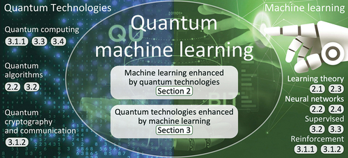
Certainly, quantum approach and relevant quantum technologies are one of the drivers of current progress in the development of information sciences and artificial intelligence, which have common goals of designing efficient computing, as well as fast and secure communication and smart IoT. The mutual overlapping of the three seminal disciplines are bearing meaningful fruits today. Within left half of the ellipsis in Figure 1 we establish some crucial topics of quantum technologies studies, which are interdisciplinary right now. In particular, quantum computing opens new horizons for classical software engineering, see e.g. [5] Especially it is necessary to mention quantum inspired algorithms and quantum inspired approaches, which utilize quantum probability and quantum measurement theory for classical computing [6].

Quantum computers as physical systems, biological neurons and human brain are capable for parallel information proceeding in natural way. However, sufficient criterion for speedup information processing is still unknown in many cases.

A qubit, which is a minimal tool in quantum information science, is established by superposition of two well-distinguished quantum states defined in Hilbert space and represents an indispensable ingredient for parallel information processing [7]. Quantum algorithms (software) which are proposed many years ago utilize qubit quantum superposition and entanglement power for achieving so-called quantum supremacy and speedup in the solution of NP-hard problems, which are unattainable with classical algorithms [8]. Quantum computers (hardware) as physical devices was first proposed by Richard Feynman, which deals with simple two-level systems as physical qubits performing quantum computation [9,10]. Despite the fact that a lot of time has passed since the successful demonstration of the first quantum gates and the simplest operations with them (see e.g. [11]), there exists a large gap between the quantum information theory, quantum algorithms, and quantum computers designed to execute them. Existing quantum computers and simulators are still very far from quantum supremacy demonstrations in solving real problems related to our daily life. This can be partly explained by the modern noisy intermediate-scale quantum (NISQ) era of the development of quantum technologies [12]. Currently, quantum computers are restricted by small number of qubits, and relatively high level of various noises, which include decoherence processes that completely (or, partially) destroy the effects of interference and entanglement. In this regard, the problem of quantum supremacy for specific tasks represents the subject of heated debates [13–15].

Surface codes and creation of logical qubits are proposed for significant reduction of computation errors [16,17]. In particular, such a code presume mapping of some graph of physical qubits onto the logical qubit. Typically, special network-like circuits are designed for quantum processor consisting of logical qubits. However, it is unclear how this mapping is unique and how such a network is optimal and universal for various computation physical platforms?

As an example, a minor embedding procedure is supposed for quantum annealing computers, which are based on superconductor quantum hardware [18]. Obviously, various physical platforms examined now for quantum computation can use different mapping procedures and relay to design of specific networks of qubits accounting specific noises and decoherence. Thus, the choosing of appropriate network architecture represents a keystone problem for current quantum computing and properly relays to demonstration of quantum supremacy.

Clearly, the solution of this problem is connected not only with the properties of quantum systems, but also with the ability of networks to parallel and robust information processing. An important example that we refer here is the human brain as a complex network comprising from biologically active networks, which exhibit fast information processing. Noteworthy, the architecture of such a computation is a non-von Neumann. In this order, the human brain is capable for pattern retrieving by means of association. A long time ago, Hopfield introduced a simple neural network model for associative memory [19]. As time evolves, neural networks have represented an indispensable tool for parallel classical computing. Artificial intelligence and machine learning paradigm, cognitive and neuromorphic computing, use neural network some specific peculiarities represent vital approach proposed to explore the full power of parallel character of computation [1,20].

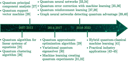
Quantum machine learning (QML) is a new paradigm of parallel computation where quantum computing meets network theory for improving computation speed-up and current, NISQ-era quantum technology facilities, by means of quantum or classical computational systems and algorithms [21–24]. In Figure 2 we represent a timeline of the appearance and development of some important algorithms [25–45] which are able to improve computational complexity, accuracy and efficiency within various types of hardware available now. In this work, we are going to discuss most of them in detail.

Figure 2. Timeline with milestones of quantum machine learning achievements.

In more general, nowadays QML disciplines occur at the border of current quantum technologies and artificial intelligence and includes all their methods and approaches to information processing, see Figure 1. The rapidly growing number of publications and reviews in this discipline indicates an increasing interest in it from the scientific community, see e.g. [46–53]. In particular, seminal problems in algorithm theory, which are capable of enhancement of quantum computing by means of the ML approach we can find in [21,46,50,53]. Some applications of ML approach to solve timely problems in material science, photonics, and physical chemistry reader can find in [47–49, 51, 52], respectively.

It is important to notice that ML approach is closely connecting with knowledge discoveries in modern fundamental physics, which are closely connected with a problem of big data and their recognition. In order, we talk about automated scientific discovery, which can significantly expand our knowledge of Nature, cf [54,55]. In particular, it is worth to mention research of the Large Hadron Collider (LHC), where data mining can contribute to new discoveries in the field of fundamental physics [56]. Another important example constitutes network research on the registration of gravitational waves and extremely weak signals in astronomy, see e.g. [57] Clearly, further discoveries in this area require improvement of the sensitivity of network detectors (which are interferometers) and obtained data mining where ML approach can significantly promote, cf [58].

Despite the fact that the previous review papers [21, 22, 46, 47, 49–53] theoretically substantiate and discuss the effectiveness of quantum approaches and quantum algorithms in ML problems, in practice there are many problems that do not allow to see quantum supremacy in experiment. Within the NISQ era of modern quantum computers and simulators, their capabilities are not yet enough to achieve quantum supremacy, cf [12]. In this regard, hybrid information processing algorithms that take into account the sharing of quantum and classical computers have come forward. Quantum-classical variational, quantum approximate optimization (QAOA) algorithms are very useful and effective in this case, see e.g. [59–62]. In this review work, we are going to discuss various approaches, which are use for QML paradigm within current NISQ-era realities. Unlike the previous work [21,22,46,47,49–53], below we will focus on methods and approaches of ML that can be effective, especially for hybrid (quantum-classical) algorithms, see Figure 2.

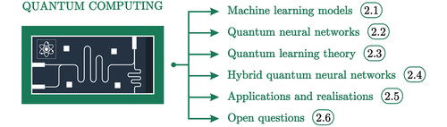
In its most general form, the current work can be divided into two large parts, which we establish as Sections 2 and 3, respectively. In particular, in Sec. 2 we consider a variety of problems where the ML approach may be enhanced by means of quantum technologies, as it is presented in Figure 1. In general, we speak here about speed-up of data processing by quantum computers and/or quantum simulators, which we can use for classical ML purposes, see Figure 3. An important part of these studies is devoted to optimal encoding, or embedding of classical data sets into the quantum device [63], and recognition of data set from quantum state readout. We establish a comprehensive analysis of quantum neural network (QNN) feature as a novel model in QML whose parameters are updated classically. We discussed how such a model may be used in timely hybrid quantum-classical variational algorithms.

Figure 3. Quantum technologies help in improving machine learning. Sections that discuss a particular topic are labeled.

On the contrary, in Sec. 3 we establish currently developing QML hot directions where classical ML approach can help to solve NISQ-era quantum computing and quantum technology tasks, cf. Figure 1. In particular, it is necessary to mention automation of quantum experiments, quantum state tomography, quantum error correction, etc., where classical ML techniques may be applied. Especially, we note here that ML algorithms which can be useful in recognition of quantum speedup problem of random (classical, or quantum) walks performed on various graphs. The solution to this problem proposed by us plays an essential role for both of current quantum computing hardware and software development.

2. Machine learning enhanced by quantum technologies

In this section, an impact that quantum technologies make in machine learning is discussed. The outline of the topics is given in Figure 3.

2.1. Machine learning models

At its roots, machine learning is a procedural algorithm that is augmented by the provision of external data to model a specific probability distribution. The data could consist of only environment variables (features), – unsupervised learning – features and their associated outcomes (labels), – supervised learning – or environment variables and a reward for specific actions, – reinforcement learning.

2.1.1. Unsupervised learning

The point of unsupervised learning is to infer attributes about a series of data points, usually to find the affinity of data points to a clustering regime. A popular method of unsupervised learning is known as the K-means clustering [64] where data points are assigned to a chosen number of clusters, and the position of the centres of these clusters could be trained. Unsupervised learning is applied to many real-world problems, from customer segmentation in different industries [65] to criminal activity detection [66].

2.1.2. Supervised learning

In contrast, supervised learning endeavours to infer patterns in the provided data. The goal of such models is to generalise this inference to previously unseen data points. In a linear regression setting, this is often done by linear interpolation [67], but for an a-priori problem where some degree of non-linearity is plausible, supervised learning can train non-linear regression models and provide better alternatives. Supervised learning is also used for logistical learning, where instead of a regression model, a categorical probability distribution is to be learned. Supervised learning has seen considerable success in many areas, from credit-rating models [68] to scientific fields [69].

2.1.3. Reinforcement learning

Finally, reinforcement learning is the optimisation of a set of actions (policy) in an environment. The environment allows actions and provides rewards if certain conditions are met. An agent is made to explore this environment by investigating the outcomes of certain actions given its current state and accordingly optimise its model variables. Reinforcement learning often attracts significant attention from the gaming industry [70] but it has also contributed to real-life scenarios, such as portfolio management [71].

2.1.4. Exponential growth of practical machine learning models

A recurring theme in all three modes of ML is the high complexity of their models. This could be caused by a high-dimensional input size like classifying a high-resolution image database [72], or a complex problem like image segmentation [73]. A commonly used – but known to be inaccurate [74,75] – measure of complexity is the parameter-count of an ML model. It is simply the number of trainable parameters of a model. Most familiarly in neural networks, the parameters are the weights and biases associated with each neural layer. For smaller problems, the parameter-count could be as small as hundreds [76,77], but cutting-edge AI models, such as DALL-E 2 [78], Gopher [79], and GPT-3 [80] are models that have tens or hundreds of billions of parameters and is increasing [81,82]. This level of high-dimensionality comes at a great financial and environmental cost. Ref [83]. assessed the carbon emission and the financial cost of fine-tuning and training several large ML models in 2019. They found that in some cases these models emitted more CO2 than the entire lifetime of an average American car, and could cost over $3 m. In addition to this great cost, there are concerns regarding the scalability, namely that the exponential-growth in computing power – known as Moore’s law [84], revisited in [85] – is growing at a slower rate than ML research [86,87].

2.1.5. Quantum-enhanced machine learning

The idea behind the field of quantum machine learning is to use the capabilities of quantum computers to provide scalable machine learning models that can provide machine learning capabilities beyond what classical models can be expected to deliver, at a healthier cost.

Quantum computers offer an exponential computational space advantage over classical computers by representing information in quantum binary digits or qubits. Where classical computers work in the Boolean space, , qubits form an exponentially growing, special unitary space, . This means that while a classical register with bits can hold an n-digit binary string, a quantum register of the same size holds all possible strings of such size, providing an exponential number of terms in comparison to its classical counterpart [7].

In addition to addressing the scalability concerns, classical machine learning models operate within the realm of classical statistical theory, which in some cases seems to diverge from human behavioural surveys. Ref [88]. Introduced the sure thing principle, which shows how unrelated uncertainties could affect a human’s decision, which a classical statistical model would deem as unrelated and remove. In Refs. [89,90] it is showed that in some cases people tend to give higher credence to two events occurring in conjunction than either happening individually, which is contrary to the classical statistical theory picture. In Ref [6,91]. It is argued that these problems could be addressed by using a quantum statistical formulation. In addition, other similar issues like the problem of negation [92] and others listed in Ref [93]. are also shown to have a resolution in the quantum theory. The distributional compositional categorical (DisCoCat) model of language [94] could be addressed as the first theoretically successful attempt at harnessing this advantage of quantum machine learning.

2.2. Quantum neural networks

For a given data provision method, e.g. supervised learning, a host of different machine learning architectures could be considered. A machine learning architecture has a set of trainable parameters that can be realised based on an initial probability distribution. Any specific realisation of the parameters of a machine learning architecture is a model. The quest of machine learning is to train these parameters and achieve a nearer probability distribution to that of the problem in question. The fully trained version of each architecture yields a different model with different performance, and generally, the architectures that can spot and infer existent patterns in the data are said to be of superior performance. It is also important to avoid models that find non-existent patterns, models that are said to over-fit their pattern-recognition to the provided data, and when evaluated on previously unseen data fail to perform as well. A model that can spot existent patterns without overfitting to the provided data is said to have a high generalisation ability. This metric establishes a platform for model selection¹ [95].

For any given problem, there are a variety of architecture classes to choose from. Some of the most commonly used architectures are multi-layered perceptrons (neural networks), convolutional networks for image processing, and graph neural networks for graphically structured data. QML contributes to this list by introducing quantum models such as QNN [96].

Quantum neural networks are models in QML whose parameters are updated classically. The training pipeline includes providing data to the quantum model, calculating an objective (loss) value, and then adapting the QNN parameters in such a way as to reduce this objective function. A specific approach to providing the data to the quantum model is known as the data encoding strategy, and it can have a drastic effect on the functional representation of the model. Sec 2.2.1 covers the various approaches to data encoding, and Sec 2.2.4 offers a review of the theoretical advances in exploring the analytical form of this representation. In QNNs, the objective function is (or includes) the expectation value of a parametrised quantum circuit (PQC) [97]. PQCs are quantum circuits that make use of continuous-variable group rotations. Fine-tuning the architecture of the PQC can have a direct effect on the performance of the resultant QNN model. Sec 2.2.2 reviews the various PQC parametrisations suggested in the literature.

The consequences of the choice of the loss function are outlined in Sec 2.3.1. After making this choice, one could evaluate the PQC, and pass the result to the loss function to obtain a loss value. To minimise the loss value, it is important to tune the trainable parameters in such a way to maximally minimise this value. This is achieved – in both the classical and quantum ML – by calculating the gradient of the loss function with respect to the model parameters.² The gradient vector of a function point to the direction of maximal increase in that function, and to maximally reduce the loss function one could find the gradient and step in the opposite direction. Sec 2.2.3 reviews the literature concerning QNN gradient computation.

2.2.1. Data encoding strategies

There are three overarching data encoding strategies [98]:

• State embedding: the features are mapped to the computational bases. This is often used for categorical data, and as the number of bases grows, the number of data points needs to follow the same trend, otherwise, the encoding will be sparse [96].

• Amplitude embedding: when the features of the dataset are mapped to the amplitudes of the qubit states. This embedding could be repeated to increase the complexity of the encoding. For qubits, this method allows us to encode up to features onto the quantum system.

• Observable embedding: the features are encoded in a Hamiltonian with respect to which the quantum system is measured. This encoding is typically used in quantum native problems - see Sec 2.5.2 - namely variational quantum eigensolvers (VQE) [30] and quantum differential equation solvers [99,100].

It is important to recognise that state embedding is the only discrete-variable encoding with a strong resemblance to classical ML, whereas the other two are continuous-variable methods and can be considered analogue machine learning.³

Amplitude embedding could be sub-divided into sub-categories: angle embedding, state amplitude embedding, squeezing embedding and displacement embedding [101,102]. Ref [98]. provides an expressivity comparison between these encoding methods. Effective encoding strategies were analysed in [99,103–105].

2.2.2. Parametrised architecture

The specific parametrisation of the network could dramatically change the output of a circuit. In classical neural networks, adding parameters to a network improves the model expressivity, whereas, in a quantum circuit, parameters could become redundant in over-parametrised circuits [106]. Additionally, the architecture must be trainable, whereas it was shown that this cannot be assumed in an a-priori setting [107] – see Sec 2.2.5. Many architectures have been suggested in the literature, and many templates are readily available to choose from on QML packages [108–110].

Ref [111]. introduced a family of hardware-efficient architectures and used them as variational eigensolvers – see Sec 2.5.2. These architectures repeated variational gates and used CNOT gates to create highly entangled systems. Based on the discrete model in Ref [112]. and made continuous in Ref [113]. A model was devised using RZZ quantum gates that was shown to be computationally expensive to classically simulate [101,114,115], named the instantaneous polynomial-time quantum ansatz (IQP).

Another approach to creating quantum circuits is to take inspiration from tensor networks [116]. Famous architectures in this class are the tensor-tree network (TTN), matrix product state (MPS), and the quantum convolutional neural networks (QCNN) [34,117–119].

2.2.3. Gradient calculation

Despite its excessive memory usage [120], the most prominent gradient calculation method in classical ML is the back-propagation algorithm [121]. This method computes the gradient of every function that trainable parameters are passed through alongside its output and employs the chain rule to create an automatically differentiable ML routine. The back-propagation method can (and has been [122]) implemented for QML, but as it requires access to the quantum state-vector, it can only be used on a simulator and not a real quantum processing unit (QPU). As quantum advantage can only occur in the latter setting, it is important to seek alternatives that can operate on QPUs.

The first proposed algorithm is known as the finite-difference differentiation method [123]. As its name suggests, it calculates the gradient by using the first principles of taking derivatives, i.e. adding a finite difference to the trainable parameters one at a time, and observing the change that this action makes. This method is prone to error in the NISQ era.

As an alternative, a discovery was made in [124] known as the parameter-shift rule that suggested an exact, analytic derivative could be calculated by evaluating the circuit twice for each trainable parameter. The suggestion was that the derivative of a circuit with respect to a trainable parameter is half of the evaluation of the circuit with shifted by subtracted from the circuit when it is shifted by . This suggestion initially worked only on trainable parameters applied to Pauli rotations, but later works [125–132] expanded to its current form, applicable to any parametrisation. The parameter-shift rule is the state-of-the-art gradient computation method and is compatible with QPUs, but one of its major problems is its scalability. As mentioned, the number of circuit evaluations for this method increases linearly with the number of trainable parameters, and this poses a challenge to how complex the quantum models can get. A notable effort to mitigate this effect was by parallelising the gradient computation, which is now natively provided when using PennyLane on AWS Braket [133].

As a transitional gradient computation method for QNNs, Ref [134]. introduced the adjoint algorithm. Similar to the back-propagation method, the adjoint can only be run on a simulator and calculates the entire gradient vector using a single evaluation of the circuit. However, its memory usage is superior to the former. It works by holding a copy of the quantum state and its adjoint in the memory, and in turn applying the gates in reverse order, calculating the gradients wherever possible. This means that two overall evaluations of the circuit are made, first to evaluate the output, and second to compute the gradient.

Alternative suggestions have also been made to optimise QML models following the geometry of their group space. Ref [135]. suggested a Riemannian gradient flow over the Hilbert space, which through hardware implementation showed its favourable optimisation performance.

2.2.4. Quantum neural networks as universal Fourier estimators

Ref. [105] explored the effects of data encoding on the expressivity of the model. It is proved that the data re-uploading technique suggested by Ref [136]. created a truncated Fourier series limited by the number of repetitions of the encoding gates. Ref [137]. also showed that QNNs can be universal Fourier estimators – an analogue to the universality theorem in classical multi-layered perceptrons [138]. Another point proven by Refs. [105,136] was that by repeating the encoding strategy (in amplitude embedding and more specifically the angle embedding) more Fourier bases are added to the final functional representation of the circuit. This was true if the repetitions were added in parallel qubits or series. This sparked a question about the accessibility of these Fourier bases, i.e. whether their coefficients can independently be altered, which remains an open question at the time of this publication.

2.2.5. Barren plateaus and trainability issues

QNNs could suffer from the problem of vanishing gradients. This is when during training, the gradient of the model tends to zero in all directions. This could severely affect the efficiency of the training or even bring it to a halt. This is known as the barren plateau (BP) problem.

BPs are not usually at the centre of attention in classical ML, but their dominance in quantum architectures makes them one of the most important factors in choosing a circuit. Ref [107]. showed that the expectation value of the derivative of a well-parametrised⁴ quantum circuit is equal to zero, and that its variance decays exponentially with the number of qubits. Ref [139]. confirmed that barren plateaus also exist in gradient-free optimisation methods. In addition, Ref [140]. showed that in the NISQ era, using deep circuits flattens the overall loss landscape resulting in noise-induced BPs. These are mathematically different kinds of Barren plateaus that flatten the landscape as a whole. Illustrations in Figure 4 summarise these phenomena.

Figure 4. Visualisation of the barren plateau phenomenon in (a) noise-free and (b) noise-induced settings.

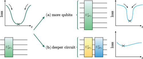
These two findings painted a sobering picture for the future of QNNs, namely that they need to be shallow and low on qubit-count to be trainable, which contradicts the vision of high-dimensional, million-qubit QML models.

Many remedies have been proposed: Ref [141]. suggested that instead of training all parameters at once, the training could be done layer-wise and Ref [142]. showed that if the depth of the variational layers of the QNN is of the order O(), being the number of qubits, and that only local measurements are made, the QNN remains trainable. This was tested on circuits with up to 100 qubits and no BPs were detected. Other remedies included introducing correlations in the trainable parameters [143,144] and specific initialisations of the parameters [145] of the circuit by applying adjoint operators of certain variational gates.

More analysis was done on specific architectures: Ref [146]. showed that under well-defined weak conditions, the TTN architecture was free from the BP problem; and Ref [147]. showed that the quantum convolutional neural network architecture introduced in Ref [34]. was also free from BPs. Ref [148]. developed a platform based on ZX calculus⁵ to analyse whether a given QNN is subject to suffering from BPs. In addition to confirming the results from the two earlier contributions, it is also proved that the matrix product state [149] and hardware efficient, strongly-entangling QNNs suffered from BPs. Furthermore, Ref [150]. related the barren plateau phenomenon to the degree of entanglement present in the system.

2.3. Quantum learning theory

2.3.1. Supervised QML methods are kernel methods

In Refs. [98,151] the similarities between the QNNs and kernel models were brought to focus. First introduced in Ref [152]., kernel methods are well-established ML techniques with many applications. In conjunction with support vector machines (SVM), the way they work is by mapping the features of a dataset into a high-dimensional space through a function and then using a kernel function, , as a distance measure between any two data points in this high-dimensional space. This is exactly the behaviour observed in QNNs: the features are first embedded into a high-dimensional quantum state-vector, and by overlapping one encoded state with another we can find the level of similarity between two points in this space. In this high-dimensional space, one hopes to find better insight into the data – usually expressed as a decision boundary in the form of a hyperplane in classification tasks. Ref [153]. used this link and developed a framework for searching for possible quantum advantages over classical models. It is also shown that large models could scatter the data so far apart that a distance measure becomes too large for optimisation purposes, and proposed that an intermediate step be added to map the high-dimensional space into a lower-dimensional hyperplane to improve its training performance.

2.3.2. Bayesian inference

Bayesian inference is an alternative approach to the statistical learning theory where Bayes’ theorem [154] is used to adapt an initial assumption about the problem (prior distribution) based on newly-found data (evidence) to get a posterior distribution. Bayesian learning is when this logic is applied to ML. This is done by applying a distribution to every parameter in the network and updating the distributions when training. Calculating the posterior distribution is generally computationally expensive, but it is possible to approximate its using a trick known as variational inference [155,156] successfully demonstrated an approximate back-propagation algorithm on a Bayesian neural network (BNN), referred to as Bayes-by-backprop.

The first implementations of Bayesian QNNs were in Refs. [157–159] which attempted to make quantum circuits into an exact Bayesian inference machine. Ref [160]. introduced two efficient, but approximate methods – one from kernel theory and another using a classical adversary – to use QNNs to perform variational inference. The work consists of a quantum circuit that can be modelled to produce the probability distribution of a phenomenon by exploiting the probabilistic nature of quantum mechanics – known as a Born machine [161,162] or quantum generative models [149,163–168]. This could also be used later to quantify the prediction error for a single data point, as it has been done classically in Ref [169].

2.3.3. Model complexity and generalisation error bounds

Intuitively, complex phenomena require complex modelling, but quantifying the complexity of a given model is non-trivial. There are multiple ways of defining the model complexity: Vapnik-Chervonenkis (VC) dimension [170], Rademacher complexity [171], and effective dimension [172].⁶ The complexity measures are also connected to the generalisation error because when the model becomes too complex for the problem, the generalisation is expected to worsen.

Much work has been done to quantify the complexity and the generalisation error of quantum neural networks: Ref [173]. explored a generalisation error bound through the Rademacher complexity that explicitly accounted for the encoding strategy; and Ref [174]. used the effective dimension – a measure dependent on the sample size – to bound the generalisation error of QNNs as well as prove their higher expressivity given the same number of trainable parameters. Other attempts were also made to quantify the complexity (also referred to as the expressivity) of QNNs in Refs. [175–179].⁷ Notably, Ref [180]. theoretically proved that the generalisation error of a QNN grew as where was the number of parametrised quantum gates in the QNN, and was the number of data samples in the dataset. The latter work implies that QML models are better at generalising from fewer data points.

2.4. Hybrid quantum neural networks

Just as there are classical and quantum models, one could also combine the two to create hybrid models – see Figure 5. It is conceivable that in the NISQ era, one could use the understanding of QML described in Sec. 2.3 to find a regime where quantum models cover some bases that classical models do not. Ref [41]. developed a platform for hybrid quantum high-performance computing (HQC) cloud and it was deployed on the QMware hardware [181,182]. It is shown that for high-dimensional data, a combination of classical and quantum networks in conjunction could offer two advantages: computational speed and the quality of the solution. The data points were, first, fed to a shallow⁸ quantum circuit composed of four qubits, two of which were measured, and their corresponding values were passed onto a neural network. Two classical datasets were chosen to explore the effectiveness of a hybrid solution and to compare it when the quantum part is removed, leaving only a classical network: the sci-kit circles’ dataset [183] and the Boston housing dataset [184]. The former is a synthetic geometrical dataset that consists of two concentric circles in a 2-dimensional square of side , and the latter is about the distribution of the property value given its population status and the number of rooms. In both cases, it was shown that the hybrid network generalises better than the classical one and this difference is most visible at the extremes of problems with very small training sample sizes. However, this difference became smaller as the number of samples grew.

Figure 5. An example of a hybrid quantum-classical ML model. In this case, the inputs are passed into a fully connected classical multi-layered perceptron, and its outputs are fed into the embedding of a quantum circuit. Depending on the setting, some measurements of this quantum circuit are taken and then passed into another fully connected layer, the output of which can be compared with the label.

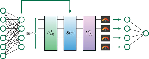
In continuation, Ref [44]. suggested a hyperparameter optimisation scheme aimed at architecture selection of hybrid networks. This work also implemented a hybrid network for training, but in two new ways: 1) using a real-world, image recognition dataset [185], and 2) the quantum part of the hybrid network was inserted in the middle of the classical implementation. Additionally, the architecture of the quantum part was a subject of hyper-parameter optimisation, namely the number of qubits used, and the number of repetition layers included are optimised. Training this network showed that the hybrid network was able to achieve better quality solutions, albeit by a small margin. It is notable that because of this architecture optimisation, a highly improved quantum circuit was achieved. The performance of this circuit was theoretically measured by applying analysis methods such as ZX reducibility [186], Fourier analysis [105], Fisher information [106,187,188], and the effective dimension [172,174].

2.5. Applications and realisations

QML automatically inherits all classical ML problems and implementations, as it is simply a different model to apply to data science challenges. In addition to this inheritance, QML research has also provided novel, quantum-native solutions. In both cases, QML has so far been unable to provide a definite, practical advantage over classical alternatives, and all the suggested advantages are purely theoretical.

2.5.1. Solving classical problems

QML is employed in many classical applications. Some notable contributions are in sciences [189–195], in finance [42,196–198], pharmaceutical [43,45], and automotive industries [44]. In many cases, these models replaced a previously known classical setting [199–202]. Quantum generative adversarial networks were suggested in Ref [203]. and followed by Refs. [204–211]. Similarly, quantum recurrent neural networks were investigated in [212,213], and two approaches to image recognition were proposed in Refs. [34,214]. Ref [215]. looked at a classical-style approach to quantum natural language processing. The applications of QML in reinforcement learning were also explored in Refs. [38,216–218].⁹ Finally, a celebrated application is the quantum auto-encoder, where data is compressed and then re-constructed from less information, a notable suggestion was made in Ref [219].

2.5.2. Quantum-native problems

Native problems are novel, quantum-inspired ML problems that are specifically designed to be solved by a QML algorithm.

Perhaps, the most known QML algorithm is the variational quantum eigensolver (VQE). The problem formulation is that the input data is a Hamiltonian, and we are required to find its ground state and ground-state energy. The VQE solution consists of preparing a PQC of trainable parameters and taking the expectation value of the Hamiltonian. This yields the energy expectation of the prepared state, and the idea is that by minimising this expectation value, we can achieve the ground-state energy, at which point the prepared state will represent the ground state of the problem. This was first implemented to find the ground-state energy of [30] and was then substantially extended in Ref [59]. VQE remains one of the most promising areas of QML.

Ref [25]. showed that PQCs can be used to solve a linear system of equations (LSE). They proposed a commonly known as the Harrow, Hassidim, and Lloyd (HHL). Refs. [220–227] improved this algorithm and Ref [228]. extended it to also include non-linear differential equations. Ref [100]. showed that it is possible to use a quantum feature map to solve non-linear differential equations on QNNs. This is also an exciting and promising area of QML.

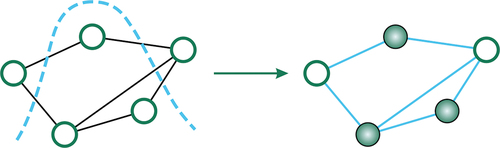
An important QML formulation is known as the quadratic unconstrained binary optimisation (QUBO) [229,230]. This is generally a classical problem, but using the Ising model – see [231] – this can be solved on a quantum computer [232,233]. A common demonstration of the latter is the max cut problem [234] – see Figure 6. There are solutions for the QUBO problem on both gate-based quantum computers and quantum annealers [235–237], and this general concept has seen use in many sectors [238].

Figure 6. The max cut problem. The abstract manifestation of this problem is a general graph, and we are interested in finding a partition of its vertices such that the number of edges connecting the resultant graph to the complementary graph is maximal.

Lastly, another quantum-native formulation is in natural language processing. Ref [94]. developed a platform for turning grammatical sentences into quantum categories using J. Lambek’s work [239]. Refs. [240–242] tested this algorithm on quantum hardware, and later a full QNLP package was developed [243]. The initial value proposition of QNLP in this way is that this algorithm is natively grammar-aware, but given that large classical language models are shown to infer grammar [80], the real advantage of this approach could lie in other avenues, such as a potential Grover-style [244] speed-up in text classification.

2.6. Open questions

2.6.1. Quantum advantage

Despite the theoretical findings in Sec 2.3.3, there is limited demonstrable success in using QML in real-life problems, and this is not purely due to hardware shortcomings. Ref [245]. showed that there exists a class of datasets that could showcase quantum advantage, and Ref [153]. found a mathematical formulation for where we can expect to find such an advantage. In Refs. [246–248] attempts were also made to devise a set of rules for potential quantum advantage. However, Ref [249]. argued that a shift of perspective from quantum advantage to alternative research questions could unlock a better understanding of QML. The suggested research questions were: finding an efficient building block for QML, finding bridges between statistical learning theory and quantum computing, and making QML software ready for scalable ML.¹⁰

2.6.2. Optimal parametrisation

In Sec 2.2.2, we encountered various QNN parametrisations with specific properties. An open question is how to optimally parametrise a circuit to avoid barren plateaus, be as expressive as possible, and be free of redundancy. A potential characteristic of such a parametrisation is a high level of Fourier accessibility as mentioned in Sec 2.2.4, potentially requiring a quantifiable measure of this accessibility.

2.6.3. Theory for hybrid models

Despite the successes outlined in Sec 2.4, the theoretical grounding for such models is limited. We saw that hybrid networks performed well if the quantum section was introduced at the beginning of the model architecture [41] or in the middle [44]. From an information-theoretic perspective, this needs to be investigated in more detail to shed light on the effect of hybridisation. Such investigation could identify if there exist areas where the application of a quantum part could complement a classical circuit by either introducing an information bottleneck to prevent over-fitting or by creating high-dimensional models.

2.6.4. An efficient optimisation method

The current gradient calculation methods are either only available on simulators or require a linearly-growing number of circuit evaluations- see Sec. 2.2.3. Neither of these can accommodate a billion-parameter, million-qubit setting. This poses a barrier to the future of QML, and thus an efficient optimisation method is needed for the long term.

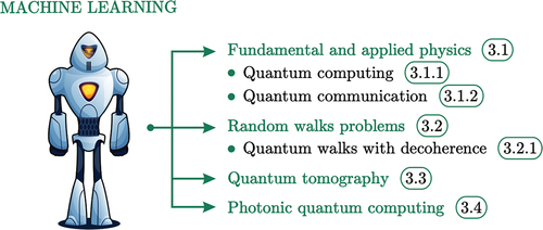
3. Quantum technologies enhanced by machine learning

In this section, an impact that machine learning makes in quantum technologies is discussed. The outline of the topics is given in Figure 7. Today machine learning is used to realize algorithms and protocols in quantum devices, by autonomously learning how to control [35,250–253], error-correct [36,254–256], and measure quantum devices [257]. Given the experimental data, ML can reconstruct quantum states of physical systems [258–261], learn compact representations of these states [262,263], and validate the experiment [264]. In this section, we discuss the impact of machine learning on fundamental and applied physics, and give specific examples from quantum computing and quantum communication.

Figure 7. Machine learning helps in solving problems in fundamental and applied quantum physics. Sections that discuss a particular problem are labeled.

3.1. Machine learning in fundamental and applied quantum physics

Since its full development in the mid-1920s, a century later quantum mechanics is still considered as the most powerful theory, modeling a wide range of physical phenomena from subatomic to cosmological scales with the most precise accuracy. Even though the measurement problem and quantum gravity had led many physicists to conclude that quantum mechanics cannot be a complete theory, the spooky action of entanglement in the Einstein-Podolsky-Rosen pair [265], has provided the resources for quantum information processing tasks. With machine learning, one may be able to model different physical systems (e.g. quantum, statistical, and gravitational) using artificial neural networks, which might lead to the development of a new framework for fundamental physics.

Even without a precise description of a physical apparatus and solely based on measurement data, one can prove the quantumness of some observed correlations by the device-independent test of Bell nonlocality [266]. In particular, by using generative algorithms to blend automatically many multilayer perceptrons (MLPs), a machine learning approach may allow the detection and quantification of nonlocality as well as its quantum (or postquantum) nature [267–269].

3.1.1. Machine learning in quantum computing

Machine learning has also become an essential element in applied quantum information science and quantum technologies. ML, which was inspired by the success of automated designs [31], was demonstrated to be capable of designing new quantum experiments [32].

Quantum experiments represent an essential step towards creating a quantum computer. More specifically, for example, three-particle photonic quantum states represent a building block for a photonic quantum computing architecture. In Ref [32]. ML algorithm used is a reinforcement learning algorithm based on the projective simulation model [270–275]. An agent, the reinforcement learning algorithm, puts optical elements on a (simulated) optical table. Each action adds an optical element to an existing setup. In case the resulting setup achieves the goal, e.g. creates a desired multiphoton entangled state, the agent receives a reward. The described learning scheme is depicted in Figure 8(a).

Figure 8. A reinforcement learning algorithm that designs a quantum experiment. An experiment on an optical table is shown as an example. (a) The learning scheme depicts how an agent, the reinforcement learning algorithm, learns to design quantum experiments. (b) Representation of the reinforcement learning algorithm, projective simulation, as a two-layered network of clips.

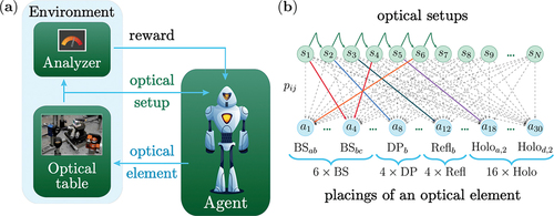
The initial photonic setup is an output of a double spontaneous parametric down-conversion (SPDC) process in two nonlinear crystals. Neglecting these higher-order terms in the down-conversion, the initial state can be written as a tensor product of two orbital angular momentum entangled photons,

(1)

where the indices and specify four arms in the optical setup. The actions available to the agent consist of beam splitters (BS), mirrors (Refl), shift-parametrized holograms (Holo), and Dove prisms (DP). The final photonic state is obtained by measuring the arm , and post-selecting the state in the other arms based on the measurement outcome in .

The reinforcement learning algorithm that achieves the experimental designs is shown in Figure 8(b). It is the projective simulation agent is represented by a two-layered network of clips. The first layer corresponds to the current state of the optical setup, whereas the second layer is the layer of actions. The connectives between layers define the memory of the agent, which changes during the learning process. The connectivities correspond to the probabilities of reaching a certain action in a given state of a quantum optical setup. During the learning process, the agent automatically adjusts the connectivities, and thereby prioritize some actions other than the other. As shown in Ref [32]. this leads to a variety of entangled states of improved efficiency of their realization.

3.1.2. Machine learning in quantum communication

In addition to designing new experiments, ML helps in designing new quantum algorithms [276] and protocols [277]. Designing new algorithms and protocols has similarities to experiment design. In particular, similar to experiment design, every protocol can be broken down into individual actions. In the case of the quantum communication protocol, these actions are, e.g: apply -gate to the second qubit, apply -gate to the first qubit, send the third qubit to the location , and measure the first qubit in the -basis. Because of the combinatorial nature of the design problem, the number of possible protocols grows exponentially with the number of available actions. For that reason, a bruteforce search of a solution is impossible for an estimated number of possible states of a quantum communication environment [277].

A reinforcement learning approach to quantum protocol design, first proposed in Ref [277]., is shown to be applicable to a variety of quantum communication tasks: quantum teleportation, entanglement purification, and a quantum repeater. The scheme of the learning setting is shown in Figure 9. The agent perceives the quantum environment state, and chooses an action based on the projective simulation deliberation process. The projective simulation network used in this work is similar to the one in Figure 8(b), with addition of hierarchical skill acquisition. This skill is of particular importance in the long-distance quantum communication setting, which has to include multiple repeater schemes.

Figure 9. A reinforcement learning algorithm that designs a long-distance quantum communication protocol. The algorithm is based on projective simulation with episodic and compositional memory (ECM). Given the state of the quantum communication environment, the algorithm chooses how to modify this state by acting on the environment. The goals of the PS agent are: (a) teleportation protocol (b) entanglement purification protocol (c) quantum repeater protocol (d) quantum repeater protocol for long-distance quantum communication.

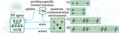
With the help of projective simulation, it was demonstrated that reinforcement learning can play a helpful assisting role in designing quantum communication protocols. It is shown that the use of ML in the protocol design is not limited to rediscovering existing protocols. The agent finds new protocols that are better than existing protocols in case optimal situations lack certain symmetries assumed by the known basic protocols.¹¹

3.2. Machine learning in random walks problems

Random walks paradigm plays an important role in many scientific fields related to the transfer of charge, energy, or information transport [278–282]. Random (classical) walks on graphs represent an indispensable tool for many subroutines in computational algorithms [283–285]. Quantum walks (QW) represent a generalization of classical walks to the quantum domain and use quantum particles instead of classical one [286,287]. The resulting quantum interference pattern, which governs the QW physics fundamentally differs from the classical one [288]. For quantum information science, it is crucially important that a quantum particle exhibits quantum parallelism, which appears as a result of various path interference and entanglement. It was shown that quantum particle propagates quadratically faster than classical one on certain graphs, which are line [289], cycle [290,291], hypercube [292,293] and glued trees graphs [294], respectively. It is expected that algorithms based on QW should demonstrate quadratic speedup that is . Such parallelism may be useful for quantum information processing and quantum algorithm purposes [294–296]. It is especially important to note that QWs are explored in quantum search algorithms, which represent important tools for speed up of QML algorithms [21,297–299].

Noteworthy, QW speed up demonstration with arbitrary graphs represents an open problem [300]. The standard approach would be to simulate quantum and classical dynamics on a given graph, which provides an answer in which case a particle would arrive at a target vertex faster. However, this approach may be difficult (and costly) to use in computations for the graphs possessing a large number of vertices; the propagation time scales polynomially in the size of the graph. Second, we are usually interested in a set of graphs for which the obtained results of the simulations cannot reveal some general features of quantum advantage.

In a number of works, we attacked this problem by means of ML approach [39,40,301]. We explore a supervised learning approach to predict a quantum speed up just by looking at a graph. In particular, we designed a classical-quantum convolutional neural network (CQCNN) that learns from graph samples to recognize the quantum speedup of random walks.

The basic concept of CQCNN that we use in Ref [39,40,301]. is shown in Figure 10 and Figure 11, respectively. In particular, we examined in Ref [39,40,301–303]. continuous-time random walks and suppose that the classical random walk representing stochastic (Markovian) process defined on a connected graph. It starts at the time from the initial node and hits the target vertex. Unlike the classical case, a quantum particle due to interference phenomenon will be ‘smeared’ across all vertices of the graphs. Thus, in the quantum case, we propose an additional (sink) vertex that is connected to the target vertex and provides localization of the quantum particle due to energy relaxation from to vertices, which happen with the rate . In other words, the quantum particle may be permanently monitored at the sink vertex. Mathematically, a graph is characterized by its weighted adjacency matrix that is relevant to Hamiltonian . Notice, for chiral QW time asymmetry may be obtained by using complex-valued adjacency matrix elements [301]. We characterize quantum transport by means of Gorini–Kossakowski–Sudarshan–Lindblad equation that looks like (cf [304].):

Figure 10. A schematic representation of considered in Refs. [39,40] random walks on (a) connected random graph, (b) cycle graph. The labels (), and () specify initial and target vertices, respectively; is a sink vertex which is require to localize and detect quantum particle. The is coupling parameter between target and sink vertices, respectively.

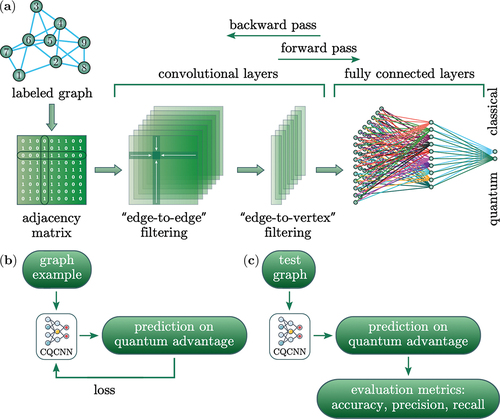
Figure 11. Schematic representation of CQCNN approach which is used for predicting the quantum speed up on the graphs represented in Figure 10. (a) – scheme of the CQCNN architecture. The neural network takes a labeled graph in form of an adjacency matrix as an input. The then processed by convolutional layers with filters of graph-specific ‘edge-to-edge’ and ‘edge-to-vertex’, respectively. These filters act as functions of a weighted total number of neighboring vertices of each vertex. The convolutional layers are connected with fully connected layers which classify the input graph. Data and error propagation are shown with arrows. (b) and (c) demonstrates processes of CQCNN training and testing, respectively.

(2)

where is time-dependent density operator, and operators characterize transitions from vertices to and from (target) to (sink), respectively; is the coupling parameter between target and sink vertices. The parameter lies condition and determines the decoherence; the value is relevant to purely quantum transport, while determines completely classical random walks.

The solution of Eq. (2)(2) specifies quantum probability ( is the total number of vertices), which is relevant to QW on a chosen graph. The classical random walk may be established by the probability distribution

(3)

where is a vector of probabilities of detecting a classical particle in vertices of the graph; is the identity matrix of size . The transition matrix is a matrix of probabilities for a particle to jump from to . In this case, the sink vertex is not needed, and we can assume . We are interested in the probability of finding a particle in the target (or, in the sink) vertex, which is described by solutions of Eq. (2)(2) and (3(3) ).

Then, one is possible to compare and against that determines threshold value of probability for a given graph. If this probability is larger than , we can conclude that the particle occurs at the target. The time at which one of the inequalities , fulfilled, is called the hitting time for quantum or classical particle, respectively. Hence, by comparing the solutions to Eq. (2)(2) and (3(3) ), we can define the particle transfer efficiency: it is if the quantum particle reached the target first, and otherwise.

In Figure 11 we schematically summarize the proposed CNN approach for detection of QW speedup. In order, the architecture of CQCNN is shown in Figure 11(a). It consists of a two-dimensional input layer that takes one graph represented by an adjacency matrix . This layer is connected to several convolutional layers, the number of which depends on the number of vertices of the input graph. The number of layers is the same for all graph sizes. CQCNN has a layout with convolutional and fully connected layers, and two output neurons that specify two possible output classes. Convolutional layers are used to extract features from graphs, and decrease the dimensionality of the input.

Empirically, we find out that relevant features are in the rows and columns of adjacency matrices. The first convolutional layer comprises six filters (or, feature detectors) which define three different ways of processing the input graph. These three ways are marked by green, red, and blue colors in Figure 11(a), respectively. The constructed filters are form ‘crosses’ which are shown in Figure 11(a) and capture a weighted sum of column and row elements. These filters act as functions of a weighted total number of neighboring vertices of each vertex. Thus, the cross ‘edge-to-edge’ and ‘edge-to-vertex’ filters crucially important in designed CQCNN; they are capable for prediction of the quantum advantage by QW.

Figure 11(b) shows schematically the training procedure by using some graphs samples, which are established by adjacency matrices as an input. CQCNN made prediction at the output determining classical or quantum classes depending on the values of the two output neurons. The predicted class is determined by means of the index of a neuron with the largest output value . Having a correct label, the loss value is computed.

The filters that we constructed in CQCNN play an essential role in the success of learning. CQCNN learns by stochastic gradient descent algorithm that takes the cross-entropy loss function. The loss on a test example is defined relative to the correct class (classical or quantum, or ) of this example:

(4)

where we defined the values of the output neurons as and ; is the total fraction of examples from this class in the dataset. As we have shown in Ref [39]. CQCNN constructed a function that generalizes over seen graphs to unseen graphs, as the classification accuracy (which may be defined as the fraction of correct predictions) goes up.

CQCNN testing procedure is not principally different from the training process in how it is seen in Figure 11(c), cf. Figure 11(b). The CQCNN does not receive any feedback on its prediction in this case and the network is not modified.

We apply the described ML approach to different sets of graphs. In particular, to understand how our approach works in a systematic way, we first analyze the CQCNN on line graphs with up to vertices. CQCNN was trained over epochs with a single batch of examples per epoch.

Then, we simulated CQCNN’s learning process for random graphs, each sampled uniformly from the set of all possible graphs with vertices and edges. The learning performance results in the absence of decoherence () are shown in Figure 12 for ; the is chosen uniformly from to . Our simulations shows that the loss after training is vanishing; it is below for all these random graphs. 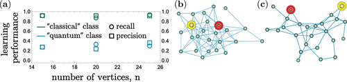In Figure 12(a) we see that both recall and precision are about for the ‘classical’ part of the set, and is in the range of for the ‘quantum’ one. n¹² Thus, one can see that CQCNN helps to classify random graphs correctly much better than a random guess without performing any QW dynamics simulations. In Figure 12(b)-(c) we represent samples of correctly classified graphs.

Figure 12. (a) CQCNN learning performance. Dataset consists of random graphs with and vertices, examples for each , and the corresponding classical and quantum labels. CQCNN was simulated during epochs, mini batches each with the batch size of examples. The neural network was tested on random graphs for each . (b), (c) establish random graph examples taken from the test set which were correctly classified by CQCNN (initial and target vertices are marked in yellow and red, respectively). The classical particle is faster on (b), whereas the quantum one is faster on graph (c).

3.2.1. Quantum walks with decoherence

In the presence of decoherence, i.e. for physical picture is getting richer. In Figure 13 we demonstrate results of QW dynamics simulation on cycle graph consisting of -vertices; the efficiency of transport is measured between opposite vertices of the graph as it is shown in Figure 10(b). Simulations are performed for randomly sampled values of the decoherence parameter and used to train CQCNN. After the training procedure, we suggest CQCNN to predict if the QW can lead to an advantage for a new given parameter . In Figure 13, we represent the results of the transfer efficiency predictions as a violet line. From Figure 13 it is clearly seen that at the value of decoherence parameter abrupt crossover from quantum () to classical () regime transport occurs. Thus, one possible to expect QW advantage in transport in domain of . Physically, such a crossover may be relevant to quantum tunneling features in the presence of dissipation, cf [305,306]. Notice that the parameter is temperature-dependent in general, cf [307]. In this case, we can recognize the established crossover as a (second-order) phase transition from the quantum to classical (thermal activation) regime that happens for a graph at some finite temperature.

Figure 13. Prediction of transfer efficiency (violet curve) for a -cycle graph versus decoherence parameter . The activation values of output neurons are shown in blue and green. The results obtained by averaging of CQCNN networks. Standard deviations are marked by shaded regions.

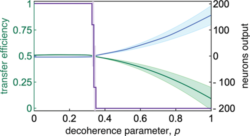
Figure 13 demonstrates predictions of CQCNN which are based on the learned values of the output neurons; they are shown in Figure 13 as a classical (blue) and quantum (green) classes, respectively. CQCNN made decision about the class by using the maximum value of the output neuron activation. From Figure 13 it is clearly seen that the ‘vote’ for the quantum class grows up to the maximum value , which corresponds to the highest confidence for the quantum class. Simultaneously, the confidence in the classical class grows with increasing of decoherence parameter . Separation between the classes becomes more evident after the crossover point of .

Thus, the obtained results play a significant role in the creation of soft- and hardware systems, which are based on the graph approach at their basis. CQCNN that we proposed here allows us to find out which graphs, and under which conditions on decoherence, can provide a quantum advantage. This is especially relevant to NISQ era quantum devises development.

3.3. Machine learning in quantum tomography

With the capability to find the best fit to arbitrarily complicated data patterns with a limited number of parameters available, machine learning has provided a powerful approach for quantum tomography. Here, quantum tomography or quantum state tomography (QST) refers to the reconstruction about a quantum state with its comprehensive information by using measurements on an ensemble of identical quantum states [308–314]. However, the exponential growth in bases for a Hilbert space of -qubit states implies that exact tomography techniques require exponential measurements and/or calculations. In order to leverage the full power of quantum states and related quantum processes, a well characterization and validation of large quantum systems is demanded and remains an important challenge [315].

Traditionally, by estimating the closest probability distribution to the data for any arbitrary quantum states, the maximum likelihood estimation (MLE) method is used in quantum tomography [316,317]. However, the MLE method requires exponential-in- amount of data as well as an exponential-in- time for processing. Albeit dealing with Gaussian quantum states, unavoidable coupling from the noisy environment makes a precise characterization on the quantum features in a large Hilbert space almost unattackable. Moreover, MLE also suffers from the overfitting problem when the number of bases grows. To make QST more accessible, several alternative algorithms are proposed by assuming some physical restrictions imposed upon the state in question, such as the adaptive quantum tomography [318], permutationally invariant tomography [319], quantum compressed sensing [320–323], tensor networks [324,325], generative models [326], feed-forward neural networks [327], and variational autoencoders [328].

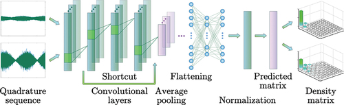
To reduce the overfitting problem in MLE, the restricted Boltzmann machine (RBM) [329–332] has provided a powerful solution in QST. With the help of two layers of stochastic binary units, a visible layer and a hidden layer, the RBM acts as a universal function approximator. For qubits on an IBM Q quantum computer, quantum state reconstructions via ML were demonstrated with four qubits [333]. For continuous variables, the convolutional neural network (CNN) has been experimentally implemented with the quantum homodyne tomography for continuous variables [260,334,335].

As illustrated in Figure 14, the time sequence data obtained in the optical homodyne measurements share the similarity to the voice (sound) pattern recognition [336,337]. Here, the noisy data of quadrature sequence are fed into a CNN, composited with convolutional layers in total. In applying CNN, we take the advantage of good generalizability to extract the resulting density matrix from the time-series data [336]. In our deep CNN, there are four convolution blocks are used, each containing to convolution layers (filters) in different sizes. Five shortcuts are also introduced among the convolution blocks, in order to tackle the gradient vanishing problem. Instead of max-pooling, average pooling is applied to produce higher fidelity results, as all the tomography data should be equally weighted. Finally, after flattening two fully connected layers and normalization, the predicted matrices are inverted to reconstruct the density matrices in truncation.

Figure 14. Schematic of machine learning enhanced quantum state tomography with convolutional neural network (CNN). Here, the noisy data of quadrature sequence obtained by quantum homodyne tomography in a single-scan are fed to the convolutional layers, with the shortcut and average pooling in the architecture. Then, after flattening and normalization, the predicted matrices are inverted to reconstruct the density matrices in truncation.

Here, the loss function we want to minimize is the mean squared error (MSE); while the optimizer used for training is Adam. We take the batch size as in the training process. By this setting, the network is trained with epochs to decrease the loss (MSE) up to . Practically, instead of an infinite sum on the photon number basis, we keep the sum in the probability up to by truncating the photon number. Here, the resulting density matrix is represented in photon number basis, which is truncated to by considering the maximum anti-squeezing level up to dB.

As to avoid non-physical states, we impose the positive semi-definite constraint into the predicted density matrix. Here, an auxiliary (lower triangular) matrix is introduced before generating the predicted factorized density matrix through the Cholesky decomposition. During the training process, the normalization also ensures that the trace of the output density matrix is kept as . More than a million data sets are fed into our CNN machine with a variety of squeezed (), squeezed thermal (), and thermal states () in different squeezing levels, quadrature angles, and reservoir temperatures, i.e.

(5)

(6)

Here, with the vacuum state , with the probability distribution function , defined with the mean-photon number at a fitting temperature , and denotes the squeezing operator, with the squeezing parameter characterized by the squeezing factor and the squeezing angle . All the training is carried out with the Python package tensorflow.keras performed in GPU (Nvidia Titan RTX).

The validation of ML-enhanced QST is verified with simulated data set, through the average fidelity obtained by MLE and CNN by calculating the purity of the quantum state, i.e. . Compared with the time-consuming MLE method, ML-enhanced QST keeps the fidelity up to even taking dB anti-squeezing level into consideration. With prior knowledge of squeezed states, such a supervised CNN machine can be trained in a very short time (typically, in less than 1 hour), enabling us to build a specific machine learning for certain kinds of problem. When well trained, an average time of about milliseconds (by averaging times) costs in a standard GPU server. One unique advantage of ML-enhanced QST is that we can precisely identify the pure squeezed and noisy parts in extracting the degradation information. By directly applying the singular value decomposition to the predicted density matrix, i.e. , all the weighting ratios about the ideal (pure) squeezed state, the squeezed thermal state, and thermal state can be obtained. With this identification, one should be able to suppress and/or control the degradation at higher squeezing levels, which should be immediately applied to the applications for gravitational wave detectors and quantum photonic computing.

Towards a real-time QST to give physical descriptions of every feature observed in the quantum noise, a characteristic model to directly predict physical parameters in such a CNN configuration is also demonstrated [338]. Without dealing with a density matrix in a higher dimensional Hilbert space, the predicted physical parameters obtained by the characteristic model are as good as those generated by a reconstruction model. One of the most promising advantages for ML in QST is that only fewer measurement settings are needed [339]. Even with incomplete projective measurements, the resilience of ML-based quantum state estimation techniques was demonstrated from partial measurement results [340]. Furthermore, such a high-performance, lightweight, and easy-to-install supervised characteristic model-based ML-QST can be easily installed on edge devices such as FPGA as an in-line diagnostic toolbox for all possible applications with squeezed states.

In addition to the squeezed states illustrated here, similar machine learning concepts can be readily applied to a specific family of continuous variables, such as non-Gaussian states. Of course, different learning (adaptation) processes should be applied in dealing with single-photon states, Schrödinger’s cat states [341,342], and Gottesman-Kitaev-Preskill states for quantum error code corrections [343]. Alternatively, it is possible to use less training data with a better kernel developed in machine learning, such as the reinforce learning, generative adversarial network, and the deep reinforcement learning used in the optimization problems [259,344–350]. Even without any prior information, informational completeness certification net (ICCNet), along with a fidelity prediction net (FidNet), have also been carried out to uniquely reconstruct any given quantum state [351].

Applications of these data-driven learning and/or adaptation ML are not limited to quantum state tomography. Identification and estimation of quantum process tomography, Hamiltonian tomography, and quantum channel tomography, as well as quantum-phase estimation, are also in progresses [352–355]. Moreover, ML in quantum tomography can be used for the quantum state preparation, for the general single-preparation quantum information processing (SIPQIP) framework [356].

3.4. Photonic quantum computing

In addition to classical information processing, photonic quantum computing is also one of the possible technologies to demonstrate quantum advantage [14,357,358], i.e. in which a quantum system has been shown to outperform a classical one on some well-defined information processing task. Even though the computational task on the implementation of photonic Boson sampling is non-universal [359], meaning that it cannot perform arbitrary quantum operations, whether any useful applications exist within the heavily restricted space of non-universal photonic systems is an open question. Nevertheless, the advantages of photonics as a quantum technologies platform compared to other platforms are a high degree of integration with mature classical photonic technologies, and the fact that the photonic circuits involved can be operated at room temperature [360,361].

Reviews on the recent advances of machine learningin particular, deep learning, for the photonic structure design and optical data analysis, as well as the challenges and perspectives, can be found in Refs. [48,362–364]. Inverse designs and optimization on the photonic crystals, plasmonic nanostructures, programmable meta-materials, and meta-surfaces have been actively explored for high-speed optical communication and computing, ultrasensitive biochemical detection, efficient solar energy harvesting, and super-resolution imaging [365]. By utilizing adaptive linear optics, quantum machine learning is proposed for performing quantum variational classification and quantum kernel estimation [366].

Towards the goal of realization of on-chip quantum photonics, silicon-based materials have been actively explored due to their compatibility with conventional CMOS fabrication processes. Instead of using photons or entangled photon pairs from an optical parametric process, which suffers from the low probabilities and rare successful events in post-selection, a quantum optical microresonator on a chip employs the Kerr nonlinearity has the advantage over the photonic qubit-based approach [367–371]. Unlike all gate-based quantum computing, which are based on single-qubit and entangling gates, photonic quantum computing does not rely on any physical gates during the computation, but on the preparation of quantum modes, e.g. cluster states, with the time-domain and/or frequency-domain multiplexing [372,373].

Regarding the integrated quantum photonics, as well as the progress of the hybrid quantum devices, machine-learning methodology has also been widely applied in order to offer an efficient means to design photonic structures, as well as to tailor light–matter interaction [374]. For the emerging field of machine learning quantum photonics, we do not need ML for automated design of quantum optical experiments [375], such as the quantum walk with graph states illustrated in Sec. 3.2, but also quantum technologies enhanced by machine learning, such as ML in quantum tomography illustrated in Sec. 3.3 to have ML-assisted quantum measurements. Along this direction, a quantum optical neural network (QONN) was introduced to leverage advances in integrated quantum photonics [376]. With the newly developed protocols such as quantum optical state compression for quantum networking and black-box quantum simulation, many thousands of optoelectronic components should be integrated in monolithically integrated circuits. It is expected to see the combination of quantum measurements, quantum metrology, and optimization of on-chip and free-space meta-devices for photonic quantum computing as a promising route for automatization of quantum experiments.

4. Conclusions

Artificial intelligence and machine learning are currently key factors in the progress of modern society in the world. Now it is quite difficult to find an area of our life where achievements in the field of artificial intelligence would not be used. However, this success is largely ensured by the development of classical information technologies in terms of hardware, which possess natural limitations. The creation of quantum computers and quantum networks can bypass these limitations in different fields. Quantum machine learning is a rapidly developing new field of research at the border of artificial intelligence, quantum information science and quantum technology.

The ecosystem of QML, which has developed to date and will be in demand for the next decade, is depicted in Figure 15. Here, we proceed from the fact that in the near future, the main role in our daily life will be played by various (tensor) network systems of transmission, processing, and intelligent recognition of large amounts of information. In this regard, we are confident that practically significant quantum computers will be embedded into large distributed intelligent systems environment that will surround us everywhere.

Figure 15. Quantum machine learning ecosystem for the next decade

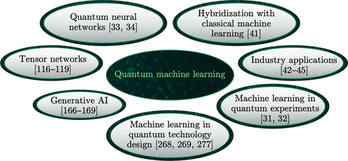
In this review, we outlined the hot topics of interplay between promising artificial intelligence methods and modern quantum computing. These topics are predominantly associated with the limited capabilities of NISQ era quantum computers and use a variety of variational algorithms, such as variational eigensolver and quantum approximate optimisation algorithm, respectively. A special place in our review is given to so-called quantum neural networks, which represent new QML models whose parameters are updated classically and may be used within quantum-classical training algorithms for variational circuits. In this sense, we discussed promising hybrid information processing methods that use both classical ML algorithms and quantum devices. The training procedure proposes data providing to the quantum model, calculating an objective (loss) value, and then adapting the QNN parameters. Thus, the whole procedure represents a hybrid quantum-classical algorithm. In this work, we discuss another possible application for hybrid computation, that may use classical-quantum convolutional neural network designed for resolving speed up of random walks on chosen graphs. Our approach is based on training CQCNN, which learns to extract feature vectors from graph adjacency matrices combined with a decoherence parameter. We have shown that even without any decoherence, in general the speedup of random walks essentially depends on topological properties of the graph, i.e. on adjacency matrix peculiarities. Our findings open new perspectives in quantum-classical algorithms, which explore random walks as subroutines.

Acknowledgments

A.P.A acknowledges support from the Goszadanie No. 2019-1339 project of the Ministry of Science and Higher Education of Russian Federation. R.-K.L. is partially supported by the National Science and Technology Council of Taiwan (No. 110-2123-M-007-002).

Disclosure statement

No potential conflict of interest was reported by the author(s).

Additional information

Funding

This work was supported by the Goszadanie.

Notes

1. Sometimes referred to as Occam’s factor [377].

2. Some alternative approaches exist known as gradient-free optimisation methods [378].

3. This is subject to the input methodology. Normally, a digital computer is used to set up the quantum circuit, in which case the learning is still fully digital.

4. Formally, when the variational architecture of a quantum circuit nears a 1-design [379].

5. ZX calculus is a graphical language in quantum information theory [186,380,381].

6. For an exhaustive list of complexity measures see [75]

7. It is noteworthy that Ref. [382] showed that some models have a higher generalisation ability despite overfitting.

8. Apart from performance considerations, this also provided an effective way to avoid barren plateaus described in Sec 2.2.5.

9. Notably the first photonic continuous-variable policy network was introduced in Ref. [383].

10. Other examples include quantum federated (distributed) learning (QFL) [384]. Notably, for the latter, Ref. [385] proposed the first model of distributed secure quantum machine learning.

11. Ref. [386] uses reinforcement learning (DPPO) to design the optimal path of quantum imaginary time evolution, which can always achieve an efficient find an efficient quantum circuit.

12. Recall quantifies the fraction of correct predictions in a particular class, whereas precision identifies the fraction of a particular class predictions that turned out to be correct.

References

- Ahmed KN. Potential of cognitive computing and cognitive systems. Open Eng. 2015;5:75–51.
- Friedemann M, Floerkemeier C. From the internet of computer to the inter- net of things (in German). Informatik-Spektrum. 2010;33:107.
- Guleva V, Shikov E, Bochenina K, et al. Emerging complexity in distributed intelligent systems. Entropy. 2020;22:1437.
- Mittal M, Shah RR, Roy S. Cognitive computing for human-robot interaction principles and practices. Cambridge, Massachusetts: Elsevier; 2021.
- Johnston ER, Harrigan N, Gimeno-Segovia M. Programming quantum computers. essential algorithms and code samples. Sebastopol, California, USA: O’Reilly Media, Inc; 2019.
- Khrennikov A. Ubiquitous quantum structure: from psychology to finances. 7.2 ed. Berlin (Heidelberg): Springer; 2010.
- Michael AN, Isaac L. Chuang. In: Quantum computation and quantum information: 10th anniversary edition. Cambridge, England: Cambridge University Press; 2011:702.
- Jack DH. Quantum computing: an applied approach. Berlin/Heidelberg, Germany: Springer; 2019.
- Feynman RP. Simulating physics with computers. International Journal of Theoretical Physics. 1982;21:467–488.
- Manin Y. Computable and uncomputable. Moscow,USSR: Sovetskoye Radio; 1980.
- Ladd TD, Jelezko F, Laflamme R, et al. Quantum computers. Nature. 2010;464:45–53.
- Preskill J. Quantum computing in the NISQ era and beyond. Quantum. 2018;2:79.
- Harrow A, Montanaro A. Quantum computational supremacy. Nature. 2017;549:203.
- Arute F, Arya K, Babbush R, et al. Quantum supremacy using a programmable superconducting processor. Nature. 2019;574:505.
- Perelshtein MR, Pakhomchik AI, Melnikov AA, et al. Solving large-scale linear systems of equations by a quantum hybrid algorithm. Annalen der Physik. 2022;534:2200082.
- Gottesman D. Technical perspective: deciphering errors to reduce the cost of quantum computation. Commun ACM. 2021;64:105.
- Terhal BM. Quantum error correction for quantum memories. Reviews of Modern Physics. 2015;87:307.
- Choi V. Minor-embedding in adiabatic quantum computation: II. minor-universal graph design. Quantum Information Processing. 2011;10:343.
- Hopfield J. Neural networks and physical systems with emergent collective computational abilities. Proceedings of the National Academy of Sciences. 1982;79:2554.
- Kendall JD, Kumar S. The building blocks of a brain-inspired computer. Applied Physics Reviews. 2020;7:011305.
- Biamonte J, Wittek P, Pancotti N, et al. Quantum machine learning. Nature. 2017;549:195–202.
- Schuld M, Sinayskiy I, Petruccione F. An introduction to quantum machine learning. Contemporary Physics. 2015;56:172–185.
- Dunjko V, Briegel HJ. Machine learning & artificial intelligence in the quantum domain: a review of recent progress. Reports on Progress in Physics. 2018;81:074001.
- Carleo G, Cirac I, Cranmer K, et al. Machine learning and the physical sciences. Rev Mod Phys. 2019;91:045002.
- Harrow AW, Hassidim A, Lloyd S. Quantum algorithm for linear systems of equations. Phys Rev Lett. 2009;103:150502.
- Aïmeur E, Brassard G, Gambs S. Quantum clustering algorithms. In ICML ’07: Proceedings of the 24th international conference on Machine learning, Corvallis, Oregon, USA; 2007. p. 1–8.
- Lloyd S, Mohseni M, Rebentrost P. Quantum principal component analysis. Nat Phys. 2014;10:631–633.
- Rebentrost P, Mohseni M, Lloyd S. Quantum support vector machine for big data classification. Phys Rev Lett. 2014;113:130503.
- Farhi E, Goldstone J, Gutmann S. A quantum approximate optimization algorithm. arXiv:1411.4028, 2014.
- Peruzzo A, McClean J, Shadbolt P, et al. A variational eigenvalue solver on a photonic quantum processor. Nat Commun. 2014 07;5:7.
- Krenn M, Malik M, Fickler R, et al. Automated search for new quantum experiments. Phys Rev Lett. 2016;116:090405.
- Melnikov AA, Poulsen Nautrup H, Krenn M, et al. Active learning machine learns to create new quantum experiments. Proc Natl Acad Sci USA. 2018;115:1221–1226.
- Farhi E, Neven H. Classification with quantum neural networks on near term processors. arXiv:1802.06002, 2018.
- Cong I, Choi S, Lukin MD. Quantum convolutional neural networks. Nat Phys. 2019;15:1273–1278.
- Fösel T, Tighineanu P, Weiss T, et al. Reinforcement learning with neural networks for quantum feedback. Phys Rev X. 2018;8:031084.
- Poulsen Nautrup H, Delfosse N, Dunjko V, et al. Optimizing quantum error correction codes with reinforcement learning. Quantum. 2019;3:215.
- Jerbi S, Gyurik C, Marshall S, et al. Parametrized quantum policies for reinforcement learning. Adv Neural Inf Process Syst. 2021;34:28362–28375.
- Saggio V, Asenbeck BE, Hamann A, et al. Experimental quantum speed-up in reinforcement learning agents. Nature. 2021;591:229–233, 03.
- Melnikov AA, Fedichkin LE, Alodjants A. Predicting quantum advantage by quantum walk with convolutional neural networks. New J Phys. 2019;21:125002.
- Melnikov AA, Fedichkin LE, Lee R-K, et al. Machine learning transfer efficiencies for noisy quantum walks. Adv Quantum Technol. 2020;3:1900115.
- Perelshtein M, Sagingalieva A, Pinto K, et al. Practical application-specific advantage through hybrid quantum computing. arXiv:2205.04858, 2022.
- Alcazar J, Leyton-Ortega V, Perdomo-Ortiz A. Classical versus quantum models in machine learning: insights from a finance application. Mach Learn Sci Technol. 2020;1:035003.
- Batra K, Zorn KM, Foil DH, et al. Quantum machine learning algorithms for drug discovery applications. J Chem Inf Model. 2021;61:2641–2647.
- Sagingalieva A, Kurkin A, Melnikov A, et al. Hyperparameter optimization of hybrid quantum neural networks for car classification. arXiv:2205.04878, 2022.
- Sagingalieva A, Kordzanganeh M, Kenbayev N, et al. Hybrid quantum neural network for drug response prediction. arXiv:2211.05777, 2022.
- DeBenedictis E. A future with quantum machine learning. Computer. 2018;51:68.
- Sajjan M, Junxu L, Selvarajan R, et al. Quantum machine learning for chemistry and physics. Chem Soc Rev. 2022;51:6475.
- Wei M, Liu Z, Kudyshev ZA, et al. Deep learning for the design of photonic structures. Nat Photonics. 2021;15:77.
- Chen Z, Segev M. Highlighting photonics: looking into the next decade. eLight. 2021;1:2.
- Ciliberto C, Herbster M, Ialongo AD, et al. Quantum machine learning: a classical perspective. Proc R Soc A. 2018;474:20170551.
- Zhang Y, Ni Q. Recent advances in quantum machine learning. Quantum Engineering. 2020;2:e34.
- Allcock J, Zhang S. Quantum machine learning. Nat Sci Rev. 2019;6:26.
- Martín-Guerrero JD, Lamata L. Quantum machine learning: a tutorial. Neurocomputing. 2022;470:457.
- Vervoort L, Melnikov AA, Chauhan M, et al. Artificial consciousness, superintelligence and ethics in robotics: how to get there? Mind and Matter. 2021;19:7–43.
- Vervoort L, Shevlin H, Melnikov A, et al. Deep learning applied to scientific discovery: a hot interface with philosophy of science. pittphilsci:19676. 2021. http://philsci-archive.pitt.edu/19676.
- Karagiorgi G, Kasieczka G, Kravitz S, et al. Machine learning in the search for new fundamental physics. Nat Rev Phys. 2022;4:399.
- Abbott RR, Abbott TD, Abraham S, et al. Observation of gravitational waves from two neutron star–black hole coalescences. Astrophys J Lett. 2021;915:L5.
- Vajente G. Data mining and machine learning improve gravitational-wave detector sensitivity. Phys Rev D. 2022;105:102005.
- McClean JR, Romero J, Babbush R, et al. The theory of variational hybrid quantum-classical algorithms. New J Phys. 2016;02;18:023023.
- Zhou L, Wang S-T, Choi S, et al. Quantum approximate optimization algorithm: performance, mechanism, and implementation on near-term devices. Phys Rev X. 2020;10:021067.
- Cerezo M, Arrasmith A, Babbush R, et al. Variational quantum algorithms. Nat Rev Phys. 2021;3:625–644.
- Deshpande A, Melnikov A. Capturing symmetries of quantum optimization algorithms using graph neural networks. Symmetry. 2022;14:2593.
- Kordzanganeh M, Sekatski P, Fedichkin L, et al. An exponentially-growing family of universal quantum circuits. arXiv:2212.00736, 2022.
- Lloyd S. Least squares quantization in PCM. IEEE Trans Inf Theory. 1982;28:129–137.
- Bacila M, Adrian R, Ioan M. Prepaid telecom customer segmentation using the K-Mean algorithm. Analele Univ din Oradea. 2012;07;21:1112–1118.
- Zulfadhilah M, Prayudi Y, Riadi I. Cyber profiling using log analysis and k-means clustering a case study higher education in Indonesia. Int J Adv Comput Sci Appl. 2016;7:430–435.
- Alejandro LG. Numerical Methods for Physics. 2nd Edition ed. New york: Prentice-Hall; 1999.
- Dai Z, Yuchen Z, Aya L, et al. The application of machine learning in bank credit rating prediction and risk assessment. In 2021 IEEE 2nd International Conference on Big Data, Artificial Intelligence and Internet of Things Engineering (ICBAIE), Nanchang, China, 986–989, 2021.
- Chunming X, Scott AJ. Machine learning and complex biological data. Genome Biol. 2019;20:76.
- Berner C, Brockman G, Chan B, et al. Dota 2 with large scale deep reinforcement learning. arXiv:1912.06680, 2019.
- Jiang Z, Dixing X, Liang J. A deep reinforcement learning framework for the financial portfolio management problem. arXiv:1706.10059, 2017.
- Maggiori E, Tarabalka Y, Charpiat G, et al. High-resolution image classification with convolutional networks. In 2017 IEEE International Geoscience and Remote Sensing Symposium (IGARSS), Fort Worth, United States; 2017. p. 5157–5160.
- Feng L, Zhang H, Xu H, et al. Mask dino: towards a unified transformer-based framework for object detection and segmentation. arXiv:2206.02777, 2022.
- Maddox WJ, Benton G, Gordon Wilson A. Rethinking parameter counting in deep models: effective dimensionality revisited. arXiv. 2020;2003:02139.
- Abbas A, Sutter D, Figalli A, et al. Effective dimension of machine learning models. arXiv. 2021;2112:04807.
- Iandola FN, Han S, Moskewicz MW, et al. SqueezeNet: AlexNet-level accuracy with 50x fewer parameters and less than 0.5MB model size. arXiv. 2016;1602:07360.
- Abdel Magid S, Petrini F, Dezfouli B. Image classification on iot edge devices: profiling and modeling. Cluster Comput. 2020;23:1025–1043.
- Ramesh A, Dhariwal P, Nichol A, et al. Hierarchical text-conditional image generation with clip latents. arXiv. 2022;2204:06125.
- Rae JW, Borgeaud S, Cai T, et al. Scaling language models: methods, analysis and insights from training gopher. arXiv. 2021;2112:11446.
- Brown T, Mann B, Ryder N, et al. Language models are few-shot learners. arXiv. 2020;2005:14165.
- Desislavov R, Martínez-Plumed F, Hernández-Orallo J. Compute and energy consumption trends in deep learning inference. arXiv. 2021;2109:05472.
- Sevilla J, Villalobos P. Parameter counts in machine learning - AI alignment forum. 06 2021. https://towardsdatascience.com/parameter-counts-in-machine-learning-a312dc4753d0
- Strubell E, Ganesh A, McCallum A. Energy and policy considerations for deep learning in NLP. arXiv. 2019;1906:02243.
- Gordon EM. Cramming more components onto integrated circuits, reprinted from electronics, volume 38, 8, April 19, 1965, pp.114 ff. IEEE Solid-State Circuits Society Newsletter. 2006;11:33–35.
- Burg D, Jesse HA. Moore’s law revisited through intel chip density. PLOS ONE. 2021;16:1–18.
- Amodei D, Hernandez D. AI and compute. 2018 [cited 2023 Jan 14]. Available from: https://openai.com/blog/ai-and-compute/
- Sevilla J, Heim L, Anson H, et al. Compute trends across three eras of machine learning. arXiv. 2022;2202:05924.
- Verhulst M, Leonard JS. The foundations of statistics. Revue économique. 1956;11;7:1042.
- Tversky A, Kahneman D. Extensional versus intuitive reasoning: the conjunction fallacy in probability judgment. Psychol Rev. 1983;90:293–315.
- Tversky A, Shafir E. The disjunction effect in choice under uncertainty. Psychol Sci. 1992;09;3:305–310.
- Emmanuel MP, Jerome RB. A quantum probability explanation for violations of ‘rational’ decision theory Proceedings of the Royal Society B. 2009;276:2171–2178 .
- Lewis M. Towards logical negation for compositional distributional semantics. arXiv. 2020;2005:04929.
- Lewis M. Quantum computing and cognitive simulation chapter. In: Quantum computing in the arts and humanities. Berlin/Heidelberg, Germany: Springer; 2022.
- Coecke B, Sadrzadeh M, Clark S. Mathematical foundations for a compositional distributional model of meaning. arXiv. 2010;1003:4394.
- David JCM. Information theory, inference, and learning algorithms. Cambridge, England: Cambridge University Press, (Imp, 7.2 edition); 2003.
- Schuld M, Petruccione F. Supervised learning with quantum computers. Berlin/Heidelberg, Germany: Cham Springer International Publishing; 2018.
- Benedetti M, Lloyd E, Sack S, et al. Parameterized quantum circuits as machine learning models. Quantum Sci Technol. 2019;11;4:043001.
- Schuld M. Supervised quantum machine learning models are kernel methods. arXiv. 2021;2101:11020.
- Lloyd S, Schuld M, Ijaz A, et al. Quantum embeddings for machine learning. arXiv. 2020;2001:03622.
- Kyriienko O, Paine AE, Elfving VE. Solving nonlinear differential equations with differentiable quantum circuits. Phys Rev A. 2021;103:1–22/052416.
- Schuld M, Bocharov A, Svore K, Wiebe N. Circuit-centric quantum classifiers. Phys Rev A. 2020;101:032308.
- Wiebe N. Key questions for the quantum machine learner to ask themselves. New J. Phys. 2020;7;22(9):091001.
- LaRose R, Coyle B. Robust data encodings for quantum classifiers. Phys Rev A. 2020;102:032420.
- Javier Gil Vidal F, Oliver Theis D. Input redundancy for parameterized quantum circuits. Front Phys. 2020;8:297.
- Schuld M, Sweke R, Meyer J. Effect of data encoding on the expressive power of variational quantum-machine-learning models. Phys Rev A. 2021;103:1–12/032430.
- Larocca M, Nathan J, García-Martín D, et al. Theory of overparametrization in quantum neural networks. arXiv. 2021;2109:11676.
- McClean JR, Boixo S, Smelyanskiy VN, et al. Barren plateaus in quantum neural network training landscapes. Nat Commun. 2018;9:11.
- Templates — pennylane 0.23.1 documentation.
- SoftwareCorporation MSC. Quantum Convolutional Neural Network — TensorFlow Quantum. [cited 2023 Jan14]. Available from: https://www.tensorflow.org/quantum/tutorials/qcnn
- Machine learning tutorials — qiskit machine learning 0.4.0 documentation. [cited 2023 Jan 14]. Available from: https://qiskit.org/documentation/machine-learning/tutorials/index.html
- Kandala A, Mezzacapo A, Temme K, et al. Hardware-efficient variational quantum eigensolver for small molecules and quantum magnets. Nature. 2017;;549:242–246.
- Shepherd D, Michael JB. Temporally unstructured quantum computation. Proceedings of the Royal Society A. 2009;465:1413–1439.
- Oseledets IV, Tyrtyshnikov EE. Breaking the curse of dimensionality, or how to use svd in many dimensions. SIAM J Sci Comput. 2009;31:3744–3759.
- Douce T, Markham D, Kashefi E, et al. Continuous-variable instantaneous quantum computing is hard to sample. Phys Rev Lett. 2017;118:1–6/070503.
- Havlíček V, Córcoles AD, Temme K, et al. Supervised learning with quantum-enhanced feature spaces. Nature. 2019;567:209–212.
- Biamonte J, Bergholm V. Tensor networks in a nutshell. arXiv. 2017;1708:00006.
- Michael LW, DAguanno G. Tree-tensor-network classifiers for machine learning: from quantum inspired to quantum assisted. Phys Rev A. 2021;104:1–23/042408.
- Singh Bhatia A, Kaur Saggi M, Kumar A, et al. Matrix product state based quantum classifier. arXiv. 2019;1905:01426.
- Kardashin A, Uvarov A, Biamonte J. Quantum machine learning tensor network states. Front Phys. 2021;8 1–6/586374 .
- Gruslys A, Munos R, Danihelka I, et al. Memory-efficient backpropagation through time. arXiv. 2016;1606:03401.
- Rumelhart DE, Hinton GE, Williams RJ. Learning representations by back-propagating errors. Nature. 1986;10;323:533–536.
- Izaac J. Quantum gradients with backpropagation - PennyLane . [cited 2023 Jan 14]. Available from: https://pennylane.ai/qml/demos/tutorial_backprop.html
- Bergholm V, Izaac J, Schuld M, et al. PennyLane: automatic differentiation of hybrid quantum-classical computations. arXiv. 2018;1811:04968.
- Schuld M, Bergholm V, Gogolin C, et al. Evaluating analytic gradients on quantum hardware. Phys Rev A. 2019;99:1–7/032331.
- Gavin EC. Gradients of parameterized quantum gates using the parameter-shift rule and gate decomposition. arXiv. 2019;1905:13311.
- Banchi L, Gavin EC. Measuring analytic gradients of general quantum evolution with the stochastic parameter shift rule. Quantum. 2021;5:01.
- Kottmann JS, Anand A, Aspuru-Guzik A. A feasible approach for automatically differentiable unitary coupled-cluster on quantum computers. Chem Sci. 2021;12:3497–3508.
- Gil Vidal J, Oliver Theis D. Calculus on parameterized quantum circuits. arXiv. 2018;1812:06323.
- Izmaylov AF, Lang RA, Yen T-C. Analytic gradients in variational quantum algorithms: algebraic extensions of the parameter-shift rule to general unitary transformations. Phys Rev A. 2021;104:12.
- Mari A, Bromley TR, Killoran N. Estimating the gradient and higher-order derivatives on quantum hardware. Phys Rev A. 2021;103:01.
- Kyriienko O, Vincent EE. Generalized quantum circuit differentiation rules. Phys Rev A. 2021;104:1–23/010313.
- Wierichs D, Izaac J, Wang C, et al. General parameter-shift rules for quantum gradients. Quantum. 2022;6:677, 03.
- Izaac J. Pennylaneai/qml, 06 2022.
- Jones T, Gacon J. Efficient calculation of gradients in classical simulations of variational quantum algorithms. arXiv. 2020;2009:02823.
- Wiersema R, Killoran N. Optimizing quantum circuits with Riemannian gradient flow. arXiv. 2022;2202:06976.
- N Pérez-Salinas A, Cervera-Lierta A, Gil-Fuster E, et al. Data re-uploading for a universal quantum classifier. Quantum. 2020;4:226.
- Biamonte J. Universal variational quantum computation. Phys Rev A. 2021;103:L030401.
- Hornik K, Stinchcombe M, White H. Multilayer feedforward networks are universal approximators. Neural Networks. 1989;2:359–366.
- Andrew Arrasmith MC, Czarnik P, Cincio L, et al. Effect of barren plateaus on gradient-free optimization. Quantum. 2021;10;5:558.
- Wang S, Enrico Fontana MC, Sharma K, et al. Noise-induced barren plateaus in variational quantum algorithms. Nat Commun. 2021;12:11.
- Skolik A, McClean JR, Mohseni M, et al. Layerwise learning for quantum neural networks. Quantum Mach Intelligence. 2021;3:01.
- Cerezo M, Sone A, Volkoff T, et al. Cost function dependent barren plateaus in shallow parametrized quantum circuits. Nat Commun. 2021;12:03.
- Holmes Z, Kunal Sharma MC, Patrick JC. Connecting ansatz expressibility to gradient magnitudes and barren plateaus. PRX Quantum. 2022;3:1–23/010313.
- Volkoff T, Coles PJ. Large gradients via correlation in random parameterized quantum circuits. Quantum Sci Technol. 2021;6:025008.
- Grant E, Wossnig L, Ostaszewski M, et al. An initialization strategy for addressing barren plateaus in parametrized quantum circuits. Quantum. 2019;3:12.
- Zhang K, Hsieh M-H, Liu L, et al. Toward trainability of quantum neural networks. arXiv. 2020;2011:06258.
- Arthur Pesah MC, Wang S, Volkoff T, et al. Absence of barren plateaus in quantum convolutional neural networks. Phys Rev X. 2021;11:041011.
- Zhao C, Gao X-S. Analyzing the barren plateau phenomenon in training quantum neural networks with the ZX-calculus. Quantum. 2021;5:466.
- Han Z-Y, Wang J, Fan H, et al. Unsupervised generative modeling using matrix product states. Phys Rev X. 2018;8:031012.
- Ortiz Marrero C, Kieferová M, Wiebe N. Entanglement-induced barren plateaus. PRX Quantum. 2021;2:040316.
- Schuld M, Killoran N. Quantum machine learning in feature Hilbert spaces. Phys Rev Lett. 2019;122:040504.
- Boser BE, Guyon IM, Vapnik VN. A training algorithm for optimal margin classifiers. In Proceedings of the Fifth Annual Workshop on Computational Learning Theory, COLT ’92, 144–152, New York, NY, USA, 1992. Association for Computing Machinery.
- Huang H-Y, Broughton M, Mohseni M, et al. Power of data in quantum machine learning. Nat Commun. 2021;12:05.
- Bayes T. An essay towards solving a problem in the doctrine of chances. by the late rev. Mr. Bayes communicated by Mr. Price, in a letter to John canton. Philos Trans R Soc London. 1763;53:370–418, 12.
- Graves A. Practical variational inference for neural networks. In: Shawe-Taylor J, Zemel R, Bartlett P, et al., editors. Advances in neural information processing systems. Vol. 24. Granada, Spain: Curran Associates, Inc; 2011. p. 2348–2356.
- Blundell C, Cornebise J, Kavukcuoglu K, et al. Weight uncertainty in neural networks. arXiv. 2015;1505:05424.
- Hao Low G, Yoder TJ, Chuang IL. Quantum inference on Bayesian networks. Phys Rev A. 2014;89:06.
- Borujeni SE, Nannapaneni S, Nguyen NH, et al. Quantum circuit representation of Bayesian networks. Expert Syst Appl. 2021;08;176:114768.
- Robert RT. Quantum Bayesian nets. Int J Modern Phys B. 1995;01;09:295–337.
- Benedetti M, Coyle B, Fiorentini M, et al. Variational inference with a quantum computer. Phys Rev Appl. 2021;16:044057.
- Cheng S, Chen J, Wang L. Information perspective to probabilistic modeling: Boltzmann machines versus born machines. Entropy. 2018;20:1–14/583.
- Coyle B, Mills D, Danos V, et al. The Born supremacy: quantum advantage and training of an Ising Born machine. Npj Quantum Inf. 2020;6:60.
- Liu J-G, Wang L. Differentiable learning of quantum circuit Born machines. Phys Rev A. 2018;98:062324.
- Čepaitė I, Coyle B, Kashefi E. A continuous variable Born machine. arXiv. 2020;2011:00904.
- Leyton-Ortega V, Perdomo-Ortiz A, Perdomo O. Robust implementation of generative modeling with parametrized quantum circuits. Quantum Mach Intelligence. 2021;3:17.
- Hamilton KE, Dumitrescu EF, Pooser RC. Generative model benchmarks for superconducting qubits. Phys Rev A. 2019;99:062323.
- Gao X, Anschuetz ER, Sheng-Tao Wang JIC, et al. Enhancing generative models via quantum correlations. arXiv. 2021;2101:08354.
- Benedetti M, Garcia-Pintos D, Perdomo O, et al. A generative modeling approach for benchmarking and training shallow quantum circuits. Npj Quantum Inf. 2019;5:45.
- Kendall A, Gal Y. What uncertainties do we need in Bayesian deep learning for computer vision? arXiv. 2017;1703:04977.
- Vapnik VN, Chervonenkis AY. On the uniform convergence of relative frequencies of events to their probabilities. Theory of Probability & Its Applications. 1971;16:264–280.
- Peter LB, Mendelson S. Rademacher and Gaussian complexities: risk bounds and structural results. Journal of Machine Learning Research. 2002;3:463–482.
- Berezniuk O, Figalli A, Ghigliazza R, et al. A scale-dependent notion of effective dimension. arXiv. 2020;2001:10872.
- Caro MC, Gil-Fuster E, Jakob Meyer J, et al. Encoding-dependent generalization bounds for parametrized quantum circuits. Quantum. 2021;5:582.
- Abbas A, Sutter D, Zoufal C, et al. The power of quantum neural networks. arXiv. 2020;2011:00027.
- Sim S, Johnson PD, Aspuru‐Guzik A. Expressibility and entangling capability of parameterized quantum circuits for hybrid quantum‐classical algorithms. Adv Quantum Technol. 2019;2:1900070.
- Bouland A, Fefferman B, Nirkhe C, et al. On the complexity and verification of quantum random circuit sampling. Nat Phys. 2019;15:159–163.
- Du Y, Hsieh M-H, Liu T, et al. Expressive power of parametrized quantum circuits. Phys Rev Res. 2020;2:033125.
- Matthias CC, Datta I. Pseudo-dimension of quantum circuits. Quantum Mach Intelligence. 2020;2:14.
- Holmes Z, Kunal Sharma MC, Coles PJ. Connecting ansatz expressibility to gradient magnitudes and barren plateaus. arXiv. 2021;2101:02138.
- Caro MC, Hsin-Yuan Huang MC, Sharma K, et al. Generalization in quantum machine learning from few training data. arXiv. 2021;2111:05292.
- QMware — the first global quantum cloud,
- Kordzanganeh M, Buchberger M, Povolotskii M, et al. Benchmarking simulated and physical quantum processing units using quantum and hybrid algorithms. arXiv. 2022;2211:15631.
- sklearn.datasets.make_circles, Accessed 2022-06-17.
- Harrison D, Rubinfeld D. Hedonic housing prices and the demand for clean air. J Environ Econ Manage. 1978;03;5:81–102.
- Krause J, Stark M, Deng J, et al. 3D object representations for fine-grained categorization. In 2013 IEEE International Conference on Computer Vision Workshops, Sydney, Australia; 2013. p. 554–561.
- Coecke B, Duncan R. A graphical calculus for quantum observables. E-Preprint. 2007 [cited 2023 Jan 14]. Available from: https://www.researchgate.net/profile/Bob-Coecke/publication/267999929_A_graphical_calculus_for_quantum_observables/links/546dd6bc0cf2193b94c5d1f8/A-graphical-calculus-for-quantum-observables.pdf
- Petz D, Ghinea C. Introduction to quantum Fisher information. arXiv. 2010;1008:2417.
- Liu J, Yuan H, Xiao-Ming L, et al. Quantum Fisher information matrix and multiparameter estimation. J Phys A. 2019;53:11.
- Kordzanganeh M, Utting A, Scaife A. Quantum machine learning for radio astronomy. arXiv. 2021;2112:02655.
- Junde L, Topaloglu R, Ghosh S. Quantum generative models for small molecule drug discovery. arXiv. 2021;2101:03438.
- G De Las C, Dür W, Van den Nest M, et al. Quantum algorithms for classical lattice models. New J Phys. 2011;13:093021.
- Lamata L. Quantum machine learning and quantum biomimetics: a perspective. Mach Learn Sci Technol. 2020;1:033002.
- Nannicini G. Performance of hybrid quantum-classical variational heuristics for combinatorial optimization. Phys Rev E. 2019;99:013304.
- Terashi K, Kaneda M, Kishimoto T, et al. Event classification with quantum machine learning in high-energy physics. Computing and Software for Big Science. 2021;5:2.
- Guan W, Perdue G, Pesah A, et al. Quantum machine learning in high energy physics. Mach Learn Sci Technol. 2021;2:011003.
- Coyle B, Henderson M, Chan Jin Le J, et al. Quantum versus classical generative modelling in finance. Quantum Sci Technol. 2021;6:024013.
- Emmanoulopoulos D, Dimoska S. Quantum machine learning in finance: time series forecasting. arXiv. 2022;2202:00599.
- Pistoia M, Farhan Ahmad S, Ajagekar A, et al. Quantum machine learning for finance. arXiv. 2021;2109:04298.
- Gao X, Zhang Z-Y, Duan L-M. A quantum machine learning algorithm based on generative models. Sci Adv. 2018;4:eaat9004.
- Benedetti M, Realpe-Gómez J, Perdomo-Ortiz A. Quantum-assisted Helmholtz machines: a quantum–classical deep learning framework for industrial datasets in near-term devices. Quantum Sci Technol. 2018;3:034007.
- Johri S, Debnath S, Mocherla A, et al. Nearest centroid classification on a trapped ion quantum computer. arXiv. 2020;2012:04145.
- Shingu Y, Seki Y, Watabe S, et al. Boltzmann machine learning with a variational quantum algorithm. Phys Rev A. 2021;104:032413.
- Lloyd S, Weedbrook C. Quantum generative adversarial learning. Phys Rev Lett. 2018;121:040502.
- Dallaire-Demers P-L, Killoran N. Quantum generative adversarial networks. Phys Rev A. 2018;98:012324.
- Benedetti M, Grant E, Wossnig L, et al. Adversarial quantum circuit learning for pure state approximation. New J Phys. 2019;21:043023.
- Zeng J, Yufeng W, Liu J-G, et al. Learning and inference on generative adversarial quantum circuits. Phys Rev A. 2019;99:052306.
- Rudolph MS, Bashige Toussaint N, Katabarwa A, et al. Generation of high-resolution handwritten digits with an ion-trap quantum computer. arXiv. 2020;2012:03924.
- Situ H, Zhimin H, Wang Y, et al. Quantum generative adversarial network for generating discrete distribution. Inf Sci. 2020;538:193–208.
- Herr D, Obert B, Rosenkranz M. Anomaly detection with variational quantum generative adversarial networks. Quantum Sci Technol. 2021;6:045004.
- Huang H-L, Du Y, Gong M, et al. Experimental quantum generative adversarial networks for image generation. Phys Rev Appl. 2021;16:024051.
- Stein SA, Baheri B, Chen D, et al. QuGAN: a quantum state fidelity based generative adversarial network. 2021 IEEE International Conference on Quantum Computing and Engineering (QCE), Broomfield, CO, USA, 2021;00:71–81.
- Bausch J. Recurrent quantum neural networks. In: Larochelle H, Ranzato M, Hadsell R, et al., editors. Advances in neural information processing systems. Vol. 33. New York, USA: Curran Associates, Inc; 2020. p. 1368–1379.
- Takaki Y, Mitarai K, Negoro M, et al. Learning temporal data with a variational quantum recurrent neural network. Phys Rev A. 2021;103:052414.
- Henderson M, Shakya S, Pradhan S, et al. Quanvolutional neural networks: powering image recognition with quantum circuits. arXiv. 2019;1904:04767.
- O’Riordan LJ, Doyle M, Baruffa F, et al. A hybrid classical-quantum workflow for natural language processing. Mach Learn Sci Technol. 2020;2:015011.
- Dong D, Chen C, Hanxiong L, et al. Quantum reinforcement learning. IEEE Trans Syst Man Cybern Part B Cybern. 2008;38:1207–1220.
- Ji-An L, Dong D, Wei Z, et al. Quantum reinforcement learning during human decision-making. Nat Hum Behav. 2020;4:294–307. doi:10.1038/s41562-019-0804-2.
- Lamata L. Quantum reinforcement learning with quantum photonics. Photonics. 2021;8:33, 01.
- Khoshaman A, Vinci W, Denis B, et al. Quantum variational autoencoder. Quantum Sci Technol. 2019;4:014001.
- Aharonov D, Ta-Shma A. Adiabatic quantum state generation and statistical zero knowledge. arXiv. 2003;quant-ph:0301023.
- Berry DW, Ahokas G, Cleve R, et al. Efficient quantum algorithms for simulating sparse hamiltonians. Commun Math Phys. 2007;270:359–371.
- Leyton SK, Osborne TJ. A quantum algorithm to solve nonlinear differential equations. arXiv. 2008;0812:4423.
- Berry DW. High-order quantum algorithm for solving linear differential equations. J Phys A. 2014;47:105301.
- Berry DW, Childs AM, Ostrander A, et al. Quantum algorithm for linear differential equations with exponentially improved dependence on precision. Commun Math Phys. 2017;356:1057–1081.
- Kiani BT, De Palma G, Englund D, et al. Quantum advantage for differential equation analysis. arXiv. 2020;2010:15776.
- Andrew MacGregor Childs. PhD Thesis: Quantum Information Processing in Continuous Time Andrew MacGregor Childs. Massachusetts Institute of Technology; 2004.
- Shmoys D, Berry DW, Childs AM, et al. Exponential improvement in precision for simulating sparse Hamiltonians. Proceedings of the forty-sixth annual ACM symposium on Theory of computing, New York, USA; 2014. p. 283–292.
- Lloyd S, De Palma G, Gokler C, et al. Quantum algorithm for nonlinear differential equations. arXiv. 2020;2011:06571.
- Zionts S, Hammer (Ivanescu) PL, Rudeanu S. Boolean methods in operations research and related areas. Econometrica. 1972;07;40:777.
- Laughhunn DJ. Quadratic binary programming with application to capital-budgeting problems. Oper Res. 1970;06;18:454–461.
- McKeehan LW. A contribution to the theory of ferromagnetism. Phys Rev. 1925;26:274–279.
- Rønnow TF, Wang Z, Job J, et al. Defining and detecting quantum speedup. Science. 2014;345:420–424.
- Booth M, Berwald J, Chukwu U, et al. QCI Qbsolv delivers strong classical performance for quantum-ready formulation. arXiv. 2020;2005:11294.
- Wang X. Efficiently solve the max-cut problem via a quantum qubit rotation algorithm. arXiv. 2021;2110:08016.
- Sato I, Kurihara K, Tanaka S, et al. Quantum annealing for variational Bayes inference. arXiv. 2014;1408:2037.
- O’Gorman B, Babbush R, Perdomo-Ortiz A, et al. Bayesian network structure learning using quantum annealing. The European Physical Journal Special Topics. 2015;224:163–188.
- Wilson M, Vandal T, Hogg T, et al. Quantum-assisted associative adversarial network: applying quantum annealing in deep learning. Quantum Mach Intelligence. 2021;3:19.
- Hernández F, Díaz K, Forets M, et al. Application of quantum optimization techniques (QUBO method) to cargo logistics on ships and airplanes. In 2020 IEEE Congreso Bienal de Argentina (ARGENCON), Resistencia, Argentina; 2020. p. 1–1.
- Lambek J. The mathematics of sentence structure. Am Math Monthly. 1958;65:03.
- Lorenz R, Pearson A, Meichanetzidis K, et al. QNLP in practice: running compositional models of meaning on a quantum computer. arXiv. 2021;2102:12846.
- Meichanetzidis K, Toumi A, de Felice G, et al. Grammar-aware question-answering on quantum computers. arXiv. 2020;2012:03756.
- Coecke B, de Felice G, Meichanetzidis K, et al. Foundations for near-term quantum natural language processing. arXiv. 2012;2020:03755.
- Yeung R, Fan I, London C. lambeq, 06 2022.
- Grover L. A fast quantum mechanical algorithm for database search. arXiv. 1996;9605043:1–8.
- Liu Y, Arunachalam S, Temme K. A rigorous and robust quantum speed-up in supervised machine learning. Nat Phys. 2021;17:1–5.
- Rocco AS, Steven JG. Equivalences and separations between quantum and classical learnability. SIAM J Comput. 2004;33:1067–1092.
- Ristè D, da Silva MP, Ryan CA, et al. Demonstration of quantum advantage in machine learning. Npj Quantum Inf. 2017;3:16.
- Boixo S, Isakov SV, Smelyanskiy VN, et al. Characterizing quantum supremacy in near-term devices. Nat Phys. 2018;14:595–600.
- Schuld M, Killoran N. Is quantum advantage the right goal for quantum machine learning? arXiv. 2022;2203:01340.
- Bukov M, Day AGR, Sels D, et al. Reinforcement learning in different phases of quantum control. Phys Rev X. 2018;8:031086.
- Han X, Junning L, Liu L, et al. Generalizable control for quantum parameter estimation through reinforcement learning. Npj Quantum Inf. 2019;5:82.
- Luchnikov IA, Vintskevich SV, Grigoriev DA, et al. Machine learning non-Markovian quantum dynamics. Phys Rev Lett. 2020;124:140502.
- Schäfer F, Kloc M, Bruder C, et al. A differentiable programming method for quantum control. Mach Learn: Sci Technol. 2020;1:035009.
- Tiersch M, Ganahl EJ, Briegel HJ. Adaptive quantum computation in changing environments using projective simulation. Sci Rep. 2015;5:12874.
- Sweke R, Kesselring MS, van Nieuwenburg EPL, et al. Reinforcement learning decoders for fault-tolerant quantum computation. Mach Learn: Sci Technol. 2020;2:025005.
- Valenti A, van Nieuwenburg E, Huber S, et al. Hamiltonian learning for quantum error correction. Phys Rev Res. 2019;1:033092.
- Liu G, Chen M, Liu Y-X, et al. Repetitive readout enhanced by machine learning. Mach Learn: Sci Technol. 2020;1:015003.
- Shang Y, Albarrán-Arriagada F, Carlos Retamal J, et al. Reconstruction of a photonic qubit state with reinforcement learning. Adv Quantum Technol. 2019;2:1800074.
- Torlai G, Timar B, van Nieuwenburg EPL, et al. Integrating neural networks with a quantum simulator for state reconstruction. Phys Rev Lett. 2019;123:230504.
- Macarone Palmieri A, Kovlakov E, Bianchi F, et al. Experimental neural network enhanced quantum tomography. Npj Quantum Inf. 2020;6:20.
- Ding Y, Martín-Guerrero JD, Sanz M, et al. Retrieving quantum information with active learning. Phys Rev Lett. 2020;124:140504.
- Carleo G, Troyer M. Solving the quantum many-body problem with artificial neural networks. Science. 2017;355:602–606.
- Gao X, Duan L-M. Efficient representation of quantum many-body states with deep neural networks. Nat Commun. 2017;8:662.
- Agresti I, Viggianiello N, Flamini F, et al. Pattern recognition techniques for boson sampling validation. Phys Rev X. 2019;9:011013.
- Einstein A, Podolsky B, Rosen N. Can quantum-mechanical description of physical reality be considered complete? Phys Rev. 1935;47:777–780.
- Sekatski P, Bancal J-D, Valcarce X, et al. Device-independent quantum key distribution from generalized CHSH inequalities. Quantum. 2021;5:444.
- Canabarro A, Brito S, Chaves R. Machine learning nonlocal correlations. Phys Rev Lett. 2019;122:200401.
- Melnikov AA, Sekatski P, Sangouard N. Setting up experimental Bell tests with reinforcement learning. Phys Rev Lett. 2020;125:160401.
- Valcarce X, Sekastki P, Gouzien E, et al. Automated design of quantum optical experiments for device-independent quantum key distribution. arXiv. 2022;2209:06468.
- Hans J. Briegel and Gemma De las Cuevas. Projective simulation for artificial intelligence. Sci Rep. 2012;2:400.
- Mautner J, Makmal A, Manzano D, et al. Projective simulation for classical learning agents: a comprehensive investigation. New Gener Comput. 2015;33:69–114.
- Makmal A, Melnikov AA, Dunjko V, et al. Meta-learning within projective simulation. IEEE Access. 2016;4:2110–2122.
- Melnikov AA, Makmal A, Dunjko V, et al. Projective simulation with generalization. Sci Rep. 2017;7:14430.
- Melnikov AA, Makmal A, Briegel HJ. Benchmarking projective simulation in navigation problems. IEEE Access. 2018;6:64639–64648.
- Projective simulation Github repository. github.com/qic-ibk/projectivesimulation. Accessed: 2022-04-05.
- Cincio L, Subaşı Y, Sornborger AT, et al. Learning the quantum algorithm for state overlap. New J Phys. 2018;20:113022.
- Wallnöfer J, Melnikov AA, Dür W, et al. Machine learning for long-distance quantum communication. PRX Quantum. 2020;1:010301.
- Giese B, Amaudrut J, Köhler A-K, et al. Direct observation of hole transfer through DNA by hopping between adenine bases and by tunnelling. Nature. 2001;412:318–320.
- Lee H, Cheng Y-C, Fleming GR. Coherence dynamics in photosynthesis: protein protection of excitonic coherence. Science. 2007;316:1462–1465.
- Farhi E, Gutmann S. Quantum computation and decision trees. Phys Rev A. 1998;58:1462–1465.
- Kac M. Random walk and the theory of Brownian motion. Am Math Mon. 1947;54:369–391.
- Gräfe M, Heilmann R, Lebugle M, et al. Integrated photonic quantum walks. J Opt. 2018;18:103002.
- Motwani R, Raghavan P. Randomized algorithms. New York: Cambridge University Press; 1995.
- Grady L. Random walks for image segmentation. IEEE Trans Pattern Anal Mach Intell. 2006;28:1768–1783.
- Gkantsidis C, Milena A, Saberi MA. Random walks in peer-to-peer networks: algorithms and evaluation. Perform Eval. 2006;63:241–263.
- Aharonov Y, Davidovich L, Zagury N. Quantum random walks. Phys Rev A. 1993;48:1687–1690.
- Kempe J. Quantum random walks: an introductory overview. Contemp Phys. 2003;44:307–327.
- Bromberg Y, Lahini Y, Morandotti R, et al. Quantum and classical correlations in waveguide lattices. Phys Rev Lett. 2009;102:253904.
- Ambainis A, Bach E, Nayak A, et al. One-dimensional quantum walks. In Proceedings of the 33rd Annual ACM Symposium on Theory of Computing, STOC ’01, 37–49, New York, NY, USA, 2001. ACM.
- Solenov D, Fedichkin L. Continuous-time quantum walks on a cycle graph. Phys Rev A. 2006;73:012313.
- Melnikov AA, Fedichkin LE. Quantum walks of interacting fermions on a cycle graph. Sci Rep. 2016;6:1–13.
- Kempe J. Discrete quantum walks hit exponentially faster. Probab Theory Relat Fields. 2005;133:215–235.
- Krovi H, Todd AB. Hitting time for quantum walks on the hypercube. Phys Rev A. 2006;73:032341.
- Childs AM, Cleve R, Deotto E, et al. Exponential algorithmic speedup by a quantum walk. In Proceedings of the 35th Annual ACM Symposium on Theory of Computing, STOC ’03, 59–68, New York, NY, USA, 2003. ACM.
- Ambainis A. Quantum walks and their algorithmic applications. Int J Quantum Inf. 2003;1:507–518.
- Elias Venegas-Andraca S. Quantum walks for computer scientists, volume 1 of synthesis lectures on quantum computing. San Rafael, California, USA: Morgan & Claypool Publishers; 2008.
- Portugal R. Quantum walks and search algorithms. Berlin/Heidelberg, Germany: Springer; 2013.
- Davide Paparo G, Dunjko V, Makmal A, et al. Quantum speedup for active learning agents. Phys Rev X. 2014;4:031002.
- Chakraborty S, Novo L, Ambainis A, et al. Spatial search by quantum walk is optimal for almost all graphs. Phys Rev Lett. 2016;116:100501.
- Melnikov AA, Alodjants AP, Fedichkin LE. Hitting time for quantum walks of identical particles. In Proceedings of SPIE, International Conference on Micro- and Nano-Electronics 2018, Zvenigorod, Russia; 2019. Vol. 11022. p. 110222J.
- Kryukov A, Abramov R, Fedichkin LE, et al. Supervised graph classification for chiral quantum walks. Phys Rev A. 2022;105:022208.
- Melnikov AA, Fedichkin LE, Alodjants A. On training a classifier of hitting times for quantum walks. In AIP Conference Proceedings, Moscow, Russia. AIP Publishing LLC; 2020. Vol. 2241, p. 020029.
- Melnikov AA, Fedichkin LE, Lee R-K, et al. Deep neural networks classifying transfer efficiency in complex networks. In 2020 Opto-Electronics and Communications Conference (OECC), Taipei, Taiwan. IEEE; 2020. p. 1–3.
- Manzano D. A short introduction to the Lindblad master equation. AIP Adv. 2020;10:025106.
- Larkin AL, Ovchinnikov YN. Quantum tunnelling in a dissipative system. JETP Lett. 1983;37:382–385.
- Grabert H, Weiss U, Hanggi P. Quantum tunneling in dissipative systems at finite temperatures. Phys Rev Lett. 1984;52:2193–2196.
- Lebedev ME, Dolinina DA, Hong K-B, et al. Exciton-polariton Josephson junctions at finite temperatures. Sci Rep. 2017;7:9515.
- Hradil Z. Quantum-state estimation. Phys Rev A. 1997;55:R1561–R1564.
- Řeháček J, Hradil Z, Ježek M. Iterative algorithm for reconstruction of entangled states. Phys Rev A. 2001;63:040303.
- James DFV, Kwiat PG, Munro WJ, et al. Measurement of qubits. Phys Rev A. 2001;64:052312.
- Blume-Kohout R. Optimal, reliable estimation of quantum states. New J Phys. 2010;12:043034.
- Ježek M, Fiurášek J, Ěk Hradil Z. Quantum inference of states and processes. Phys Rev A. 2003;68:012305.
- Leonhardt U. Quantum and classical tomography with equidistant reference angles. J Mod Opt. 1997;44:2271–2280.
- Lvovsky AI, Raymer MG. Continuous-variable optical quantum-state tomography. Rev Mod Phys. 2009;81:299–332.
- Carrasquilla J, Torlai G. How to use neural networks to investigate quantum many-body physics. PRX Quantum. 2021;2:040201.
- Lvovsky AI. Iterative maximum-likelihood reconstruction in quantum homodyne tomography. J Opt B: Quantum Semiclassical Opt. 2004;6:S556–S559.
- Smolin JA, Gambetta JM, Smith G. Efficient method for computing the maximum-likelihood quantum state from measurements with additive Gaussian noise. Phys Rev Lett. 2012;108:070502.
- Granade C, Ferrie C, Flammia ST. Practical adaptive quantum tomography. New J Phys. 2017;19:113017.
- Tóth G, Wieczorek W, Gross D, et al. Permutationally invariant quantum tomography. Phys Rev Lett. 2010;105:250403.
- Flammia ST, Gross D, Liu Y-K, et al. Quantum tomography via compressed sensing: error bounds, sample complexity and efficient estimators. New J Phys. 2012;14:095022.
- Gross D, Liu Y-K, Flammia ST, et al. Quantum state tomography via compressed sensing. Phys Rev Lett. 2010;105:150401.
- Shabani A, Kosut RL, Mohseni M, et al. Efficient measurement of quantum dynamics via compressive sensing. Phys Rev Lett. 2011;106:100401.
- Riofrío CA, Gross D, Flammia ST, et al. Experimental quantum compressed sensing for a seven-qubit system. Nat Commun. 2017;8:15305.
- Cramer M, Plenio MB, Flammia ST, et al. Efficient quantum state tomography. Nat Commun. 2010;1:149.
- Lanyon BP, Maier C, Holzäpfel M, et al. Efficient tomography of a quantum many-body system. Nat Phys. 2017;13:1158.
- Carrasquilla J, Torlai G, Melko RG, et al. Reconstructing quantum states with generative models. Nat Mach Intell. 2019;1:155–161.
- Xin T, Sirui L, Cao N, et al. Local-measurement-based quantum state tomography via neural networks. Npj Quantum Inf. 2019;5:109.
- Rocchetto A, Grant E, Strelchuk S, et al. Learning hard quantum distributions with variational autoencoders. Npj Quantum Inf. 2018;4:28.
- Tiunov ES, Tiunova VV, Ulanov AE, et al. Experimental quantum homodyne tomography via machine learning. Optica. 2020;7:448–454.
- Le Roux N, Bengio Y. Representational power of restricted Boltzmann machines and deep belief networks. Neural Comput. 2008;20:1631–1649.
- Ackley DH, Hinton GE, Sejnowski TJ. A learning algorithm for Boltzmann machines*. Cogn Sci. 1985;9:147–169.
- Sehayek D, Golubeva A, Albergo MS, et al. Learnability scaling of quantum states: restricted Boltzmann machines. Phys Rev B. 2019;100:195125.
- Lohani S, Searles TA, Kirby BT, et al. On the experimental feasibility of quantum state reconstruction via machine learning. IEEE Trans Quantum Eng. 2021;2:1–10.
- Melkani A, Gneiting C, Nori F. Eigenstate extraction with neural-network tomography. Phys Rev A. 2020;102:022412.
- Hsieh H-Y, Chen Y-R, Hsun-Chung W, et al. Extract the degradation information in squeezed states with machine learning. Phys Rev Lett. 2022;128:073604.
- Krizhevsky A, Sutskever I, Hinton GE. Imagenet classification with deep convolutional neural networks. Commun ACM. 2017;60:84–90.
- Kaiming H, Zhang X, Ren S, et al. Deep residual learning for image recognition. In 2016 IEEE Conference on Computer Vision and Pattern Recognition (CVPR), Las Vegas, NV, USA; 2016. p.770–778.
- Hsieh H-Y, Ning J, Chen Y-R, et al. Direct parameter estimations from machine learning-enhanced quantum state tomography. Symmetry. 2022;14:1–10/874.
- Zhang X, Luo M, Wen Z, et al. Direct fidelity estimation of quantum states using machine learning. Phys Rev Lett. 2021;127:130503.
- Danaci O, Lohani S, Kirby BT, et al. Machine learning pipeline for quantum state estimation with incomplete measurements. Mach Learn Sci Technol. 2021;2:035014.
- Haroche S. Nobel lecture: controlling photons in a box and exploring the quantum to classical boundary. Rev Mod Phys. 2013;85:1083–1102.
- David JW. Nobel lecture: superposition, entanglement, and raising Schrodinger's cat. Rev Mod Phys. 2013;85:1103–1114.
- Gottesman D, Kitaev A, Preskill J. Encoding a qubit in an oscillator. Phys Rev A. 2001;64:012310.
- Ahmed S, Sánchez Muñoz C, Nori F, et al. Quantum state tomography with conditional generative adversarial networks. Phys Rev Lett. 2021;127:140502.
- Ahmed S, Sánchez Muñoz C, Nori F, et al. Classification and reconstruction of optical quantum states with deep neural networks. Phys Rev Res. 2021;3:033278.
- Quek Y, Fort S, Hui Khoon N. Adaptive quantum state tomography with neural networks. Npj Quantum Inf. 2021;7:105.
- Nakaji K, Yamamoto N. Quantum semi-supervised generative adversarial network for enhanced data classification. Sci Rep. 2021;11:19649.
- Haug T, Mok W-K, You J-B, et al. Classifying global state preparation via deep reinforcement learning. Mach Learn Sci Technol. 2020;2:01LT02.
- Koutný D, Motka L, Ěk Hradil Z, et al. Neural-network quantum state tomography. Phys Rev A. 2022;106:012409.
- Cha P, Ginsparg P, Felix W, et al. Attention-based quantum tomography. Mach Learn Sci Technol. 2021;3:01LT01.
- Siah Teo Y, Shin S, Jeong H, et al. Benchmarking quantum tomography completeness and fidelity with machine learning. New J Phys. 2021;23:103021.
- Navon N, Akerman N, Kotler S, et al. Quantum process tomography of a mølmer-sørensen interaction. Phys Rev A. 2014;90:010103.
- Takahashi M, Bartlett SD, Doherty AC. Tomography of a spin qubit in a double quantum dot. Phys Rev A. 2013;88:022120.
- O’Brien JL, Pryde GJ, Gilchrist A, et al. Quantum process tomography of a controlled-not gate. Phys Rev Lett. 2004;93:080502.
- Chen-Di H, Glaz B, Haile M, et al. Tomography of time-dependent quantum hamiltonians with machine learning. Phys Rev A. 2021;104:062404.
- Deville Y, Deville A. New single-preparation methods for unsupervised quantum machine learning problems. IEEE Trans Quantum Eng. 2021;2:1–24.
- Zhong H-S, Wang H, Deng Y-H, et al. Quantum computational advantage using photons. Science. 2020;370:1460–1463.
- Zhong H-S, Deng Y-H, Qin J, et al. Phase-programmable Gaussian boson sampling using stimulated squeezed light. Phys Rev Lett. 2021;127:180502.
- Aaronson S, Arkhipov A. The computational complexity of linear optics. In Proceedings of the Forty-Third Annual ACM Symposium on Theory of Computing, STOC ’11, 333–342, New York, NY, USA, 2011. Association for Computing Machinery.
- Wang J, Sciarrino F, Laing A, et al. Integrated photonic quantum technologies. Nat Photonics. 2020;14:273–284.
- Elshaari AW, Pernice W, Srinivasan K, et al. Hybrid integrated quantum photonic circuits. Nat Photonics. 2020;14:285–298.
- Duan B, Wu B, Chen J-H, et al. Deep learning for photonic design and analysis: principles and applications. Front Mater. 2022 Jan;8:791296.
- Sui X, Qiuhao W, Liu J, et al. A review of optical neural networks. IEEE Access. 2020;8:70773–70783.
- Wei M, Cheng F, Yihao X, et al. Probabilistic representation and inverse design of metamaterials based on a deep generative model with semi-supervised learning strategy. Adv Mater. 2019;31:1901111.
- Manzalini A. Complex deep learning with quantum optics. Quantum Rep. 2019;1:107–118.
- Chabaud U, Markham D, Sohbi A. Quantum machine learning with adaptive linear optics. Quantum. 2021;5:496.
- Reimer C, Kues M, Roztocki P, et al. Generation of multiphoton entangled quantum states by means of integrated frequency combs. Science. 2016;351:1176–1180.
- Kues M, Reimer C, Roztocki P, et al. On-chip generation of high-dimensional entangled quantum states and their coherent control. Nature. 2017;546:622–626.
- Kues M, Reimer C, Lukens JM, et al. Quantum optical microcombs. Nat Photonics. 2019;13:170.
- Yang Z, Jahanbozorgi M, Jeong D, et al. A squeezed quantum microcomb on a chip. Nat Commun. 2021;12:4781.
- Guidry MA, Lukin DM, Yang KY, et al. Quantum optics of soliton microcombs. Nat Photonics. 2022;16:52.
- Asavanant W, Shiozawa Y, Yokoyama S, et al. Generation of time-domain-multiplexed two-dimensional cluster state. Science. 2019;366:373–376.
- Larsen MV, Guo X, Breum CR, et al. Deterministic generation of a two-dimensional cluster state. Science. 2019;366:369–372.
- Kudyshev ZA, Shalaev VM, Boltasseva A. Machine learning for integrated quantum photonics. ACS Photonics. 2021;8:34–46.
- Krenn M, Kottmann JS, Tischler N, et al. Conceptual understanding through efficient automated design of quantum optical experiments. Phys Rev X. 2021;11:031044.
- Steinbrecher GR, Olson JP, Englund D, et al. Quantum optical neural networks. Npj Quantum Inf. 2019;5:60.
- MacKay D. Bayesian model comparison and backprop nets. In: Moody J, Hanson S, Lippmann RP, editors. NIPS'91: Proceedings of the 4th International Conference on Neural Information Processing Systems, Denver Colorado, USA; 2-5 December, 1991. Morgan Kaufmann Publishers Inc.340 Pine Street, Sixth FloorSan FranciscoCAUnited States; 1991. Vol. 4, p. 839–846.
- Larson J, Menickelly M, Wild SM. Derivative-free optimization methods. Acta Numerica. 2019;28:287–404.
- Ambainis A, Emerson J. Quantum t-designs: t-wise Independence in the quantum world. arXiv. 2007;quant-ph:0701126.
- Coecke B. Quantum picturalism. Contemp Phys. 2010;51:59–83.
- Coecke B, Duncan R. Interacting quantum observables: categorical algebra and diagrammatics. New J Phys. 2011;13:043016.
- Peters, Evan, Schuld, Maria Generalization despite overfitting in quantum machine learning models; 2022. arXiv:2209.05523. doi:10.48550/arXiv.2209.05523.
- Nagy, D., Tabi, Z., Hága, P., Kallus, Z. and Zimborás, Z, 2021. Photonic quantum policy learning in OpenAI Gym. 2021 IEEE International Conference on Quantum Computing and Engineering (QCE), Broomfield, Colorado, USA. IEEE. p. 123–129.
- Mahdi Chehimi and Walid Saad. Quantum federated learning with quantum data. ICASSP 2022 - 2022 IEEE International Conference on Acoustics, Speech and Signal Processing (ICASSP), Singapore; 2022. p. 8617–8621.
- Yu-Bo Sheng and Lan Zhou. Distributed secure quantum machine learning. Science Bulletin. 2017;62(14):1025–1029.
- Chenfeng Cao, Zheng An, Shi-Yao Hou, D. L. Zhou, and Bei Zeng. Quantum imaginary time evolution steered by reinforcement learning. Communications Physics; 5(1):2022.