Using rainfall measures to evaluate hydrologic performance of green infrastructure systems under climate change

ABSTRACT

As climate change alters precipitation patterns, stakeholders will need to understand how performance of green stormwater infrastructure (GSI) could change in response. As an alternative to using on-site monitoring, which may not always feasible, we propose that changes in performance could be tracked using annual rainfall measures (e.g., maximum daily rainfall per year). We estimated performance of GSI in 17 U.S. cities using rainfall measures by establishing linear relationships with specific performance metrics (e.g., frequency of discharge). Prediction accuracy was evaluated in 2 cities for the period 2020 to 2060 by comparing performance predicted from rainfall trends from regional climate models (RCMs) with simulated performance in SWMM using the same RCMs as input. Findings suggest that tracking rainfall measures can provide insight into the hydrologic performance of green infrastructure by predicting the direction of change, as well as, the magnitude within 25% to 50% percent change.

KEYWORDS:

• Bioretention basins
• hydrologic performance
• regional climate models
• rainfall indices
• green stormwater infrastructure
• climate change

1. Introduction

Green stormwater infrastructure (GSI) is urban drainage infrastructure designed to increase infiltration of runoff, reducing and delaying flows entering sewer systems (U.S. EPA, 2016). GSI is an alternative to conventional stormwater infrastructure, or ‘grey infrastructure,’ which is designed to convey water quickly away from urban environments for storage and treatment, or for discharge directly to surface water. GSI has been suggested as part of the solution to combined sewer overflows in a number of cities (Casal-Campos et al., 2015; Fischbach et al., 2017; Kloss et al., 2006), as well as suggested to help mitigate the effects of increasing urban runoff expected under a changing climate (Demuzere et al., 2014; Foster et al., 2011; Thakali et al., 2018).

Bioretention basins, or rain gardens, are one of the most widely implemented types of GSI (Davis et al., 2009) because they can be used to abate runoff from impervious areas to comply with stormwater management targets (Allegheny County Sanitary Authority, 2012) and/or to avoid local stormwater fees (Baltimore City Department Public Works, 2017; CH2MHILL, 2014; Chagrin Watershed Partners, 2017; Environmental Finance Center at the UNC School of Government, 2017). Research into the hydrologic performance of these basins using on-site monitoring data has been promising. Dietz and Clausen (2005) reported rain gardens in Connecticut captured more than 99% of input runoff over a period of one-year, while Chapman and Horner (2010) report that 48% to 74% of incoming runoff was captured over a 2.5-year period in a monitored bioretention basin in Seattle, Washington. After monitoring three rain garden systems in the U.S. East Coast, Davis et al. (2012) showed that these systems completely contained small rainfall events, and discharge from larger events was linear with respect to input volume.

Variations in bioretention basin performance are strongly linked to the rainfall characteristics in the local region, as well as to the design characteristics of the basin. Using meteorological conditions at 35 different U.S. locations from 2012 to 2014, Jennings (2016) simulated the performance of a hypothetical bioretention basin, considering different surface depths, storage volumes, and infiltration rates. Expected total runoff reduction ranged from 51.3% to 99.8%, with the least effective basins along the East and Gulf Coast and the most effective basins in the Midwest. Although adjusting bioretention basin characteristics altered performance (Jennings, 2016), poor performance was mostly attributed to areas with high rainfall totals and high-intensity events. Rainfall conditions have also been shown to influence clogging of green infrastructure and thus to affect required maintenance schedules (William et al., 2018).

The relationship between rainfall and green infrastructure performance is increasingly relevant because climate change is expected to alter the timing, magnitude, and intensity of rainfall in many regions, with the largest increases expected in sub-daily rainfall (Brommer et al., 2007; Groisman et al., 2012; IPCC, 2014; Melillo et al., 2014; Westra et al., 2014). Since rainfall and hydrologic performance are linked, changes in rainfall caused by climate change are also expected to alter the ability of green infrastructure to reduce combined sewer overflows, mitigate urban runoff, or comply with stormwater management regulations. Findings from prior research, primarily focused on changes in GSI discharge quality, are consistent with other climate impacts studies that illustrate that future impacts are deeply uncertain and depend on the climate change scenario used in modeling (Cook et al., 2017; Hall, 2014; Kianfar et al., 2016; Musau et al.,). Zhang et al. (2019) evaluated the pollution treatment performance of constructed wetlands and found notable differences in performance when different climate models were used. As a result, recommended sizes of systems required to meet water quality targets for the future varied depending on the assumed future scenario.

As a result of this uncertainty, green infrastructure systems may need to be altered over time using adaptable designs that allow for many possible future states to be managed (De Neufville & Scholtes, 2011; Gregersen & Arnbjerg-Nielsen, 2012; Lempert & Schlesinger, 2001; Mostafavi, 2018). Monitoring data could be used to track performance over time (Bartos et al., 2018; Kerkez et al., 2016) to inform stakeholders when maintenance or adaptation is required. However, on-site monitoring of GSI requires funding, expertise, and calibrated equipment, and thus may not be feasible at every installation. Adaptation decisions could also be informed based on modeling future GSI performance using climate change scenarios; however, given the uncertainty and complexity of climate models, more straightforward techniques are needed. Since previous studies have linked GSI performance and maintenance to rainfall characteristics (e.g., Davis et al., 2012; Jennings, 2016; William et al., 2018), one such technique may be to use publicly available rainfall observations as a proxy for expected system performance. A better understanding of the critical features of rainfall patterns (i.e., intensity, frequency, and inter-storm timing) that affect current performance of GSI could inform how performance should be expected to change over time as rainfall changes. The present work makes a contribution to the literature by developing and demonstrating a novel method that tracks performance of bioretention basins over time using annual rainfall measures. The accuracy of this method is then evaluated by comparing its predictions to simulated performance of an example bioretention system using future climate scenarios.

2. Approach and data

Bioretention systems are used as an example system to identify whether available rainfall measures are useful proxies for system performance because bioretention systems are one of the most widely implemented types of green infrastructure (Davis et al., 2009). The design characteristics of an existing rain garden system in Pittsburgh, PA, are used in order to illustrate the method.

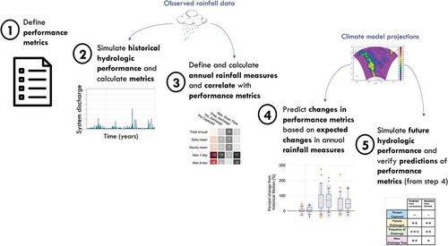
The approach for this analysis consists of five steps, shown in Figure 1. The first step of the analysis defines the performance metrics of interest that could be tracked over time. The second step uses observed rainfall data and continuous hydrologic simulation to estimate the historical hydrologic performance of the site over a 30-year period (1983 to 2014). Performance metrics are then calculated from simulation results. The third step defines and calculates annual rainfall measures (indices) and establishes which of these indices is most indicative of annual performance by calculating correlations with the annual performance metrics. In the fourth step, projections from climate models were used to determine how these rainfall indices are expected to change. Then, based on the expected changes in the rainfall indices (for those determined to the most indicative of the performance metric in step 3), future changes in the performance metrics are predicted. In the final step, projections from the climate models are used for simulation of the bioretention basin under future conditions (2020 to 2060). Future simulation results are then compared to the performance changes predicted based on rainfall indices. Table 1 presents the time periods, dates, and data sources for each of these analyses, and the following sections present more details about each.

Table 1. Analyses carried out in this study and associated time periods

Time period	Dates	Time step	Cities	Data source
Observed	July 2015 to July 2018	5-minute	Pittsburgh	On-site rain gauge and water depth sensors (Civil & Environmental Consultants, Inc and 3 Rivers Wet Weather 2018)
Historical	January 1983 to December 2014	1-hour	All cities in sample	National Centers for Environmental Prediction (NCEP) (NOAA, 2016)
Future	January 2020 to December 2059	1-hour	2 selected cities	4 NA-CORDEX RCM/ESM simulations (Mearns et al., 2017)

Figure 1. Overview of steps used to predict performance of the bioretention basin using annual rainfall measures

2.1. Hydrologic performance metrics

Hydrologic performance of the rain garden was assessed using several annual metrics. The first metric, Runoff Capture Efficiency, also known as the Bioretention Abstraction Volume (Davis et al., 2012) or Reduction from Infiltration (Jennings, 2016), depicts the fraction of runoff water that does not reach the sewer system. This metric is a useful indicator of performance because it describes how much water the rain garden can capture relative to the amount of rainfall received. This is determined as the amount of water that infiltrates through the basin into the ground below as a percentage of total stormwater that enters the site, normalized by the amount of rainfall that was received in that year. Evapotranspiration is not included in this calculation (refer to the Hydrologic model and site section for explanation).

The second metric, Volume of Discharge, also referred to as Overflow Volume (Hathaway et al., 2014) represents the total amount of stormwater that was discharged from the rain garden to the sewer system each year, either due to discharge from under drain pipes or from excess surface runoff that drains into the surface drain and is then discharged to the sewer. Since both mechanisms could cause discharge (overflow) to the sewer, they are not considered separately in the modeling or in this manuscript. This metric is especially useful for tracking the amount of runoff that is discharged to combined sewers; additional stormwater entering the combined system could lead to combined sewer overflows downstream of the rain garden. Reducing on-site discharge could decrease the amount of total overflows to the river.

Similarly, the third metric, Frequency of Discharge, represents the number of times per year that stormwater was discharged to the sewer system. This metric is also of interest to stakeholders within combined sewer service areas since they may be limited to an allowed frequency of combined sewer overflows (CSOs) per year. For instance, communities in Washington State are required to reduce CSOs to an average of one per year, per outfall (Washington State Legislature, 2000). Tracking the frequency of discharge from rain gardens over time could help municipalities to minimize upstream discharges in order to meet strict requirements like these. Frequency of Discharge is calculated by counting the number of times that there was flow present in the outfall pipe from the system to the sewer.

The fourth and final metric is the Maximum Surface Detention Time, which calculates the maximum length of time that water is stored on the surface of the bioretention basin. Stormwater regulations in Pennsylvania and elsewhere require basins to drain fully in less than 48 h (PA DEP, 2006), so this metric is used to assess how well these basins are meeting this requirement. Although back-to-back rainfall events have been shown not to be a concern (Wadzuk et al., 2017), other authors have used this metric to determine risk of mosquito breeding in standing surface water, which may pose a threat in certain regions (Jennings et al., 2015; Sell et al., 2009). Surface Detention Time is calculated as the length of continuous time that the depth of water on the surface is greater than 0. The basin is considered “drained’’ if water is not present for 30 min or longer. The metric can be used to assess the number of times per year that water ponds on the surface for longer than a specific time period (e.g., 48 h) or, if the threshold is not exceeded, how close it comes to this level and at what frequency.

2.2. Hydrologic model and site

2.2.1. Example site

The example site used for the simulation is located in Pittsburgh, Pennsylvania (40.46, −79.92) within the Allegheny River Basin. The site was selected because it has characteristics typical of bioretention basins, including a vegetated surface layer that allows for ponding, a subsurface soil layer that promotes infiltration, a gravel layer that provides additional subsurface storage and encourages infiltration, and an underdrain to control releases to the sewer system (Davis et al., 2009; Jennings, 2016; PA DEP, 2006).

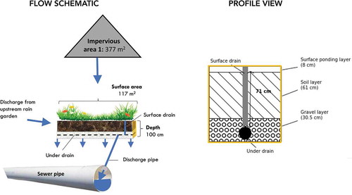
Figure 2 presents a schematic of the site and a profile view of the storage layers of the bioretention basin. Runoff that enters the rain garden from impervious areas or from an upstream rain garden is infiltrated and stored in a 61 cm deep engineered soil layer (71 m³ of storage), where it is available for uptake by the plants. Water then enters a 30.5 cm deep gravel layer (36 m³ of storage), which consists of 10 cm (4 in) of protective chinking stone and 20.5 cm (8 in) of crushed stone. This layer sits atop a ~ 150 mm perforated underdrain that is controlled with a weir and an orifice. When inflow exceeds infiltration, water can pond on the surface to a depth of 7.6 cm (3 in). Underdrain and surface flows from the rain garden are routed to a solid PVC pipe that discharges to the combined sewer system. Post-construction soil samples report the soil as 86 – 88% sand, 10% silt, and 2 – 4% clay (A&L Great Lakes Laboratories, Inc, 2015). More details about the site are presented in Section 2.1 of the Appendix.

Figure 2. Flow schematic of site and model (not to scale), left, and profile view of the bio-retention layers, right. The impervious areas drain to the surface of each garden. Rain garden 1 can drain to rain garden 2 through surface runoff or under drain flow

2.2.2. Continuous hydrologic simulation

The PC Stormwater Management Model (PCSWMM) Version 7.1 (Computational Hydraulics Int, 2018) was used to model the site using continuous hydrologic simulation, which characterizes system response over time and accounts for antecedent soil moisture conditions for consecutive storm events. PCSWMM was also selected for its ability to model multi-layer bioretention systems. Evapotranspiration was not considered in the model because prior studies have found that runoff reductions from evapotranspiration (ET) are negligible (Jennings, 2016; Jennings et al., 2015). Jennings (2016) found that across 35 locations in the U.S. evapotranspiration from bioretention basins contributed only 0.16% to 1.06% of runoff reduction. Brown and Hunt (2010) reached a similar conclusion when the found ET to only account for 3% to 5% of stormwater attenuation in a bioretention cell. The contribution from ET is small because the process takes place only during daytime dry weather. The very small contribution from ET is within the bounds of uncertainty of the performance of the RG and thus excluded from the modeling presented here.

In the model, runoff enters the rain garden from four sources: two roof areas, one pavement area, and one upstream rain garden (see Figure 2). Both rain gardens are modeled as bioretention cells with a soil layer, gravel layer, and an underdrain. Although the project site contains two rain gardens, and both were modeled, in order to limit the scope and ease comprehension of results, only the downstream rain garden that has the potential to drain to the sewer was evaluated for performance. Table A3 in the Appendix presents the sub-basin areas and cumulative runoff volumes.

Subcatchment and conduit parameter values were estimated using a combination of as-built drawings (CH2MHILL, and Viridian Landscape Studio, 2011), literature sources, and model default values. Surface, soil, storage, and underdrain parameters specific to the bio-retention cells were based on typical ranges for bio-retention cell parameters provided in the SWMM Reference Manual (Rossman & Huber, 2016). Specific values within these ranges were initially estimated based on pre-existing field sampling (A&L Great Lakes Laboratories, Inc, 2015), as-built drawings (CH2MHILL, and Viridian Landscape Studio, 2011), and when no information was available, mid-point values of the range or model default values. Parameter values were adjusted within a reasonable range so that simulated annual performance metrics for Pittsburgh were fairly aligned with observed performance values calculated using on-site data collected in Pittsburgh. Table 2 presents a subset of the model parameters for the bioretention basin of interest. Additional parameter values and information relating to their selection are reported in Section 2.2 of the Appendix, along with more information about the on-site data collected in Pittsburgh.

Table 2. Selected parameters of the bioretention basin (downstream) from the SWMM model

Parameter (units)	Value	Estimation method/source
Surface berm height (in)	3	As-built drawings (CH2MHILL, and Viridian Landscape Studio, 2011)
Surface slope (%)	0.01	As-built drawings (CH2MHILL, and Viridian Landscape Studio, 2011)
Soil thickness (in)	24	As-built drawings (CH2MHILL, and Viridian Landscape Studio, 2011)
Soil porosity (volume fraction)	0.36	Soil sampling (A&L Great Lakes Laboratories, Inc, 2015); Adjustment to reflect observed performance
Soil conductivity (in/hr)	2.0	SWMM Reference Manual range (Rossman & Huber, 2016); Adjustment to reflect observed performance
Storage layer thickness (in)	12	As-built drawings (CH2MHILL, and Viridian Landscape Studio, 2011)
Storage layer seepage rate (in/hr)	2.5	As-built drawings (CH2MHILL, and Viridian Landscape Studio, 2011); Adjustment to reflect observed performance

2.3. Historical performance of the rain garden

2.3.1. Historical precipitation data

Although the example site is located in Pittsburgh, this configuration could be present in other locations. Rain garden performance has been shown to be dependent on rainfall patterns (e.g., duration and frequency of storms) (Jennings, 2016), thus several different locations were evaluated. Bukovsky climate regions (Bukovsky, 2011), which are smaller and more hydrologically similar than NOAA climate regions (Bukovsky et al., 2019), were used to identify cities that were representative of the various U.S. climate zones. One city per Bukovsky climate region was selected for a total of 17 U.S. cities: Amarillo, TX; Boise, ID; Boston, MA; Boulder, CO; Charlotte, NC; Chicago, IL; El Paso, TX; Fargo, ND; Memphis, TN; Missoula, MT; New Orleans, LA; Phoenix, AZ; Pittsburgh, PA; Portland, OR; St. Louis, MS; San Antonio, TX; and San José, CA. Hourly observed precipitation data for the period from 1983 to 2014 were obtained from the NOAA National Center for Environmental Information (NOAA, 2016) for the weather station located closest to the city. Exact coordinates are provided in Table A1 in the Appendix.

2.3.2. Historical simulation and performance metrics

The historical rainfall data from the period 1983 to 2014 were used to evaluate the hypothetical historical performance of the rain garden system. The hourly historical simulation results were then used to calculate the annual performance metrics in each city. Annual percent capture was calculated as the total stormwater infiltrated below the RG divided by the sum of flows entering the RG each year. Volume of discharge was calculated as the annual sum of hourly volumes from the outflow pipe, which were converted from hourly flow rates. Frequency of discharge was calculated by counting the number of hours where the outflow pipe contained flow. Maximum surface drainage time was calculated as the maximum amount of consecutive time each year where the depth on the surface of the RG was above 0.1 mm.

2.4. Rainfall indices most indicative of annual performance

2.4.1. Rainfall index definition

To determine which rainfall indices could most affect rain garden performance and, therefore, be suitable surrogates for performance monitoring, an extensive list of annual precipitation indices was defined. The list was developed from the literature (e.g., Chen et al., 2015; Karl & Knight, 1998) and through recommendations from the Expert Team on Climate Change Detection Monitoring and Indices (Karl et al., 1999; Peterson et al., 2001). Each index, listed in Table 3, was calculated based on hourly and daily rainfall amounts using the same observed rainfall data that were used in the historical simulation. Indices were grouped by the aspect of precipitation they describe: the central tendency of rainfall, magnitude, proportion, or frequency of extremes, or frequency of wet and dry days. The ‘set’ column represents the different variations of each index that were tested. Each index was calculated for each year of historical rainfall data (30 data points for each index).

Table 3. Rainfall indices evaluated in this study. The ‘set’ column represents the different variations of each index that were tested

Index	Set	Description	Implication	Indicator
total	n/a	Total annual precipitation (mm)	Wet or dry year	Central tendency
nintd	nε (µ, q50)	Mean or median daily intensity of rain days (mm)	Intensity of rain days
ninthr	nε(µ, q50)	Mean or median hourlyintensity of rain hours (mm)	Intensity of rain hours
maxnd	nε (1,2,3) days	Greatest n-day totalprecipitation (mm)	Measure of extremeswith duration less thanor equal to drainagerequirement	Extreme magnitude
qpd	pε (90,95,99) quantile	pth percentile of rain dayamounts (mm/day)	Intermediate to raredaily extremes
qph	pε (90,95,99) quantile	pth percentile of rain houramounts (mm/hr)	Intermediate to rarehourly extremes
totqp	pε (90,95,99) quantile	Total rain from daily qthpercentile or greater (mm)	Total from intermediateto rare extremes	Extreme total
propqp	pε (90,95,99) quantile	Proportion of total annualrainfall above qth percentile (%)	Measure of extremescompared to total received	Extreme proportion
excdn	nε (10,25,50) mm	Number of rain days withprecipitation ≥ n mm (days)	Intermediate to raredaily extreme events	Extreme frequency
raind	n/a	Number of rain days whereprecipitation > 0.1 mm (days)	Daily precipitationoccurrence	Frequencywet & dry
ncwd	nε (µ, max)	Mean or max number ofconsecutive wet days whereprecipitation > 0.1 mm (days)	Measure of average tolong-duration storms
ncwh	nε (µ, max)	Mean or max number ofconsecutive wet hours whereprecipitation > 0.01 mm (hours)	Measure of average tolong-duration storms
ncdd	nε (µ, max)	Mean or max number ofconsecutive dry days whereprecipitation < 0.1 mm (days)	Measure of risk ofdryness and antecedentsoil conditions

2.4.2. Correlation of rainfall indices and performance metrics

The correlation of the rainfall indices to the annual performance metrics was used to determine which indices are most indicative of annual performance. Correlation was tested using the Pearson correlation coefficient, which measures the linear relationship between two data sets that are normally distributed. The rainfall indices and performance metrics were verified to be normally distributed using an omnibus test of normality based on D’Agostino and Pearson (1973) test combining skew and kurtosis. The null hypothesis could not be rejected with a p-value of 0.001 for all variables.

Correlations were quantified as negative (representing an inverse relationship) or positive, and ranging from low (0 to 0.34), moderate (0.35 to 0.64), high (0.65 or above), and very high (0.9 or above). Indices that have high or very high correlations to the performance metrics were selected as the indices most indicative of performance. If several rainfall indices were highly correlated with the same performance metric, it is possible that these indices are also correlated with each other. Thus, correlations between indices were also evaluated. If a given pair of indices was determined to be correlated, only one was considered further. The selection of rainfall indices most indicative of performance for individual cities is discussed in the results section.

2.5. Expected changes in future rainfall and performance metrics

2.5.1. Source of climate model output

This study used output from regional climate models (RCMs) from the NA-CORDEX project (Mearns et al., 2017) to evaluate anticipated future changes in rainfall. The RCMs in the NA-CORDEX are simulated using Earth System Models (ESMs) as inputs (Heavens et al., 2013) over the continuous period from 1950–2099. This study used the four RCM-ESM combinations (see Table A2 in the Appendix) available at a 1-h time step and simulated at the 50-km resolution with the RCP 8.5 emissions pathway, which is the scenario with the highest assumed greenhouse gas emissions (Riahi et al., 2011). The 1-h time step from RCMs is crucial for continuous hydrologic simulation models to capture localized rainfall-runoff interactions (Cook et al., 2017; Durrans et al., 1999) and the 50-km resolution was chosen over the 25-km resolution because future rainfall intensities were greater and provide a higher level of protection (Cook, 2018). More details are provided in Appendix Section 1.2.1.

Although four RCM-ESM projections were analyzed, only two are discussed: CanRCM4/CanESM2 (CANCAN) and RegCM4/MPI-ESM-LR (MPIREG). They provide a complementary representation of the uncertainty range that could be expected in the future. The CANCAN model generally predicts a wetter and more variable future, while the MPIREG model predicts drier and less variable future. The CANCAN model will be referred to as the wetter future, while the MPIREG model will be referred to as the drier future.

2.5.2. Bias-correction of climate model output

The raw RCM-ESM combinations are an areal average of precipitation across a 50-km grid cell, which are not representative of rainfall values at a weather station (Gregersen et al., 2013). This analysis uses a bias-correction method, called Kernel Density Distribution Mapping (KDDM), to adjust the RCM-ESM simulations to the station scale (McGinnis et al., 2015). Hourly observed data from the NCEI (NOAA, 2016) for the stations reported in Table A1 in the Appendix for the period 1950 to 2010 were used to find a non-parametric relationship with the raw climate model output for a historical time period (1950–2010). This relationship was used to adjust the entire gridded climate model time series (1950–2099) to the station scale. More details are provided in the Appendix Section 1.2.2. A major benefit to the KDDM method is that the timing of rainfall events simulated from the RCMs are maintained in the bias-corrected data, which allows the performance analysis to incorporate changes in the frequency of storm arrival as well as changes in rainfall intensity.

2.5.3. Predicting future changes in performance metrics from rainfall projections

To estimate changes in the future, rainfall indices were calculated for each year of the bias-corrected climate projections. The percent change of each index was calculated for each year with respect to the median of the historical rainfall indices over the 30-year period (1983–2014). In order to evaluate if rainfall indices can be used as a proxy for on-site performance data, the change in the rainfall index most indicative of each performance metric was used to predict how that performance metric would change in the future. For instance, if the maximum 1-day rainfall value was most indicative of maximum surface drainage time, and the maximum 1-day rainfall was expected to increase by 25-50% based on the climate projections, then the maximum surface drainage time would be predicted to increase by a similar magnitude in the future (assuming there was a positive correlation between these variables).

2.6. Simulating future performance

The predicted changes in performance metrics (based on correlations to rainfall indices) were then compared to the simulated results for the future time period to determine if the predictions were correct. Using the calibrated hydrologic simulation model, future performance of the RG was simulated for two out of 17 cities using the bias-corrected climate model projections at the 1-hourly timestep as inputs. Annual performance metrics were calculated from the future simulation results for each city and climate model projection in the same manner as the historical simulation. Changes in the performance metrics with respect to the historical period were compared to predicted changes in performance based on the rainfall projections.

3. Results and discussion

3.1. Simulated historical rain garden performance

In most cities, the example bioretention basin performed well during the historical simulation period. Figure 3 presents the four simulated performance results for all 17 cities over the period from 1983 to 2014 along with the rainfall indices that were strongly correlated to that metric in many cities (discussed in the following section). The average total annual rainfall in each city is also shown in the figure, represented as the size of the marker. The cities are ranked based on this value, from lowest to highest across the horizontal axis (Phoenix has the lowest and New Orleans has the highest). Panel (a) shows the first performance metric, the annual percent of runoff captured and the average daily 99th quantile of rainfall for each city, represented by marker color. Panel (b) presents the volume discharged to the sewer and total rainfall from ≥ the 95th quantile (averaged across years) as the color. Panel (c) presents the frequency of discharge to the sewer and total rainfall from ≥ the 90th quantile (averaged across years) as the color. Panel (d) shows the maximum number of hours to drain the surface and maximum 1-day rainfall (averaged across years) as the color. The median annual value of the performance metric is represented by the marker location on the vertical axis, and the range shows the minimum and maximum annual value during the historical period.

Figure 3. Annual rain garden performance over historical period [1983–2014] for 17 cities, including: (a) percent of runoff captured annually, (b) the volume of discharge to the sewer, (c) the frequency of these discharges, and (d) the maximum number of hours to drain the surface. The marker represents the median value across all years, the size of the marker represents the average total annual rainfall in that city, and the color of the marker represents an average annual rainfall index (listed in color bar legend). The cities are ranked based on their average total annual rainfall, from lowest to highest across the x-axis

Results show that for more than half of the historical period, the simulated system captured at least 90% of rainfall (Figure 3(a)), overflowed fewer than 10 times (Figure 3(c)), and had a maximum drainage time of fewer than 4 h (Figure 3(d)) in all but two cities. These historical performance values are excellent, but not surprising given the large capacity for storage of the rain garden. Capture efficiency is within the bounds reported by Jennings (2016) who evaluated simulated rain garden performance in 35 locations within the contiguous U.S.

These historical simulation values can be used to set thresholds for evaluating performance degradation over time, as well as for scheduling maintenance. If the basin performs well when evaluated across the historical rainfall conditions, stakeholders may want to undertake adaptation or maintenance actions when percent capture (or another metric) falls below a threshold that is considered unsatisfactory, for example, 80% volumetric capture per year. However, if the basin is already performing near or below this 80% value based on the historical evaluation, then stakeholders may want to accept a lower threshold, or consider expanding the basin.

These findings suggest that cities with lower total annual rainfall tend to perform better because there is less rainfall overall that needs to be captured. However, total annual rainfall is not the only indicator of performance. The magnitude and total quantity of extreme rainfall are also important indicators of how well a rain garden will perform in a city. As expected from the correlation analysis, cities with the highest daily 99th quantile rainfall (e.g., in Figure 3(a), San Antonio and New Orleans) captured the least amount of runoff. Cities with the highest total rainfall from extremes discharged the most stormwater with the highest frequency (e.g., in Figure 3(b,c), Memphis and New Orleans). Finally, cities with high maximum 1-day rainfall (Figure 3(d)) values had the longest surface drainage times.

3.2. Strong relationships between rainfall indices and performance metrics

The relationships between rainfall indices and performance metrics were confirmed by evaluating the strength of their correlations. During the historical period, strong correlations exist between the performance metrics and several rainfall indices in many cities. Figure 4 shows the number of cities (out of 17) where a strong correlation (>0.64) exists between the rainfall index and performance metric as a heat map. The rainfall indices that have the highest number of strong correlations for each performance metric are outlined in dark blue. The total number of cities where strong correlations were found between performance metrics and rainfall indices are shown in the last row of the figure.

Figure 4. Number of cities (out of 17) where a strong correlation exists between rainfall indices (rows) and rain garden performance metrics (columns) in the historical period [1983–2014]. The rainfall indices that have the highest number of strong correlations for each performance metric are outlined in blue

In more than half of cities, strong correlations exist between the performance metrics and at least one rainfall index. However, some cities have very few or no strong correlations between rainfall indices and performance metrics, including Portland, Missoula, San José, Boston, and Boise. The rain garden performed very well in these cities, with zero, or nearly zero, discharge in almost every year. In these cases, it does not rain enough to result in a discharge, and thus, there are not enough data to establish strong correlations between performance metrics and rainfall indices.

In cities where strong correlations do exist, the performance metrics tend to be strongly correlated to rainfall indices related to the magnitude or total quantity of extreme rainfall. For instance, the percent captured and the maximum drainage time are strongly correlated to the maximum 1-day rainfall in the largest number of cities, meaning that the magnitude of maximum daily rainfall that occurs in a year can provide an indication of how much rainfall was captured or how long the surface took to drain. Similarly, the total amount of rainfall from extremes (e.g., the quantity of rain received that is greater than the 90th quantile storm) can be used to understand how much and how often runoff was discharged from the system. This analysis confirms that when adequate data are available, strong relationships can be established between performance metrics and rainfall indices, and as a result, tracking rainfall indices can be used to evaluate rain garden performance.

3.3. Rainfall indices most related to performance during historical simulation

In order for rainfall indices to be used as a proxy for performance, a specific rainfall index should be selected as representative of the performance metric of interest to the stakeholder. If multiple performance metrics are of interest to the stakeholder, then multiple rainfall indices may be tracked as a proxy for each metric. However, the index used to represent a performance metric may not be the same as the general trends observed across all the cities (and described in the previous section). Selecting a rainfall index as representative of a performance metric requires location-specific analysis because the indices with strong correlations to individual performance metrics vary depending on the city. Figure 5 highlights this fact by showing correlations between performance metrics and rainfall indices for two specific cities, Pittsburgh and Memphis, which were selected because they have higher amounts of rainfall than many cities in the western U.S. and are thus more likely to employ green infrastructure to reduce stormwater runoff. Taking the example of frequency of discharge, the indices with strong correlation to this metric are indeed different in each city, and different from the results across all cities, discussed previous section. In Pittsburgh, the frequency of discharge is most highly correlated to the magnitude and frequency of extreme rainfall, while in Memphis, it is more strongly related to the total rainfall. These correlations vary depending on the city because rainfall patterns vary in frequency, magnitude, and total quantity in each city, and the rain garden system will respond differently to these differences.

Figure 5. Correlations between rainfall indices and all performance metrics in Pittsburgh (left) and Memphis (right) for historical period [1983–2014]. Grey colors represent positive correlations, while reds represent negative correlations

Figure 5 also shows that for a specific city, several rainfall indices can be strongly correlated to the same performance metric. For instance, the volume of discharge in Memphis is strongly correlated to the total from ≥90th quantile, and the number of rain days >50 mm. Many of these indices are also strongly correlated with each other (refer to Section 3.1 in the Appendix), and it is not immediately clear which one of these indices should be selected as most indicative of the performance metric. Multiple indices could be tracked, but need not be if they are related to each other.

To select the index most indicative of a specific performance metric, analysts may want to choose the rainfall index that is easiest to calculate, like the maximum 1-day rainfall, or that is easily understood by stakeholders, like the number of rain days above 25 mm. Alternatively, it may be important to ensure that the strength of correlations are robust against a margin of uncertainty for parameter estimation. In this case, a sensitivity analysis could be conducted to determine which correlations remain strong when model parameters are altered. Similarly, model parameters could be modified to represent potential changes in site conditions that are unrelated to rainfall, like soil conductivity. The indices with correlations most robust against changes would be selected. Finally, an alternative approach is to select the index with the highest absolute correlation, even if the correlation is only marginally higher than other indices.

In this analysis, the last approach was used to select the indices most indicative of the four performance metrics in both cities. If two or more indices had the same correlation to a performance metrics, then the index that was easiest to interpret was selected. For instance, in Memphis, the total annual rainfall and the total from ≥ the 90th quantile both have a strong correlation of 0.71 to the frequency of discharge. The total annual rainfall was selected as most indicative of frequency of discharge because the meaning is more intuitive than the other index. The indices selected as most indicative of each performance metric in each city are summarized in Figure 6.

Figure 6. Rainfall indices most indicative of performance for historical period [1983-2014]. The colors for each performance metric correspond to the rainfall indices presented in Figure 7

Figure 7. Percent change in rainfall indices for two climate model simulations, drier future (orange) and wetter future (purple) in Pittsburgh (top) and Memphis (bottom). The box and whisker plots represent the range of the percent change for each year and each climate model for the future period [2020–2059], with respect to the historical period [1983–2014]. The middle line of the box plot represents the median over the 40-year future period; the box outline shows the 25th and 75th quantiles, and the whiskers show the 5th and 95th quantiles. Outliers are shown as orange dots (for the drier future) and purple stars (wetter future). The grey shading represents the historical range (in terms of percent change from the median). The black dashed line at zero represents no future change. The indices highlighted with color are those that were selected as most indicative of each performance metric, including capture efficiency (blue), volume discharged (yellow), frequency of discharge (green), and maximum drainage time (pink)

3.4. Expected changes in rainfall and predicted changes in performance metrics

Each rainfall index in Figure 6 has a relatively high correlation to the related performance metric, which means that if the rainfall index changes, the performance metric is expected to change in a similar manner. This section presents projected changes in precipitation in the future for the selected rainfall indices, and then discusses how performance would be predicted to change, based on these projections.

Figure 7 presents the percent change of each rainfall index for the two selected climate model projections (drier and wetter future) for Pittsburgh and Memphis. The box and whisker plots represent the range of the percent change across all future years (2020 to 2059). The colored line shows the median over the future period, the box outline shows the 25th and 75th quantiles, and the whiskers show the 5th and 95th quantiles. Outliers are shown as orange dots (drier future) and purple stars (wetter future). The grey box represents the historical range (in terms of percent change from the median). The indices highlighted with color are those that were selected as most indicative of each performance metric in the previous section (see Figure 6). Blue highlight refers to the capture efficiency, yellow to the volume discharged, green to the frequency of discharge, and pink to the maximum drainage time.

In Pittsburgh, both climate model scenarios project similar changes: increases in extreme rainfall (e.g., maximum 1-day rainfall) and in the average number of consecutive dry days (index to the far right of the graph). This results in total annual rainfall remaining similar to the past. The drier future (orange) generally predicts smaller increases in extremes and less variability than the wetter future (purple). The index most indicative of the runoff capture efficiency, proportion of rainfall from the 90th quantile or greater, is expected to increase (median value), and climate projections suggests that the proportion of extremes will surpass the historical upper bound in 50-75% of future years. As a result, capture efficiency is expected to decrease in the wetter and drier climate scenarios, with several years below the historical lower bound. The average hourly intensity, most indicative of volume of discharge and maximum drainage time in Pittsburgh, is predicted to increase (median value) in the wetter scenario, but still remain within the historical range. Based on projected increases in number of days where rainfall >25 mm, frequency of discharge is expected to increase in both climate scenarios, with fewer than 25% of years outside of the historical range. Finally, the total rainfall from the 99th quantile or greater, most indicative of maximum drainage time, is predicted to increase (median value), with fewer than 50% of years falling outside the historical range.

In Memphis, the two climate model simulations predict opposing trends. The wetter future predicts that Memphis will have considerably more total rainfall, due to higher intensities, while the drier future predicts Memphis will have about the same median total, due in part to long dry spells and some years with more variability. The rain garden is thus predicted to perform much worse in the wetter scenario, and sometimes better in the drier future scenario. Based on changes in the daily 95th quantile, capture efficiency in Memphis would be expected to decrease in both scenarios, with 50% to 75% of future years capturing less runoff than was observed in the historical period. Changes in number of days where rainfall >50 mm in both future scenarios indicate that median volume of discharge would be expected to decline, including some years with higher volumes discharged than in the past.

Based on changes in the total annual rainfall in the drier future, increases in the frequency of discharge are predicted, with less than 25% of future years having more discharge events than in the historical period. In the wetter scenario, the median total annual rainfall remains about the same, but some years are expected to have more discharge events than in the past, and some years fewer events because variability increases. Finally, since the maximum 5-day rainfall increases in both scenarios (median), maximum drainage time would increase overall. This increase is larger in the drier future, with about 50% of years expected to have longer drainage times than in the past. In the wetter future, about 25% of years are expected to have drainage times higher than in the historical period.

The predictions for each performance metric are summarized in Figure 8 for both climate model projections (drier and wetter future) and cities (Pittsburgh and Memphis). The predicted values were estimated using the corresponding rainfall indices shown in Figure 7. Plus signs (+) signify that an increase in the median performance metric was predicted, based on the projected change in the rainfall index associated with the performance metric. Minus signs (-) signify that a decrease in the median performance metric was predicted, based on the associated rainfall index. The number of plus signs refer to the predicted magnitude of change (less than 25%, between 25% and 75%, or greater than 75%). The arrows signify that some of the future years were predicted to fall outside the upper (↑) or lower (↓) historical bounds. The number of arrows conveys the percentage of future years that were predicted to be outside the historical range: less than 25% (one arrow), between 25% and 50% (two arrows), and more than 50% of years (three arrows). An X implies that none of the future years were predicted to lie outside the historical range. For all performance metrics except percent capture, the direction of change is equal to the direction of change of the rainfall index. However, percent capture is inversely correlated with the associated rainfall indices, thus an increase in the associate rainfall index leads to a predicted decrease in the percent capture (or vice versa). The predicted changes in performance metrics are compared to the change in performance metrics calculated using the hydrologic simulation model and future bias-correction climate model projections.

Figure 8. Predicted and simulated changes in performance metrics in the future [2020–2059] for both cities (Pittsburgh and Memphis) and both climate model scenarios (drier and wetter future) with respect to the historical period [1983–2014]. Predicted changes are based on projected changes in rainfall indices most indicative of each performance metric and simulated changes are calculated from the SWMM model simulations using climate projections. For all performance metrics except percent capture, the direction of change is equal to the direction predicted by the rainfall index. However, percent capture is inversely correlated with the associated rainfall indices, thus an increase in the associate rainfall index leads to a predicted decrease in the percent capture

3.5. Simulated future rain garden performance

The previous section identified trends in the rainfall indices most indicative of the performance metrics, and provided a hypothesis for how the rain garden would perform based on these trends (see Figure 8). This section presents the simulated performance of the rain garden in the future and identifies whether simulated performance shows patterns consistent with the predictions. Figure 9 presents the simulated performance of the rain garden in the two future scenarios (shown in orange and purple), and in the historical period, for reference (shown in black). The y-axis shows the cumulative probability (%) and the x-axis shows the magnitude of each performance metric in percent, volume (L/yr), number, and hours for the four metrics, respectively. The median value for each scenario is highlighted with a vertical, dashed line, while historical range is represented by vertical, grey shading. These results are also summarized in Figure 8 as magnitude of simulated change (less than 25%, between 25% and 75%, or greater than 75%) and the percentage of future years that were simulated to be outside the historical range (less than 25%, between 25% and 50%, and more than 50% of years).

Figure 9. CDFs of four performance metrics (as rows), (a) percent of runoff captured, (b) volume of discharge, (c) frequency of discharge, and (d) maximum hours to drain the surface for all simulations, historical [1983–2014] (black), drier future [2020–2059] (orange), and wetter future [2020–2059] (purple), for Pittsburgh (left) and Memphis (right). The dotted lines cross the x-axis at the median value. The grey shading shows the historical range

Overall, the simulated future performance follows the trends from the rainfall indices; however, predicted and simulated results sometimes vary in the magnitude of predicted change and the number of years expected to fall outside the historical range. In Pittsburgh, the median capture efficiency decreases significantly (p = 0.001) in both climate futures, as predicted, and the median capture efficiency declines as predicted (by less than 25%). However, the simulated range was smaller than predicted by the rainfall indices, meaning fewer years fell outside the historical bounds. In the future simulations, about 30% (wetter future) and 20% (drier future) of future years surpassed the historical bound for capture efficiency in Pittsburgh.

In Pittsburgh, median volume discharged increases significantly (p = 0.001), by a larger amount that was predicted in both future scenarios (between 25% and 75%, not less than 25%). More years were hydrologically simulated to be outside the historical range than predicted based on the rainfall index. Frequency of discharge is modeled to increase by exactly 25% in both future scenarios, from a median of 3 to 4 per year, which is within the predicted range from the rainfall index. Maximum surface drainage time increases significantly (p = 0.001) from 2 to more than 3 h in both futures, using hydrologic simulation. These simulated results are consistent with the predictions using the rainfall indices, except for in the drier scenario. The drainage time was predicted to fall within the historical range for all years; however, hydrologic simulation results show 5% to 10% of years exceeding historical bounds. In general, for Pittsburgh, hydrologically simulated changes match predicted changes from rainfall projections, but the range varies, especially for percent captured and volume discharged. This may be because these two metrics had the weakest correlations out of the four metrics considered.

In Memphis, the hydrologically simulated and predicted performance values are less consistent than in Pittsburgh. In both future scenarios, the hydrologically simulated results show the rain garden performing better than predicted using rainfall indices by capturing more rainfall and discharging less runoff. The frequency of discharge increased as predicted in the wetter scenario, but in the drier scenario, the number of events decrease, rather than increase (by less than 25%). This is the only case where the median performance metric was predicted to increase and instead it decreases in the simulation results. In a few cases, performance was predicted to be more variable than the simulated results show. For instance, some years were predicted to have more discharge events that in the past, and others fewer; however, simulated results show only a few years with fewer discharge events, and none with more. In general, for Memphis, predicted values both overestimate and underestimate the hydrologically simulated range, however, differences are usually within a margin of 25%.

Predictions for Pittsburgh more closely matched the hydrologic simulations than predictions for Memphis. However, this is not necessarily a result of the strength of the correlations in each location. In some cases, the correlation was weaker in Pittsburgh (e.g., for percent capture); however, the median predictions in Pittsburgh still better match the simulated results. The difference in the predictive ability between the two cities is likely a result of the rain garden properties and rainfall patterns in each city. Extreme rainfall is expected to get more intense in Memphis than in Pittsburgh, which would lead to predictions of lower performance. However, given the large capacity of the rain garden, and timing of storms, performance was higher than expected.

4. Conclusions and future work

In this study, annual measures, or indices, of rainfall were evaluated as indicators of hydrologic performance of green infrastructure systems over time. Historical performance metrics were strongly correlated with rainfall indices linked to the magnitude and total quantity of extreme rainfall in a year, and findings suggest that tracking these rainfall indices can provide insight into the future performance of green infrastructure, without the use of hydrologic simulation or on-site sensors. The specific rainfall index used to track performance varies by city because the strength of correlations changes depending on the rainfall patterns in each city. The accuracy of performance predictions was evaluated in two specific cities, Pittsburgh and Memphis, and findings show that the rainfall indices were able to predict the direction of change and the magnitude of change within 25% to 50% in most cases. In some cases, the magnitude of change varied from simulated results, and so did the number of years expected to fall outside the historical range.

The accuracy of predictions was not consistently related to the strength of the correlations between the rainfall index and performance metric, which suggests that there are other factors, such as the design characteristics of the green infrastructure, which would need to be considered to improve the prediction accuracy. It may be possible to apply a regional correction factor to the magnitude of change predicted by the rainfall index in order to determine the magnitude of change in performance. However, regression or more advanced machine learning models that take into account design characteristics may be needed to increase the accuracy of performance predictions from annual rainfall measures.

Developing regional equations of performance for green infrastructure systems as a function of annual rainfall measures would allow GSI performance to be tracked by stakeholders without sophisticated climate models, hydrologic simulations, or on-site sensors. This study demonstrated the promise of this approach; however, additional work is needed to identify the type of changes in rainfall or performance that should result in adaptation or redesign of GSI systems. Due to the variability of rainfall patterns, any one year surpassing a threshold may not be indicative of future trends. Defining acceptable performance thresholds, while not the focus of this study, is an important area that merits further attention.

Acknowledgments

The authors acknowledge data and helpful discussions from those involved in the funding, design and operation of the rain garden system located at the East Liberty Presbyterian Church in Pittsburgh, including: John Buck, Andrew Potts, Dominic Petrazio, and Beth Dutton. The authors would like to thank Felipe Hernandez for assistance using EPA SWMM. Finally, the authors also acknowledge assistance from researchers involved in the NA-CORDEX project, including Linda Mearns, Seth McGinnis, Melissa Bukovsky, and Daniel Korytina.

Disclosure statement

No potential conflict of interest was reported by the authors.

Additional information

Funding

This research was sponsored by the National Science Foundation (NSF) (NSF Collaborative Award Number CMMI 1635638/1635686).

Notes on contributors

Lauren M. Cook

Lauren M. Cook was a PhD student in the Civil & Environmental Engineering Department at Carnegie Mellon University; she is now a post-doctoral fellow at the Swiss Federal Institute of Aquatic Science and Technology (Eawag).

Jeanne M. VanBriesen

Jeanne M. VanBriesen is the Duquesne Light Company Professor of Civil & Environmental Engineering and Engineering & Public Policy at Carnegie Mellon University, where she also serves as the Vice Provost for Faculty.

Constantine Samaras

Constantine Samaras is an Associate Professor of Civil & Environmental Engineering at Carnegie Mellon University, where he is the Director of the Center for Engineering and Resilience for Climate Adaptation.

Appendix

1. Data

1.1. Observed rainfall data from 17 U.S. cities

One city per Bukovsky climate region (Bukovsky, 2012; Bukovsky et al., 2019) was selected, for a total of 17 U.S. cities, including Amarillo, TX; Boise, ID; Boston, MA; Boulder, CO; Charlotte, NC; Chicago, IL; El Paso, TX; Fargo, ND; Memphis, TN; Missoula, MT; New Orleans, LA; Phoenix, AZ; Pittsburgh, PA; Portland, OR; Saint Louis, MS; San Antonio, TX; and San José, CA. Table 1 presents characteristics of the locations where data were obtained.

Table A1. Characteristics of cities used in this study

City	State	Bukovsky climate region	Elevation (m)	Latitude	Longitude
Amarillo	TX	C. Plains	1100	35.2	−101.7
Boise	ID	Great Basin	815	43.6	−116.2
Boston	MA	North Atlantic	4	42.4	−71.0
Boulder	CO	S. Rockies	1654	40.0	−105.3
Charlotte	NC	Mid Atlantic	234	35.2	−80.9
Chicago	IL	Great Lakes	187	41.8	−87.8
El Paso	TX	Mezquital	1201	31.8	−106.4
Fargo	ND	N. Plains	273	46.9	−96.8
Memphis	TN	Deep South	79	35.1	−90.0
Minneapolis	MN	Prairie	254	44.9	−93.2
Missoula	MT	N. Rockies	972	46.9	−114.1
New Orleans	LA	Southeast	6	29.9	−90.1
Phoenix	AZ	Southwest	337	33.4	−112.0
Pittsburgh	PA	Appalachia	367	40.4	−80.0
Portland	OR	Pacific NW	6	45.6	−122.6
St. Louis	MO	Prairie	176	38.8	−90.4
San Antonio	TX	S. Plains	230	29.5	−98.3
San Jose	CA	Pacific SW	29	37.3	−121.9

1.2. Climate model simulations

1.2.1. Source of climate model output

This study uses output from regional climate models (RCM) from the NA-CORDEX project (Mearns et al., 2017) to evaluate anticipated future changes in rainfall. NA-CORDEX is a compilation of standardized regional climate model simulations available at an hourly time step, for two different spatial resolutions (50-km and 25-km), over the continuous time period from 1950 to 2100. These models were chosen over other types of downscaled climate models because of their availability at a 1-h time step (Cook, 2018). A sub-daily time step is crucial for continuous hydrologic simulation models that capture highly variable, localized, and short temporal scales of rainfall-runoff interactions (Cook et al., 2017; Durrans et al., 1999).

The RCMs in the NA-CORDEX project use Earth System Models (ESMs) as inputs. ESMs use more complex relationships than those in older Atmosphere-Ocean Global Circulation Models (AOGCMs) (Heavens et al., 2013). At the time of the present analysis, four RCM-ESM combinations were available at the 1-h timestep (presented in Table A2). This study used all four of these combinations simulated at the 50-km resolution using the RCP 8.5 emissions pathway, which is the scenario with the highest assumed greenhouse gas emissions (Riahi et al., 2011). The 50-km resolution was chosen over the 25-km resolution as a more conservative analysis since the 50-km-based simulations predicted higher rainfall intensities for the maximum annual hourly precipitations (Cook, 2018).

Table A2. Regional climate model simulations from NA-CORDEX used in this study

RCM/ESM Combination	Regional Climate Model (RCM)	Earth System Model (ESM)	Abbreviation
RegCM4/MPI-ESM-LR	RegCM4 RCM	‘Max Planck Institute Earth System Model at base resolution’ (MPI-ESM-LR)	MPIREG
WRF/MPI-ESM-LR	WRF RCM	MPI-ESM-LR	MPIWRF
WRF/GFDL-ESM2M	WRF RCM	Geophysical Fluid Dynamics Laboratory Earth System Model, Modular Ocean Version” (GFDL-ESM2M)	GFDWRF
CanRCM4/CanESM2	CanRCM4 RCM	Second generation Canadian Earth System Model (CanESM2)	CANCAN

RegCM4 was originally developed at the International Centre for Theoretical Physics (ICTP) and simulated for NA-CORDEX at the National Center for Atmospheric Research (NCAR). WRF was developed and simulated at NCAR. CanRCM4 was developed and simulated at the Canadian Centre for Climate Modeling and Analysis.

1.2.2. Bias-Correction of climate model output

The raw RCM/ESM simulations are an areal average of precipitation across a grid cell (50 km x 50 km). These data are not representative of rainfall values at the station (or city) scale, and thus must be adjusted to match the scale of the observed values. The method used in this analysis to adjust the RCM-ESM simulations to the station scale is called Kernel Density Distribution Mapping (KDDM) (McGinnis et al., 2015). Hourly data from the period 1950 to 2010 were used for this bias-correction. Data were obtained from the NOAA National Center for Environmental Information (NOAA, 2016) for the stations reported in Table A1 above.

This method is a type of non-parametric bias-correction that uses a relationship between the observed rainfall time series (1950-2013) and the gridded climate model time series for the historical time period (1950-2013) to adjust the entire gridded climate model time series (1950-2099) to the station scale. The relationship between the observed rainfall time series and the gridded climate model time series is defined by fitting a transfer function between their empirical cumulative probability distribution functions (CDFs). First, empirical probability density functions (PDFs) are computed using kernel density estimation; these PDFs are then integrated using the trapezoid rule to calculate CDFs. Equal points of probability from the CDFs are mapped against each other and the resultant mapping is then fitted with a spline. The equation of this spline is the transfer function between the observed data and the historical climate model simulation output. The function is then applied to the 150-year time series of the climate model simulations to obtain bias-corrected values at the station scale.

After this correction, the statistical distribution of the observations is more consistent with the statistical distribution of the historical period of the bias-corrected data. The major benefit of using the KDDM method to convert an RCM time series to a station scale is that the timing of rainfall events simulated from the regional climate models at the sub-daily level are maintained in the bias-corrected data. This allows for analysis of future rain garden performance not only based on increases in volume or intensity, but also due to changes in the frequency of storm arrival that are portrayed in the climate models.

2. SWMM model and example site

2.1. Example site and model configuration

The site contains two rain gardens that collect water from adjacent roof and pavement areas. The upstream rain garden (RG) collects runoff from an impervious area of 400 m². This RG drains into a downstream rain garden, which also collects runoff from an impervious area of 377 m². The downstream rain garden has the potential to overflow to the combined sewer system and is the one that is evaluated for performance in the study. Runoff that enters either rain garden is infiltrated and stored in a 61 cm deep engineered soil layer where it is available for uptake by the plants. Water then enters a 30.5 cm deep gravel layer, which sits atop a ~150 mm perforated underdrain. When inflow exceeds infiltration, water ponds on the RGs to a depth of 76 mm (3 in), enabled by the elevation difference between the top of the RG and the street. Ponded water can flow into a vertical surface drain that connects to the underdrain. Flow in the underdrain is controlled with a weir and an orifice.

Eight sub-basins are modeled to represent four roof areas, two pavement areas, and two rain gardens. At the site, the outlet of the under drain of the downstream RG flows into a solid HDPE pipe and then into a perforated under drain. In the model, the perforated pipe is modeled as an underdrain (available with the bio-retention feature in the SWMM model). Underdrain and surface flow of the upstream RG is routed to the downstream RG. Underdrain and surface flow from the downstream RG is routed to a solid PVC pipe that discharges to the combined sewer system. The orifices and weirs controlling the underdrain flow are accounted for in the model using storage, orifice, and weir nodes (Rossman, 2015). Table A3 presents the sub-basin characteristics and flow patterns.

Table A3. Drainage area characteristics of SWMM model

Drainage Area	Sq. Ft	Sq. Meters	Slope	% Impervious	% Zero-Impervious	Drains to
Roof 1	1440	134	2%	100	100	Upstream RG
Roof 2	1360	126	2%	100	100	Upstream RG
Pavement 1	1500	139	2%	100	25	Upstream RG
Roof 3	700	65	2%	100	100	Downstream RG
Roof 4	2500	232	2%	100	100	Downstream RG
Pavement 2	860	80	2%	100	25	Downstream RG
Upstream RG	1262	117	0.1%	0	25	Downstream RG
Downstream RG	907	84	0.1%	0	25	Outfall

2.2. SWMM model parameter selection

Model parameter values were first selected using a combination of pre-existing field sampling, as-built drawings, literature sources, model default values, and typical ranges for bio-retention cell parameters provided in the SWMM Reference Manual (Rossman & Huber, 2016). Post-construction soil samples of the downstream RG report the soil as sand, with 86–88% sand, 10% silt, and 2–4% clay; whereas, samples from the upstream RG classify the soil as loamy sand, with 86% sand, 8% silt, and 6% clay (A&L Great Lakes Laboratories, Inc, 2015).

Monitoring data were also available at the rain garden site in Pittsburgh. Certain parameters, marked with an asterisk in Table A5, were adjusted within the ranges provided in the SWMM Reference Manual so that annual performance metrics in Pittsburgh were reasonably aligned with observed performance values. In this way, specific conclusions about the relationship between rainfall indices and performance metrics will be representative of a typical bio-retention basin, as well as typical of real-world conditions.

The site in Pittsburgh was equipped with a rain gauge, soil moisture probes, and a Conductivity, Temperature, Depth (CTD) sensor, placed within a cylindrical screen at a 40-inch (1016-mm) depth, which was used to measure water depth before it was discharged to the sewer. Data have been collected from all sensors on a 5-min interval since July 2015. Figure A1 presents a view of the rain garden site.

Figure A1. View of rain garden site at East Liberty Presbyterian Church in Pittsburgh, PA. The tipping bucket rain gauge is placed behind the sign, and the CTD sensor is below ground, near the brown grate. Image source: John K. Buck, Civil & Environmental Consultants, Inc

The model configuration was simulated over the same time period where observed data were available, from July 2015 to July 2018, using the on-site rainfall data at 5-min intervals. Simulated performance results for this period were compared to observed performance from the on-site water level sensors for the same time period. SWMM model parameters for the bio-retention basins were adjusted until an accuracy of ±15% was achieved. These parameters include soil porosity, soil conductivity, wilting point, suction head, void ratio, and seepage rate. Dimensional parameters like soil and surface thickness were not adjusted because they were assumed to be correct based on information from as-built drawings (CH2MHILL, and Viridian Landscape Studio, 2011).

Before a comparison between simulated and observed results could be made, water level data had to be converted to units of flow (and volume) discharged from RG 1 to the sewer. If the water elevation of the CTD sensor was recorded to be above the 5 cm (2 inch) pipe invert, then the pipe was determined to either be full or partially full, depending on whether the water bed elevation was above the top of the pipe, or not. If the pipe was partially full, the radial arc of the water depth was calculated, in order to determine the wetted perimeter of the pipe where water was flowing. If the pipe was full, the entire cross-sectional area of the pipe (5 cm) was used to calculate flow through the pipe using the velocity of water flowing out of an orifice outlet, given the water head. If the pipe was partially full, the partial area and velocity were used to calculate flow. Equations (A1)(A1) $Q\left[ft/s\right]=A\left[f{t}^2\right]\ast C_v\left[ft/s\right]$(A1) and (A2)(A2) $Q=\pi r^2\sqrt{2gh}\ast 0.61$(A2) summarize the calculation. Volume was calculated from the flow rate by multiplying it by the 5-min time interval.

(A1) $Q\left[ft/s\right]=A\left[f{t}^2\right]\ast C_v\left[ft/s\right]$(A1)

(A2) $Q=\pi r^2\sqrt{2gh}\ast 0.61$(A2)

where A is the cross-sectional area, Cv is the water velocity, r is the pipe radius (1 inch), g is the acceleration due to gravity, h is the water height, and 0.61 is a conversion factor.

Figure A2 presents the on-site precipitation and volume discharged over the observed period.

Figure A2. Summary of data from on-site sensors for precipitation (blue lines on top of figure) and volume discharged (red lines on bottom), which was calculated if water level surpassed the discharge pipe invert elevation

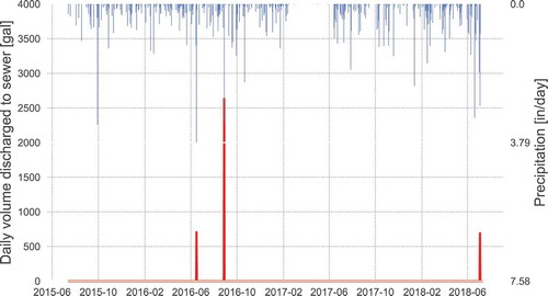
Over the 3-year-observed period, percent capture was calculated to be 98–100% based on water-level sensor data (refer to Table A4 for annual results). SWMM model parameters for the bio-retention basins were adjusted from the SWMM default values until an accuracy of ±15% was achieved for percent of runoff captured. Using simulated results over the calibration period, percent capture was simulated to be 86% to 97%. The annual percent of runoff captured calculated from on-site data and simulation results is presented in Table A4.

Table A4. Annual percent capture during the 4 years in the observed period calculated from observed data from on-site sensors (left column) and calculated from SWMM model simulation (right column) over the period July 2015 to July 2018

Year	Observed on-site	Simulated (observed period)
2015	100%	99%
2016	98%	86%
2017	100%	97%
2018	99%	89%

The bio-retention basins were attributed a surface slope of 0.1%, a vegetative cover of 85%. gravel layer seepage rate of 63.5 mm/hr, and an underdrain discharge rate of 12.7 mm/hr. Soil conductivity and porosity are higher in the upstream rain garden because it has sandier soil. Final parameter values are listed in Table A5.

Table A5. SWMM model parameters. Parameters marked with an asterisk were adjusted to align simulated results with observed performance

Parameters (units)	Upstream RG	Downstream RG	Data Source
Subcatchments  N-Imperv/N-Perv  DStore-Imperv/Perv (in)  Percent Routed  Suction head (in)  Conductivity (in/h)  Initial soil moisture deficit   (fraction)	0.01/0.1 0/0.05 100 2 1 0	0.01/0.1 0/0.05 100 2 1 0	SWMM default SWMM default Site configuration Green Ampt SWMM default SWMM default
Bio-retention cell – surface  Berm height (in)  Vegetation volume (fraction)  Roughness (Manning’s n)  Slope (%)	3 0.8 0.65 0.01	3 0.8 0.65 0.01	As-built drawings As-built drawings/Google Earth (McCuen, 2005; Mustaffa, Ahmad, & Razi, 2016) As-built drawings
Bio-retention cell – soil  Thickness (in)  Porosity (volume fraction)*  Field capacity (volume fraction)  Wilting point (volume fraction)*  Conductivity (in/hr)*  Conductivity slope  Suction head (in)*	24 0.38 0.15 0.09 2.1 8 1.9	24 0.36 0.15 0.09 2 8 1.8	As-built drawings SWMM Reference Manual (Rossman & Huber, 2016) SWMM Reference Manual (Rossman & Huber, 2016) SWMM Reference Manual (Rossman & Huber, 2016) Rawls, Brakensiek, and Miller (1983); SWMM Reference Manual (Rossman & Huber, 2016) SWMM User Manual Rawls, Brakensiek, and Miller (1983); SWMM Reference Manual (Rossman & Huber, 2016)
Bio-retention cell – storage  Thickness (in)  Void ratio (voids/solids)*  Seepage rate (in/hr)*  Clogging factor	12 0.3 2.5 0	12 0.3 2.5 0	As-built drawings SWMM Reference Manual (Rossman & Huber, 2016) SWMM Reference Manual (Rossman & Huber, 2016) Default
Bio-retention cell – underdrain  Drain coefficient (in/hr)  Drain exponent  Drain offset height (in)	0.5 0.5 2	0.5 0.5 2	SWMM User Manual Default As-built drawings
Conduits  Roughness (Manning’s n)  Invert elevation (ft)  Pipe diameter (in)  Orifice diameter (in)  Top of weir elevation (ft)	0.012 904.25 6 2 905.75	0.009 902.25 8 2 903.75	HDPE, PVC (Bishop and Jeppson 1978) As-built drawings As-built drawings As-built drawings As-built drawings

3. Additional Results

3.1. Pairwise correlations between rainfall indices in Pittsburgh

Pairwise correlations between rainfall indices were also examined to understand if these values are related to each other before we consider their role in assessing performance of the rain garden. Figure A3 presents the pairwise correlations between rainfall indices in Pittsburgh as a heat map matrix. Orange colors represent a negative correlation and greys represent a positive correlation. The left and top represent the same metrics in the same order; however, the top rows use abbreviated names (see definitions in Table 3 in the main text).

Figure A3. Heat map of correlations among rainfall indices for Pittsburgh. Darker colors represent a stronger correlation between rainfall indices

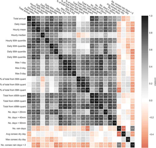
The total annual rainfall is weakly correlated (0.4) with the number of rain days. It is most highly correlated with the 90th quantile (0.7), the number of rain days above 25 mm (0.7), and the maximum 5-day rainfall (0.6). It is very weakly correlated to the average and maximum consecutive rain days (0.1), and the proportion of the total from the 90th quantile or above (0.0).

The proportion of the total rain from the 90th quantile is a promising metric to consider because rain garden performance is potentially related to both the amount of rainfall entering in a given time (total annual) and the quantity of individual, large storms (90th quantile) during that same time period. However, the proportion between these two metrics is not correlated with either of them (−0.01 and 0.12, respectively). The propqp is more closely related to the number of long and extreme storms, with a moderate correlation to the maximum 5-day rainfall and to the number of rain days above 50 mm. This is coherent because if total rainfall and 90th quantile rainfall both increased, then the ratio of q90 to the total may not change, even though the individual values do. Since propqp is nearly independent of these individual metrics, it may provide an indication of performance that neither of these two other metrics can provide individually.

The strongest positive correlations, apart from those between the maximum n-day rainfall values, exist between the total annual precipitation and the 90th quantile (0.7), the 90th quantile and the number of rain days above 25 mm (0.7), and the number of rain days above 50 mm and the maximum 2-day rainfall (0.7). The highest negative correlation is between the number of rain days and the average duration of dry days. The number of days with rainfall above 25 mm has the highest number of strong correlations (apart from maximum n-day rainfall), with total annual rainfall, maximum 5-day rainfall, and the 90th quantile of daily rainfall. The number of days with rainfall above 25 mm has the highest number of strong correlations: to total annual rainfall, maximum 5-day rainfall, and the 90th quantile of daily rainfall.

3.2. Sensitivity of correlation strength to parameter values

During the process of model parameter adjustment, correlations between rainfall indices and performance metrics were evaluated. Porosity was reduced from 0.45 to 0.26-0.28 and hydraulic conductivity was reduced from 2.5 (downstream RG) and 3 (upstream RG) to 2 and 2.1, respectively. Reducing the permeability and porosity leads to declines in performance and changes in correlations. Because of the reduced infiltration capacity, the basin captured a smaller percentage each year, and overflows increased in volume and frequency. Even with low infiltration rates, however, maximum drainage never exceeded 16 h. Due to the decrease infiltration rate, correlations between rainfall indices and capture efficiency and between volume discharged strengthened. This is because the poorer performing rain garden discharged more runoff, and there were more data points used in the correlation calculation. There is a threshold for how strong the correlations can get, however. If the rain garden is discharging too often because the capacity is so low, correlations will not be strong because even a small storm can trigger discharge. Correlations to discharge frequency and max drainage time both increased and decreased as a result of changes in parameters. However, they generally remained strong (above 0.7), despite all changes in parameter values. This means that predicting frequency of discharge and maximum surface drainage time will be the most robust performance metric to predict, because correlations are less sensitive to changes in rain garden design values (e.g., SWMM model parameters).

3.3. Changes in future rainfall in Pittsburgh for all climate model simulations

Four future climate model scenarios were evaluated to estimate future changes in rainfall indices. However, to ease comprehension, the main text only discusses two of these climate scenarios. This section presents results for all four scenarios for Pittsburgh and Memphis (refer to Table A1 for abbreviations of the climate models). Table A6 summarizes the median value of each rainfall index in Pittsburgh for the future period (2020 – 2059) and all climate model simulations. Table A7 summarizes the median values in Memphis for the same time period and climate simulations.

Table A6. Median rainfall indices for each climate model simulation in Pittsburgh for the future period (2020-2059)

Rainfall index	CANCAN	GFDWRF	MPIREG	MPIWRF
Total annual rainfall (mm)	1067.5	1153.4	1056.8	1098.7
Maximum 1-day rainfall (mm)	98.3	108.5	105.9	105.5
Maximum 5-day rainfall (mm)	128.7	136.8	133.5	142.5
90th quantile of daily rainfall (mm)	16.4	21.8	19.0	19.1
Proportion of total from 90th quantile or above (%)	53.1	49.5	49.7	49.1
Number of rain days (days)	155.2	129.7	137.8	137.7
Maximum duration of consecutive dry days (days)	15.9	21.0	19.0	18.5
Average duration of consecutive dry days (days)	1.5	1.8	1.7	1.8
Number of days with rainfall > 25 mm (days)	9.6	11.3	9.5	9.9
Number of days with rainfall > 50 mm (days)	2.8	3.3	2.7	2.6

Table A7. Median rainfall indices for each climate model simulation in Memphis for the future period (2020-2059)

Rainfall index	CANCAN	GFDWRF	MPIREG	MPIWRF
Total annual rainfall (mm)	1216	1539	1384	1505
Maximum 1-day rainfall (mm)	88	65	90	71
Maximum 5-day rainfall (mm)	118	102	132	111
90th quantile of daily rainfall (mm)	12	19	21	19
Proportion of total from 90th quantile or above (%)	54	42	45	42
Number of rain days (days)	224	216	179	210
Maximum duration of consecutive dry days (days)	14	13	17	14
Average duration of consecutive dry days (days)	1.3	1.1	1.3	1.1
Number of days with rainfall > 25 mm (days)	10	12	13	13
Number of days with rainfall > 50 mm (days)	3	1	3	1

Figure A4 presents the range of future rainfall values for the individual climate model simulations compared to their values combined into a single uncertainty range (grey). The box and whisker plots represent the range for each year and each climate model for the future period (2020 to 2059). The middle line of the box plot represents the median.

Figure A4. Future range of selected rainfall indices in Pittsburgh (left) and Memphis (right) for the future period (2020 – 2059) for the four RCMs (first four boxes; 40 values each) and all values combined into a single uncertainty range (last box; 120 values)

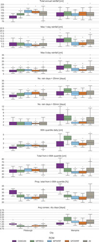
Figure A5. Correlation of selected rainfall indices to performancemetrics for the historical and future period (wetter and drier future). The top subplot (a) shows values for Pittsburgh and the bottom (b) shows values for Memphis. Grey colors represent positive correlations (from 0 to 1), while reds represent negative correlations (from 0 to —1). Labels on the left show the category of the rainfall index

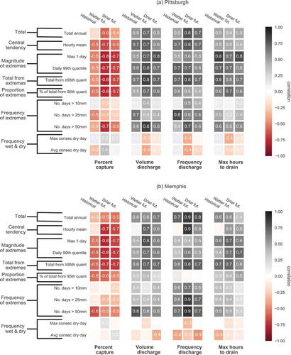
3.4. Correlation of future rain garden performance with future rainfall indices

In addition to using historical simulation results to select indices most indicative of performance, results from hydrologic simulations using future climate simulations could also be considered for rainfall index selection. This section presents correlations between the future simulated performance metrics and the rainfall indices calculated from the future climate model output for Pittsburgh.

Figure A5 presents the correlations between simulated performance and the rainfall indices for the historical and future simulations in Pittsburgh. The four performance metrics, including percent of runoff captured, volume and frequency of discharge, and maximum hours to drain the surface are shown as large columns. Each different simulation (historical, drier future, and wetter future) is shown within each large column.

Many of the same rainfall indices are correlated to the performance metrics in a similar manner as the historical simulation, but correlations generally strengthen because performance is lower. Correlations for volume discharged are slightly higher in the simulated future than in the simulated past. This could signify that as rainfall becomes more extreme, correlations will get stronger, since more volume is being discharged. Some of correlations for maximum surface drainage time in the future are weaker than they were in the historical simulations. This is likely because the time to drain is consistently higher in all years, meaning less variation across years. Thus, correlations to the rainfall indices are weaker in some cases since changes in rainfall do not change the maximum time to drain.

Overall, the rainfall indices with the strongest correlations to the performance metrics did not change considerably. Thus, examining the future correlations would not change the selection of the indices most indicative of performance, but it would validate them. As a result, it may not be necessary to consider using future simulations when developing a list of indices to track over time. However, for other locations and design configurations, this result could differ. If bias-corrected climate simulations are readily available at a sub-daily timestep, these results should be considered as part of the index selection process.

3.5. Additional factors to consider

Finally, using rainfall indices to track performance is useful if performance degrades as a result of changes in rainfall. However, these indices will not track performance degradation due to changes in infiltration as a result of clogging or poor maintenance. To track this type of performance degradation, site visits and/or compaction tests may be necessary.

References

- A&L Great Lakes Laboratories, Inc. (2015). Soil Test Report for ELPC Rain Garden Soils Taken on 2/10/2015.
- Allegheny County Sanitary Authority. (2012). ALCOSAN wet weather plan. Retrieved from http://www.alcosan.org/WetWeatherIssues/ALCOSANDraftWetWeatherPlan/DraftWWPFullDocument/tabid/176/Default.aspx
- Baltimore City Department Public Works. (2017). Stormwater remediation fee regulations. Retrieved from https://publicworks.baltimorecity.gov/sites/default/files/Stormwater%20Remediation%20Fee%20Regulations.pdf
- Bartos, M., Wong, B., & Kerkez, B. (2018). Open storm: A complete framework for sensing and control of urban watersheds. Environmental Science: Water Research & Technology, 4(3), 346–358.
- Brommer, D. M., Cerveny, R. S., & Balling, R. C., Jr. (2007). Characteristics of long‐duration precipitation events across the United States. Geophysical Research Letters, 34, L22712.
- Brown, R. A., & Hunt, W. F., III. (2010). Impacts of media depth on effluent water quality and hydrologic performance of undersized bioretention cells. Journal of Irrigation and Drainage Engineering, 137(3), 132–143.
- Bukovsky, M. (2011). Masks for the Bukovsky regionalization of North America, regional integrated sciences collective. Institute for mathematics applied to geosciences, national center for atmospheric research. Boulder, CO: University Corporation for Atmospheric Research.
- Bukovsky, M., Thompson, J. A., & Mearns, L. O. (2019). Weighting a regional climate model ensemble: Does it make a difference? Can it make a difference? Climate Research, 77(1), 23–43.
- Casal-Campos, A., Guangtao, F., Butler, D., & Moore, A. (2015). An integrated environmental assessment of green and gray infrastructure strategies for robust decision making. Environmental Science & Technology, 49(14), 8307–8314.
- CH2MHILL. (2014). Stormwater management fee policy options and recommendations. Philadelphia, PA: City of Lancaster.
- CH2MHILL, and Viridian Landscape Studio. (2011). Stormwater/Landscape Greening Project East Liberty Presbyterian Church.
- Chagrin Watershed Partners. (2017). Stormwater utility literature review. Retrieved from http://crwp.org/files/Literature_Review_by_Credit_Type.pdf
- Chapman, C., & Horner, R. R. (2010). Performance assessment of a street-drainage bioretention system. Water Environment Research, 82(2), 109–119.
- Chen, D., Achberger, C., Ou, T., Postgård, U., Walther, A., & Liao, Y (2015). Projecting future local precipitation and its extremes for Sweden. Geografiska Annaler: Series A, Physical Geography, 97(1), 25–39.
- Computational Hydraulics Int. (2018). PCSWMM. Guelph, ON: chiwater. https://www.pcswmm.com/
- Cook, L. M. (2018). Using climate change projections to increase the resilience of stormwater infrastructure designs under Uncertainty. Carnegie Mellon University.
- Cook, L. M., Anderson, C. J., & Samaras, C. (2017). Framework for incorporating downscaled climate output into existing engineering methods: Application to precipitation frequency curves. Journal of Infrastructure Systems, 23(4), 04017027.
- D’Agostino, R., & Pearson, E. S. (1973). Tests for departure from normality. Empirical results for the distributions of b 2 and√ B. Biometrika, 60(3), 613–622.
- Davis, A. P., Hunt, W. F., Traver, R. G., & Clar, M. (2009). Bioretention technology: Overview of current practice and future needs. Journal of Environmental Engineering, 135(3), 109–117.
- Davis, A. P., Traver, R. G., Hunt, W. F., Lee, R., Brown, R. A., & Olszewski, J. M. (2012). Hydrologic performance of bioretention storm-water control measures. Journal of Hydrologic Engineering, 17(5), 604–614.
- De Neufville, R., & Scholtes, S. (2011). Flexibility in engineering design. Cambridge MA and London: The MIT Press.
- Demuzere, M., Orru, K., Heidrich, O., Olazabal, E., Geneletti, D., Orru, H., … & Faehnle, M. (2014). Mitigating and adapting to climate change: Multi-functional and multi-scale assessment of green urban infrastructure. Journal of Environmental Management, 146, 107–115.
- Dietz, M. E., & Clausen, J. C. (2005). A field evaluation of rain garden flow and pollutant treatment. Water, Air, and Soil Pollution, 167(1–4), 123–138.
- Durrans, S. R., Burian, S. J., Nix, S. J., Hajji, A., Pitt, R. E., Fan, C. Y., & Field, R. (1999). Polynomial-based disaggregation of hourly rainfall for continuous hydrologic simulation. JAWRA Journal of the American Water Resources Association, 35(5), 1213–1221.
- Environmental Finance Center at the UNC School of Government. (2017). North Carolina stormwater rates and revenues - Preliminary analysis. Retrieved from https://efc.sog.unc.edu/sites/default/files/2017/NC%20Stormwater%20Chart%20Clean%202017_1_0.pdf
- Fischbach, J. R., Siler-Evans, K., Tierney, D., Wilson, M. T., Cook, L. M., & May, L. W. (2017). Robust Stormwater Management in the Pittsburgh Region.
- Foster, J., Lowe, A., & Winkelman, S. (2011). The value of green infrastructure for urban climate adaptation. Center for Clean Air Policy, 750, 19–20.
- Gregersen, I. B., & Arnbjerg-Nielsen, K. (2012). Decision strategies for handling the uncertainty of future extreme rainfall under the influence of climate change. Water Science and Technology : a Journal of the International Association on Water Pollution Research, 66(2), 284–291.
- Gregersen, I. B., Sørup, H. J. D., Madsen, H., Rosbjerg, D., Mikkelsen, P. S., & Arnbjerg-Nielsen, K. (2013). Assessing future climatic changes of rainfall extremes at small spatio-temporal scales. Climatic Change, 118(3–4), 783–797.
- Groisman, P. Y., Knight, R. W., & Karl, T. R. (2012). Changes in intense precipitation over the central United States. Journal of Hydrometeorology, 13(1), 47–66.
- Hall, A. (2014). Projecting regional change modeling regional climate change: How accurate are regional projections of climate change derived from downscaling global climate model results? Science, 34(6216), 1461–1462.
- Hathaway, J. M., Brown, R. A., Fu, J. S., & Hunt, W. F. (2014). Bioretention function under climate change scenarios in North Carolina, USA. Journal of Hydrology, 519, 503–511. doi:10.1016/j.jhydrol.2014.07.037
- Heavens, N. G., Ward, D. S., & Natalie, M. M. (2013). Studying and projecting climate change with earth system models. Nature Education Knowledge, 4(5), 4.
- IPCC. (2014). Climate change 2014: Impacts, adaptation, and vulnerability. Part A: Global and sectoral aspects. contribution of working group II to the fifth assessment report of the intergovernmental panel on climate change [Field, C.B., V.R. Barros, D.J. Dokken, K.J. Mach, M.D. Mastrandrea, T.E. Bilir, M. Chatterjee, K.L. Ebi, Y.O. Estrada, R.C. Genova, B. Girma, E.S. Kissel, A.N. Levy, S. MacCracken, P.R. Mastrandrea, and L.L. White (Eds.)]. Cambridge, UK: Cambridge University Press.
- Jennings, A. A. (2016). Residential rain garden performance in the climate zones of the contiguous United States. Journal of Environmental Engineering, 142(12), 04016066.
- Jennings, A. A., Berger, M. A., & Hale, J. D. (2015). Hydraulic and hydrologic performance of residential rain gardens. Journal of Environmental Engineering, 141(11), 04015033.
- Karl, T. R., & Knight, R. W. (1998). Secular trends of precipitation amount, frequency, and intensity in the United States. Bulletin of the American Meteorological Society, 79(2), 231–241.
- Karl, T. R., Nicholls, N., & Ghazi, A. (1999). Clivar/GCOS/WMO workshop on indices and indicators for climate extremes workshop summary. In T. R. Karl, N. Nicholls, A. Ghazi (Eds.), Weather and climate extremes (pp. 3–7). Dordrecht: Springer.
- Kerkez, B., Gruden, C., Lewis, M., Montestruque, L., Quigley, M., Wong, B., … & Poresky, A. (2016). Smarter Stormwater Systems.
- Kianfar, B., Fatichi, S., Paschalis, A., Maurer, M., & Molnar, P. (2016). Climate change and uncertainty in high-resolution rainfall extremes. Hydrology Earth System Sciences Discussions, 2016, 1–17.
- Kloss, C., Calarusse, C., & Stoner, N. (2006). Rooftops to rivers: Green strategies for controlling stormwater and combined sewer overflows. New York, NY: Natural Resources Defense Council.
- Lempert, R., & Schlesinger, M. (2001). Climate-change strategy needs to be robust. Nature, 412(6845), 375.
- McCuen, Richard. H. (2005). Hydrologic Analysis and Design. 3rd ed. Pearson Prentice Hall.
- McGinnis, S., Nychka, D., & Mearns, L. O. (2015). A new distribution mapping technique for climate model bias correction. In V. Lakshmanan, E. Gilleland, A. McGovern, & T. Martin (Eds.), Machine learning and data mining approaches to climate science (pp. 91–99). Cham: Springer.
- Mearns, L. O., McGinnis, S., Korytina, D., Arritt, R., Biner, S., Bukovsky, M., ... Gutowski, W. (2017, January 11). The NA-CORDEX dataset, version 1.0. Boulder, CO: NCAR Climate Data Gateway. doi:10.5065/D6SJ1JCH.
- Melillo, J. M., Richmond, T. T. C., & Yohe, G. W. (2014). Climate change impacts in the United States. Third National Climate Assessment, 32–37.
- Mostafavi, A. (2018). A system-of-systems framework for exploratory analysis of climate change impacts on civil infrastructure resilience. Sustainable and Resilient Infrastructure, 3(4), 175–192.
- Mustaffa, N., Ahmad, N. A., & Razi, M. A. M. (2016, July). Variations of roughness coefficients with flow depth of grassed swale. In IOP Conference Series: Materials Science and Engineering (Vol. 136, No. 1, pp. 012082). IOP Publishing.
- NOAA. (2016). National centers for environmental information. Retrieved from http://www.ncdc.noaa.gov/
- PA DEP. (2006). Pennsylvania stormwater best management practices manual. Harrisburg, PA: Bureau of Watershed Management. http://pecpa.org/wp-content/uploads/Stormwater-BMP-Manual.pdf
- Peterson, T., Folland, C., Gruza, G., Hogg, W., Mokssit, A., & Plummer, N. (2001). Report on the activities of the working group on climate change detection and related rapporteurs. World Meteorological Organization, Geneva: International CLIVAR Project Office (ICPO).
- Rawls, W. J., Brakensiek, D. L., & Miller, N. (1983). Green-Ampt infiltration parameters from soils data. Journal of Hydraulic Engineering, 109(1), 62–70. .
- Riahi, K., Rao, S., Krey, V., Cho, C., Chirkov, V., Fischer, G., … & Rafaj, P. (2011). RCP 8.5—A scenario of comparatively high greenhouse gas emissions. Climatic Change, 109(1), 33.
- Rossman, L. (2015) Storm Water Management Model User’s Manual Version 5.1 - manual. US EPA Office of Research and Development, Washington, DC, EPA/600/R-14/413 (NTIS EPA/600/R-14/413b).
- Rossman, L. A., & Huber, W. C. (2016). Storm water management model reference manual volume III – water quality. Washington, D.C.: US EPA Office of Research and Development.
- Sell, E., Beadle, K., & Read, N. (2009). Mosquitoes and rain gardens: An update. St. Paul, MN: Metro Mosquito Control District.
- Thakali, R., Kalra, A., Ahmad, S., & Qaiser, K. (2018). Management of an urban stormwater system using projected future scenarios of climate models: A watershed-based modeling approach. Open Water Journal, 5(2), 1.
- U.S. EPA. (2016, June 19). “What is green infrastructure?” Green infrastructure. Retrieved from https://www.epa.gov/green-infrastructure/what-green-infrastructure
- Wadzuk, B. M., Lewellyn, C., Lee, R., & Traver, R. G. (2017). Green infrastructure recovery: Analysis of the influence of back-to-back rainfall events. Journal of Sustainable Water in the Built Environment, 3(1), 04017001.
- Washington State Legislature. (2000). Chapter 173-245 wac submission of plans and reports for construction and operation of combined sewer overflow reduction facilities. Retrieved from https://apps.leg.wa.gov/WAC/default.aspx?cite=173-245&full=true#173-245-080
- Westra, S., Fowler, H. J., Evans, J. P., Alexander, L. V., Berg, P., Johnson, F., … & Roberts, N. M. (2014). Future changes to the intensity and frequency of short-duration extreme rainfall. Reviews of Geophysics, 52(3), 522–555.
- William, R., Gardoni, P., & Stillwell, A. S. (2018). Reliability-based approach to investigating long-term clogging in green stormwater infrastructure. Journal of Sustainable Water in the Built Environment, 5(1), 04018015.
- Zhang, K., Manuelpillai, D., Raut, B., Deletic, A., & Bach, P. M. (2019). Evaluating the reliability of stormwater treatment systems under various future climate conditions. Journal of Hydrology, 568, 57–66.