Geographic Isolation and Vulnerability Across Peru’s Ecological Regions: The Influence of Regional Contexts of Extraction

Abstract

Geographically isolated places are often sites of exported environmental risks, intense resource extraction, exploitation and marginalization, and social policy neglect. These conditions create unique challenges related to vulnerability and adaptation that have direct disaster management implications. Our research investigates the relationship between geographic isolation and flood-related social vulnerability across Peru’s ecological regions. Ecoregions have different relationships with colonialism and capitalism that shape vulnerability, and we hypothesize that the relationship between vulnerability and geographic isolation varies across ecoregions. Using mapping techniques and spatial regression analysis, we find that relationships between vulnerability and geographic isolation vary regionally, with differences that suggest alignment with regional contexts of extraction. We find notable differences in vulnerability related to public health infrastructure and access to services and between ecoregions with sharply contrasting histories of natural resource extraction and investment and disinvestment.

地理上与世隔绝的地方往往具有这些特点: 外来环境风险、资源密集开采、剥削和边缘化、被社会政策所忽视。这些条件造成了脆弱性和适应的独特挑战, 对灾害管理产生直接影响。本文研究了秘鲁生态区的地理隔绝与洪水社会脆弱性之间的关系。生态区与殖民主义和资本主义的不同关系塑造了脆弱性。本文假设脆弱性和地理隔绝的关系因生态区域而异。通过制图和空间回归分析, 发现脆弱性和地理隔绝的关系在不同区域确有差异, 而这些差异与资源开采的区域背景相一致。公共卫生基础设施和获取服务, 以及拥有不同自然资源开采、投资和撤资历史的各个生态区域, 都存在着脆弱性上的显著差异。

Los lugares geográficamente aislados son a menudo sitios de riesgos ambientales exportados, intensa extracción de recursos, explotación y marginación, y olvidados en las políticas sociales. Estas condiciones crean retos únicos relacionados con vulnerabilidad y adaptación, que tienen implicaciones directas en el manejo de desastres. Nuestra investigación versa sobre la relación entre el aislamiento geográfico y la vulnerabilidad social, asociada con las inundaciones en todas las regiones ecológicas del Perú. Las ecorregiones tienen diferentes relaciones con el colonialismo y el capitalismo que dan forma a la vulnerabilidad, y al respecto hipotetizamos que la relación entre la vulnerabilidad y el aislamiento geográfico varía a través de las ecorregiones. Usando técnicas de mapeo y análisis de regresión espacial, encontramos que las relaciones entre la vulnerabilidad y el aislamiento geográfico varían regionalmente, con grados de diferencia que sugieren un alineamiento con contextos regionales de extracción. Hallamos notables diferencias en la vulnerabilidad relacionada con la infraestructura de la salud pública y el acceso a los servicios, y entre ecorregiones con historias muy contrastadas de la extracción de los recursos naturales e inversión y desinversión.

Key Words:

• ecological regions
• geographic isolation
• resource extraction
• spatial regression
• vulnerability

关键词:

• 生态区
• 地理隔离
• 资源开采
• 空间回归
• 脆弱性

Palabras clave:

• aislamiento geográfico
• extracción de recursos
• regiones ecológicas
• regresión espacial
• vulnerabilidad

As climate change continues to impact the habitability of spaces and the probability of adverse events increases, understanding spatial distributions of vulnerability is critical. Spatial constructs related to geographic isolation have garnered less attention in disaster research, however, despite the greater overall vulnerability of rural areas and heterogeneity in these areas’ resilience (Cutter, Ash, and Emrich 2016). Geographic isolation is shaped by globalization and community responses to globalization, including varying histories of investment and disinvestment and different relationships with social and economic drivers of vulnerability (LeFebvre 1991, 46–49, 343–47; Massey 2005; Meyfroidt et al. 2013). Geographically isolated populations might face less-diversified economic opportunities, poorer access to health and education services, and higher transportation costs and limited accessibility that restrict emergency aid and adaptation options (Shultz et al. 2016; Doogan et al. 2018). On the other hand, geographically isolated populations could have particularly strong communal support networks and histories of adaptation and resilience that are protective (Fitzhugh 2012).

To investigate associations between geographic isolation and vulnerability, we examine regional heterogeneity in this relationship based on the understanding that different social and historical contexts and different levels and types of extraction between natural settings (e.g., different extractive systems between industrial and ecological regions) shape the political and economic conditions that underpin vulnerability (Bunker 1988; Tickamyer and Patel-Campillo 2016; Pearce 2020). Regions are created by social and economic processes tied to neoliberal growth and degrowth and thus can be divided by areas of industrial production and extraction (e.g., coal-mining areas; Massey 1983; Allen, Massey, and Cochrane 2012). Effects of this regionalization might last long after place-specific economic activity ends, as social, economic, and political shifts related to the closing of mining operations, for example, could follow regional patterns (Massey 1983). Foundational spatial research has weighed social and economic contexts to investigate regional interactions and rebuff the “constancy assumption,” which states that a relationship observed among all units also applies to individual units (Freedman et al. 1991; O’Loughlin, Flint, and Anselin 1994). This research has used mapping and spatial regression to explore regional differences and the role of local social and economic factors in shaping spatial differentiation (O’Loughlin, Flint, and Anselin 1994; Curtis, Voss, and Long 2012; Autant-Bernard and LeSage 2019). We offer similar contextual scrutiny. Peru’s ecological regions (ecoregions) reflect social, economic, political, and cultural differences linked to legacies of colonialism and resource-specific extractive racial capitalism (Pearce 2020). Considering intertwined social and environmental histories and the role of wider contexts in shaping space (Sharkey and Faber 2014), we approach regions as socioecological regions and hypothesize that leading aspects of vulnerability and the relationship between vulnerability and geographic isolation vary across ecoregions according to regional experiences with extraction. Through this analysis, we aim to offer a nuanced understanding of vulnerability and geographic isolation in Peru useful to spatial researchers and disaster response professionals alike.

Context of Geographic Isolation and Socioecological Regions in Peru

From the Spanish conquest of the Inca Empire in the early to mid-1500s, colonialism in Peru was primarily concerned with commodity production, and spatial attention shifted depending on commodities’ global importance. Extraction was organized regionally: sugar and cotton cash crops from the north and central coast, minerals from the Andes, oil from the north coast, wool from the southern highlands, and rubber from the Amazon (Fallaw and Nugent 2020, 32). Following independence in 1821, the Lima and coastal plantation-based elite continued to regard Peru’s interior as a source of wealth to support the new country’s development and the interior’s overwhelmingly Indigenous population as a source of labor for this extraction (Medd and Guyot 2019; Fallaw and Nugent 2020, 26–30). The more remote Amazon and Andes regions were sites of particularly intense extraction. The rubber boom of the late nineteenth and early twentieth centuries quickly reduced the Amazon’s geographic isolation via transportation infrastructure necessary for extraction as new cities like Iquitos grew to support related industries and long supply chains (Tully 2011, 67–68). Destructive mining operations and related environmental risks and social and economic consequences were, and continue to be, primarily located in the Andes (see Figure 1 in Edraki and Unger 2015). Compounding effects of historic and ongoing extractive activity, rural development policies have exacerbated inequality in more geographically isolated places, particularly in interior ecoregions (Flachsbarth et al. 2018).

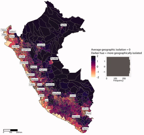
Figure 1. Travel time to nearest city of 50,000 (Nelson 2008).

Vulnerability Construct and Flood Hazards

In this study, we examine a vulnerability construct related to flood hazards. We focus on floods for illustration purposes, using a conceptualization of social vulnerability pertinent to a common hazard in Peru to assess spatial differentiation of vulnerability. Researchers have proposed many definitions and conceptualizations of vulnerability, many similar and some conflicting (Cutter 1996). Recent classifications differentiate vulnerability as susceptibility to adverse impacts from hazards and social vulnerability as susceptibility to adverse impacts as determined by a community’s sociodemographic and economic properties (Wang et al. 2021). Drawing on seminal social vulnerability indexes (Cutter, Boruff, and Shirley 2003), recent research also stresses the wide range of conditions that might be considered as influencing social vulnerability, including health status, socioeconomic status and access to social assistance, housing conditions and the built environment, and gender, age, race, ethnicity, and language (Tuccillo and Spielman 2022). We conceptualize social vulnerability through such an inclusive lens and approach susceptibility to hazards’ adverse impacts as overwhelmingly a social calculus (Smith 2006), closely linked to colonial legacies and globalization (O’Brien and Leichenko 2000; Bonilla and LeBrón 2019). As we approach susceptibility as largely socially determined, we also approach vulnerability as overwhelmingly social. This social emphasis reflects recent calls for flood vulnerability research to investigate mechanisms driving disparities in impacts (Hino and Nance 2021).

Vulnerability research has considered factors relevant to geographic isolation. Research examining rural vulnerability has found that vulnerability in rural places can be created and exacerbated by highly subsistence economies with few food alternatives (Birkmann and Wisner 2006), dependence on a single economic source (Bach 2017), and strong positive associations with other social vulnerability factors, such as low employment and education, poor housing quality, high poverty, and large numbers of racial and ethnic minoritized groups (Cutter and Emrich 2006; Lee et al. 2021). Also related to geographic isolation, recent flood-related vulnerability research has investigated relationships between vulnerability and access to resources, amenities, markets, and services critical in responding to flood events (Bashier Abbas and Routray 2014; Jamshed et al. 2020). This recent research finds higher overall social vulnerability in geographically “remote” areas and links greater risks of severe health and livelihood impacts in rural areas farther from cities to weaker services and facilities (Bashier Abbas and Routray 2014; Mavhura, Manyena, and Collins 2017; Jamshed et al. 2020). Similarly, and more local to our research case, research on flood vulnerability in Arequipa, Peru, has examined relationships between distance to emergency resources and vulnerability at the city block level (Thouret et al. 2013). We build on this research, assessing how various aspects of vulnerability relate to geographic isolation in different regional contexts. Investigating the relationship between vulnerability and geographic isolation has crucial disaster management implications, as research can identify types of vulnerability more common in geographically isolated contexts, as well as sources of vulnerabilities, which support policy interventions.

Regional differences in hazard exposure and cumulative risk do not factor into our spatial analysis of vulnerability, yet varying flood types and mechanisms across Peru offer important background (Fekete 2009; Chang and Chen 2016). Floods on the west side of the Andes are rapid onset, often resulting in flash floods, and are typically associated with extreme precipitation and El Niños (anomalously warm ocean temperatures in the equatorial Pacific; Poveda et al. 2020). In the Andes, glacial retreat and the corresponding growth of glacial lakes increases flood risk and related avalanche and landslide risks (Huggel et al. 2020). In the Amazon, flood extremes are often linked to La Niña conditions (anomalously cold ocean temperatures in the equatorial Pacific) and typically evolve slowly due to large watersheds and long rivers. As elsewhere in the country, floods in the Amazon have devastating impacts on health, safety, and food security, but annual flood cycles are also critical to sustaining Amazon livelihoods (Marengo and Espinoza 2016; Sherman et al. 2016).

Data and Measures

Indicator of Geographic Isolation

We operationalize geographic isolation as travel time to the nearest city to reflect factors like transportation routes and infrastructure relevant to both historic and current extraction and access to services and emergency aid. Isolation by distance is the simplest way to delineate geographic isolation, where greater distance between points increases relative geographic isolation (Holman et al. 2007). Natural barriers, land surface types, and changes in altitude, however, increase travel difficulties (White and Barber 2012), and few transit links and high travel costs reduce accessibility (Roy, Schmidt-Vogt, and Myrholt 2009). These connectivity-related characteristics included in our operationalization reflect ease of interaction between places.

We use an indicator for travel time to nearest city created by the European Commission (Nelson 2008). The indicator considers transportation networks and environmental and political factors to estimate travel time to the nearest city of 50,000 inhabitants (Uchida and Nelson 2010). Transportation networks include roads and railways and navigable rivers. Environmental factors include land cover and slope. Population distribution within units is partially accounted for using spatial data, including, for example, land cover and distance to roads, which increases measure precision to the 1 km pixel level (Uchida and Nelson 2010). The measure does not, however, consider transportation cost differences and economic disparities between places, which could affect travel accessibility (Roland and Curtis 2020). The indicator is pertinent to disaster management and flood risk, and the indicator’s implied availability or absence of emergency facilities and services is used to measure disaster-coping capacity in the Red Cross 510 dashboard.¹

Figure 1 depicts the geographic isolation metric by district. Gray lines represent district boundaries. District-level distinctions were selected for the geographic isolation metric and vulnerability indicators as districts are the smallest administrative subdivision in Peru, after provinces and regions, and the smallest scale for which data are available. District population size varies between regions as regions historically required different population minimums for the creation of new districts (Instituto Nacional de Estadistica e Informatica 1993). Peru has 1,832 districts, but data include 1,873 divisions as some districts are split in the data. This additional number of divisions increases spatial specificity. Darker shades and larger numbers represent longer travel time to the nearest city and greater geographic isolation. Travel time ranged from 0 minutes (many districts) to 4,099 minutes (Soplin district in the Amazon), with an average of 461 minutes (in Figure 1, a geographic isolation score of 0 represents this national average). We scaled and normalized geographic isolation data using z scores, which supports comparisons with vulnerability characteristics normalized using the same procedure. This operationalization assumes that different changes in travel time (e.g., 0–20 minutes compared to 40–60 minutes) have the same effect on geographic isolation. To prevent outliers from skewing visualization, we set limits at two standard deviations from the mean (± 2). All indicator and vulnerability maps in this study follow similar visualization procedures. The global Moran’s I using rook contiguity is 0.68 (p < 0.001), indicating strong positive spatial autocorrelation (i.e., travel time is similar among districts neighboring one another).

Vulnerability Indicator Identification and Reduction

Vulnerability studies typically build an index of vulnerability indicators from stakeholder input and literature that empirically links indicators with impacts (Cutter, Boruff, and Shirley 2003). We followed the same approach. To identify relevant indicators, we drew on vulnerability frameworks and indexes that emphasize social, economic, institutional, and cultural dimensions of vulnerability (see the MOVE framework in Jamshed et al. 2019), livelihood influences (see the Sustainable Livelihoods framework in Birkmann 2013), and health vulnerability (Bashier Abbas and Routray 2014). We ranked indicators using an iterative case study and multimodel approach to gather stakeholder feedback. Our study is part of a larger collaboration with partners at the Red Cross Red Crescent Climate Center and German Red Cross in Peru. Discussions with these partners, a site visit to Iquitos, a three-day workshop with flood disaster professionals in Lima in June 2019, and follow-up interviews with workshop attendees informed indicator selection. An online survey of flood disaster professionals in Peru conducted in December 2019 and January 2020 was used to rank indicators. Survey respondents were recruited via e-mail from a list of workshop attendees and the professional networks of the Red Cross Red Crescent Climate Center and the German Red Cross in Peru. The convenience sample encompassed the range of stakeholders involved in disaster preparedness and response in Peru. Of the approximately 150 stakeholders e-mailed, fifty-six responded and thirty-six completed most of the survey, yielding a 0.37 response rate.² Flood disaster professionals assigned the greatest importance to health- and poverty-related indicators. Further results, including differences in perceptions related to respondents’ field of work and geographic location, can be found in our survey report (Roland et al. 2021).

We present indicators used in our construct of flood-related social vulnerability in Peru in Table 1, including a rationale for indicator selection, the rank in the survey of flood disaster professionals, and a hypothesized relationship, positive or negative, with vulnerability. Indicators fall within five categories of vulnerability: built environment, demographic, education, health, and socioeconomic. Our district-level vulnerability data are from the 2017 Peru national census and the Red Cross 510 data set, a compilation of risk assessment data by the Netherlands Red Cross (Peru Instituto Nacional de Estadísticañ e Informática 2017; 510 The Netherlands Red Cross, 2020). Like other studies (Oulahen et al. 2015), we scaled and normalized data using z scores to compare data with different scales. This process created vulnerability data with means of 0 and standard deviations of 1.

Table 1. Flood-related vulnerability indicators

Vulnerability category	Vulnerability indicator	Rationale for inclusion	+ or – relationship with vulnerability	Flood disaster professionals ranked level of importance (1 = most important)
Built environment	Percentage of households without public water supply	Piped water from a public water supply is safer than surface water	+	5.0
	Percentage of households without sewage infrastructure	Households lacking sewage infrastructure are at higher risk of communicable diseases	+	7.5
	Percentage of households without strong walls	Homes without strong walls are more likely to suffer flood damage	+	14.0
	Percentage of households without electricity	Electricity is a proxy for wealth and connectivity related to information and media and home accessibility	+	16.5
Demographic	Percentage elderly (> 65) and children (< 5)	Children and elderly are less mobile and have greater health risks	+	4.0
	Household size	Greater family size could increase vulnerability, although isolated individuals might have weaker social supports	+	12.0
	Infant mortality rate	Infant mortality rate is related to numerous vulnerability-exacerbating social, economic, and environmental factors including infectious disease prevalence and poor sanitation and health infrastructure	+	13.0
	Percentage with disability	Populations with disabilities are less mobile and particularly vulnerable to natural hazards and health risks	+	16.5
	Life expectancy	Lower life expectancy suggests a more vulnerable elderly population	–	19.0
	Percentage women	Women receive lower wages and have more family care responsibilities	+	20.0
Education	Percentage illiterate	Literacy is closely related to socioeconomic status and lifetime earning potential as well as access to information	+	6.0
	Percentage who have not completed primary education	Education is closely related to socioeconomic status and lifetime earning potential	+	7.5
	Percentage without a college degree	Education is closely related to socioeconomic status and lifetime earning potential	+	11.0
	Number of educational facilities per 10,000 people	More education facilities increase proximity and access	–	15.0
Health	Waterborne disease incidence	Higher waterborne disease incidence indicates higher baseline health risks directly related to floods and suggests prior flood events	+	1.0
	Percentage child malnutrition	Child malnutrition is related to numerous vulnerability-exacerbating social, economic, and environmental factors including extreme poverty and access to food	+	3.0
	Number of health facilities per 10,000 people	More health facilities increase proximity and access to care	–	9.5
	Percentage with health insurance	Uninsured populations are less able to receive health care, even if accessible	–	9.5
Socioeconomic	Poverty rate	Wealth enables both better protection from hazards and recovery from losses	+	2.0
	Percentage of homes that are rented	Renters are less able to take mitigative steps and are more likely to be transient and have fewer financial resources	+	18.0

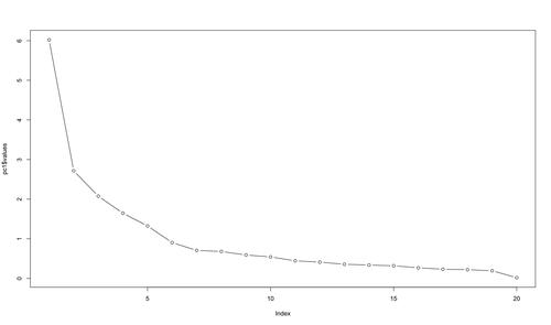
To reduce this large number of indicators to a smaller number of new variables that reflect different aspects of vulnerability, we used a principal component analysis (PCA; Cutter, Boruff, and Shirley 2003). Using a varimax rotation to increase the variation between each new factor (Cutter, Boruff, and Shirley 2003), we identified six components using a scree plot (see Appendix A for plot). These components, depicted in Table 2, explained 73 percent of the variation in vulnerability among districts.

Table 2. Vulnerability components and indicator loading

Component	% of variance	Weight calculated from survey of flood disaster professionals	Principal indicators	Correlation
1. Wealth	23	0.0616	Literacy	0.85
			Primary education completion	0.84
			Poverty	0.79
			Percentage with health insurance	–0.72
			College completion	0.68
			Percentage of homes that are rented	–0.67
			Child malnutrition	0.63
			Access to sewage system	0.51
2. Public health infrastructure	13	0.0488	Access to public water supply	0.88
			Access to electricity	0.75
			Access to sewage system	0.70
			House construction materials	0.53
3 Demographic (± adjustment)	12	0.0484	Household size	–0.81
			Percentage with a disability	0.80
			Percentage elderly (> 65) and children (< 5)	0.76
4. Health	10	0.0238	Life expectancy	0.88
			Infant mortality rate	0.83
5. Access to services (± adjustment)	10	0.0595	Hospitals per 10,000 people	–0.78
			Waterborne disease incidence	0.78
			Educational facilities per 10,000 people	–0.58
6. Gender	6	0.0048	Gender	0.91

Following a PCA, the most common next step in vulnerability analysis is to combine components in an additive model to create a composite vulnerability score (Cutter, Boruff, and Shirley 2003). Expert input is typically only integrated in earlier indicator-selection steps, which leads composite vulnerability measures to be viewed as insufficiently grounded in local perceptions of vulnerability (Fekete 2012). Indexes informed by local experts are more likely to accurately reflect local contexts and are perceived as more transparent than indexes not informed by local experts (Oulahen et al. 2015; Beccari 2016). To integrate expert input more fully into our analysis, we build on research that uses stakeholders to validate data-driven outputs (Oulahen et al. 2015; Alvarez et al. 2018) and that follows PCA with further statistical analysis using stakeholders’ indicator ratings (Mascarenhas, Nunes, and Ramos 2015). We use indicator rankings from our survey of flood disaster professionals to weight PCA components that make up the overall vulnerability score by stakeholders’ perceptions of the importance of each of the principal indicators within the component. Although this approach only applies to our measure of overall vulnerability, it means that, rather than simply summed, components are combined in a way that accounts for expert input. In creating a measure of overall vulnerability that uses input from flood disaster professionals to weight vulnerability domains derived from the widely used PCA method, we offer an innovative approach that integrates these common, yet typically separate, methods of indicator development and is both data-driven and informed by local experts. Although the survey of flood disaster professionals was designed to evaluate the importance of individual indicators, we adapt individual indicator rankings to weight the PCA’s six components. To do so, we first calculate proportional weights for each indicator according to $$w_i=\mathrm{ }\frac{n-r_i+1}{\sum (\mathrm{n}-r_i+1)},\mathrm{ }$$ where w_i is the weight for vulnerability indicator i, n is the total number of indicators in the index, and r_i is the ranked position of indicator i (Oulahen et al. 2015). Weights sum to 1. Using these individual indicator weights, we create component weights by calculating the average weight of the individual indicators that load as principal indicators on each component. For example, for the health component that includes infant mortality rate and life expectancy as principal indicators, we calculate the average weight from the survey of these two indicators. We then multiply this average weight by component scores before adding components to create the composite score. This process follows $$v_k=\mathrm{ }\sum _{j=1}^n{x}_{kj}\left(\frac{\sum _{i=1}^{n_j}{w}_i}{n_j}\right),\mathrm{ }$$ where v_k is the vulnerability composite for district k, x_kj is the component score for district k and component j, w_i is the weight for vulnerability indicator i, and n_j is the number of indicators in component j.

Ecological Regions

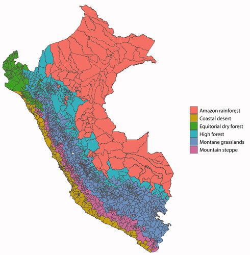
We use ecoregions as a proxy for different experiences with extraction, liberalization, and disinvestment to consider the influence of social and economic conditions on varying relationships between vulnerability and geographic isolation. We thus approach ecoregions as socioecological regions. To investigate this regional heterogeneity, we use a variable for ecoregions from the Ministry of Environment of Peru (2017) that originally included nine ecoregion types. Because ecoregions do not align with district boundaries, we intersected the ecoregion map with district boundaries and defined district-level ecoregion according to the ecoregion type with the greatest proportion of the district’s land area. Almost all districts fall within six ecoregions (Figure 2): equatorial dry forests (131 districts), coastal deserts (203 districts), mountain steppes (256 districts), montane grasslands (803 districts), high forests (360 districts), and the Amazon rainforest (120 districts). Two districts fell within other ecoregions and were subsumed into surrounding ecoregions to be statistically represented. Comparing geographic isolation and ecoregion maps (Figures 1 and 2) indicates substantial variation in geographic isolation between ecoregions, which supports investigation into relationship variation between geographic isolation and vulnerability by ecoregion.

Figure 2. Ecoregions of Peru (Ministry of Environment of Peru 2017).

Method

Mapping Vulnerability Characteristics

Assessing the relationship between vulnerability and geographic isolation across Peru requires first understanding where different aspects of vulnerability matter most. In our first analytical step, we map survey-informed composite vulnerability, vulnerability components, and the individual indicators that flood disaster professionals ranked highest. Like other visualizations, these maps, presented in Figures 3 and 4, center around a national mean of 0 and have limits at two standard deviations from the mean (± 2). Darker hues indicate greater vulnerability.

Figure 3. Spatial distribution and local Moran’s I of the principal components analysis (PCA) vulnerability composite informed by flood disaster professionals and PCA components of vulnerability.

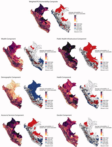
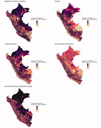
Figure 4. Spatial distribution of vulnerability for the five indicators rated most important in the survey of flood disaster professionals in Peru.

To identify spatial clustering of high and low vulnerability (e.g., districts with high vulnerability and high vulnerability in neighboring districts), we map the local Moran’s I for composite vulnerability and vulnerability components, also presented in Figure 3 (Anselin 1995). We selected a rook contiguity matrix to construct the spatial weights matrixes identifying neighboring districts. In this matrix, each neighboring district is allocated equal weight. Statistically significant high spatial autocorrelation is often used to select a spatial weights matrix (Chi and Zhu 2019, 40), and rook contiguity produced the greatest global Moran’s I statistics for overall vulnerability compared with queen contiguity and various distance and nearest neighbors criteria. Rook and queen contiguity are also common in social vulnerability spatial analysis (Gaither et al. 2011; Frigerio and De Amicis 2016; Hou et al. 2016), and rook contiguity is sometimes favored for its more stringent application of polygon contiguity (Frigerio and De Amicis 2016). In Peru, where district size and distance between districts vary widely, this conservative approach is appropriate as it reduces chances of overstating the geographic reach of spatial patterns.

Spatial Regression Analysis

The second step in our analysis uses spatial regression to evaluate variation in the relationship between geographic isolation and vulnerability across Peru’s ecoregions. Our comparative results emphasize the specific spatial context of our study and allow for interpretation in terms of how regions relate to each other, including contrasting regional historical and social contexts, based in our relational approach to space (Massey 2013). A spatially informed analysis is important because districts are interdependent: Characteristics of one district affect those of neighbors (Tobler 1979; Getis and Ord 1992). Vulnerability is determined not only by resources and services in a district but also by resources and services in neighboring districts (e.g., a person in one district might access medical care in a neighboring district) and by interactions between districts (e.g., a person in one district might lend support to residents of a neighboring district; Voss, Curtis White, and Hammer 2006). Contiguous districts also have similarities, as district boundaries do not reflect abrupt differences in social and geographic characteristics or histories of extraction (Tolnay, Deane, and Beck 1996). Measures of spatial autocorrelation confirm our theoretical basis for spatial regression. The global Moran’s I statistic and global Geary’s C statistic find statistically significant strong positive spatial autocorrelations for vulnerability measures. We generate our spatially lagged variable, representing average vulnerability in neighboring districts, by multiplying spatial weights from our spatial weights matrix by vulnerability scores and summing for all neighbors (Anselin 1989).

We use a spatial autocorrelation (SAC) regression model to regress vulnerability components, as well as the vulnerability composite, on geographic isolation with a dummy variable for ecoregion and an interaction term for geographic isolation and ecoregion (Chi and Zhu 2019). A SAC model includes spatial autocorrelation for the dependent variable, vulnerability, and the error term. Given the theoretical basis for spatial scrutiny of vulnerability in neighboring districts, assessing the spatial dependence of vulnerability is essential. The SAC model has the smallest Akaike’s information criterion values for the vulnerability composite and for all components compared to spatial lag, spatial error, spatial Durbin, and ordinary least squares (OLS) nonspatial models, suggesting that the SAC model best fits the data. We ran our analysis with the alternative models and found no substantive difference in results (Anselin 1999, 11; LeSage and Pace 2009, 23, 28–29; see Appendix B for equations and results of alternative models). We ran the model separately for overall vulnerability, as determined by the flood disaster professional-weighted PCA composite, as well as each PCA component. The interaction term is the crux of our analysis as it assesses the conditioning force of ecoregion on the relationship between vulnerability and geographic isolation. The model is expressed in the equation $$Y_i=\alpha \mathrm{ }{+\mathrm{ }\rho {\sum }_j{Y_{j}W}_j+\beta }_1{X}_i+{{\beta }_{2}Z}_i+{{\beta }_{3}X}_i\mathrm{*}{Z}_i+\mathrm{ }u,$$ $$u=\lambda {\sum }_j{u_{j}W}_j+{\epsilon }_i,\mathrm{ }$$ where Y_i is the vulnerability of district i, α is the regression constant, $\rho$ is the strength of the association with extralocal vulnerability holding district vulnerability constant, Y_j is the vulnerability of extralocal district j, W_j is the proximity of district j to district i as determined by the spatial weights matrix, β₁ is the strength of the association with district geographic isolation, X_i is the geographic isolation of district i, β₂ is the strength of the association with ecoregion, Z_i is the ecoregion of district i, β₃ is the strength of the association with the interaction between geographic isolation and ecoregion, $u$ is error and extralocal error, $\lambda$ is the strength of the association with extralocal error, $u_j$ is the error term for extralocal district j, and ε_i is the error term for district i.

Results

Spatial Distribution of Vulnerability

Visualizations of flood-related social vulnerability show spatial patterns aligning with ecoregion and geographic isolation that suggest regional variation in the relationship between vulnerability and geographic isolation. For overall vulnerability, we observe positive associations between vulnerability and interior, and generally more isolated, ecoregions, as well as between vulnerability and more geographically isolated districts within ecoregions. High overall vulnerability clusters in the interior mountain steppe and montane grasslands Andes ecoregions and the Amazon ecoregion where intense extractive activities have been, and continue to be, concentrated. Across the country, lower overall vulnerability clusters around large cities like Iquitos, Tarapoto, Huancayo, Ayacucho, and Cusco.

Component maps illustrate where specific aspects of vulnerability matter most, which can inform our understanding of relationships between different types of vulnerability and geographic isolation, as well as possible regional variation in these relationships. Correlations with geographic isolation are noticeable in most components. In the wealth component, low-vulnerability clusters are primarily found around large cities, and particularly coastal cities like Lima, Pisco, and Arequipa. Similarly, in the public health infrastructure component, the cities of Iquitos and Pucallpa are not included in the high-vulnerability cluster that makes up much of the Amazon ecoregion. Mapping component vulnerability also reveals clustering by ecoregion. High vulnerability in numerous components concentrates in Amazon and montane grassland and mountain steppe Andes districts. For example, high wealth-related vulnerability clusters in the montane grasslands and high forest ecoregions that border the Andes on the east, high vulnerability related to accessing to services clusters in the Amazon and mountain steppe ecoregions, and high public health infrastructure-related vulnerability clusters in the Amazon ecoregion. In contrast, low vulnerability in wealth and health-related components clusters in coastal desert districts.

Mapping individual indicators helps probe sources of spatial difference in component vulnerability. Maps of individual indicators that flood disaster professionals rated as most important (i.e., waterborne disease, poverty, child malnutrition, percentage elderly and children, and access to public water indicators most important) emphasize that key attributes of flood-related social vulnerability concentrate in interior regions, particularly the Amazon and montane grassland and mountain steppe Andes ecoregions. Poverty and child malnutrition concentrate in the Amazon and montane grassland ecoregions. Access to public water heavily concentrates in Amazon districts and, to a lesser extent, select districts in the mountain steppe ecoregion. Sewage infrastructure shows similar regional differences. Vulnerability related to elderly and young populations is highest in the more geographically isolated mountain steppe ecoregion. Waterborne disease incidence concentrates in Amazon, mountain steppe, and coastal desert ecoregions.

Spatial Regression Results

Having established a spatially informed understanding of vulnerability in Peru, we use spatial regression to empirically assess regional differences in the relationship between geographic isolation and vulnerability. Crucially, the interaction term in our model, between geographic isolation and ecoregion, estimates differentiation across ecoregions. The coefficients presented in Table 3 reflect the direct association of the immediate district rather than the net association that includes the influence of neighboring districts. The rho (spatial autoregressive coefficient) describes the influence of the outcome variable among all neighboring districts. Statistically significant and mostly positive rho values confirm the importance of a spatial structure. Positive rho values ranging from 0.7 to 0.9 in overall vulnerability and all components but health reflect strong positive spatial feedback where vulnerability is more similar between neighboring districts than between nonneighboring districts.

Table 3. Spatial regression results: Spatial autocorrelation (SAC) model

		Vulnerability components
	Overall vulnerability	Wealth	Public health infrastructure	Demographic	Health	Access to services	Gender
Constant	–0.629*** (0.133)	–0.261* (0.109)	–0.448*** (0.121)	–0.023 (0.119)	–0.018 (0.211)	–0.291* (0.121)	–0.019 (0.159)
Travel time to city (TT)	0.528*** (0.096)	0.157* (0.078)	0.496*** (0.089)	–0.137 (0.085)	–0.005 (0.122)	0.306*** (0.087)	0.038 (0.112)
Coastal desert	0.290 (0.185)	0.166 (0.154)	0.644*** (0.171)	–0.056 (0.168)	–1.105*** (0.244)	–0.010 (0.170)	–0.025 (0.224)
Equatorial dry forest	0.828*** (0.154)	0.445*** (0.127)	0.474*** (0.140)	0.060 (0.138)	–0.208 (0.225)	0.407** (0.139)	–0.142 (0.183)
High forest	0.624*** (0.137)	0.282* (0.113)	0.377** (0.125)	0.040 (0.123)	0.031 (0.181)	0.283* (0.124)	–0.061 (0.163)
Montane grasslands	0.690*** (0.135)	0.298** (0.111)	0.444*** (0.122)	0.064 (0.121)	0.066 (0.187)	0.260* (0.122)	0.104 (0.160)
Mountain steppe	0.743*** (0.137)	0.198 (0.112)	0.455*** (0.124)	0.226 (0.125)	–0.053 (0.199)	0.391** (0.124)	–0.151 (0.163)
TT × Amazon	Reference	Reference	Reference	Reference	Reference	Reference	Reference
TT × Coastal desert	–0.456*** (0.135)	–0.105 (0.112)	–0.270* (0.125)	0.176 (0.123)	–0.084 (0.160)	–0.456*** (0.125)	–0.174 (0.164)
TT × Equatorial dry forest	–0.163 (0.120)	0.027 (0.100)	–0.380*** (0.111)	0.206 (0.109)	0.013 (0.158)	–0.125 (0.110)	–0.149 (0.145)
TT × High forest	–0.456*** (0.101)	–0.113 (0.082)	–0.334*** (0.092)	0.057 (0.089)	–0.082 (0.128)	–0.272** (0.091)	–0.077 (0.119)
TT × Montane grasslands	–0.439*** (0.097)	–0.082 (0.080)	–0.482*** (0.090)	0.115 (0.087)	–0.026 (0.126)	–0.252** (0.088)	–0.132 (0.116)
TT × Mountain steppe	–0.269** (0.103)	–0.069 (0.085)	–0.470*** (0.097)	0.332*** (0.094)	0.017 (0.133)	–0.204* (0.095)	–0.150 (0.124)
Rho	0.764***	0.889***	0.860***	0.861***	–0.298***	0.877***	0.724***
Lambda	–0.355***	–0.515***	–0.602***	–0.456***	0.885***	–0.654***	–0.529***
AIC	4,002	3,715	4,197	3,885	3,689	4,298	4,941

Note: Standard errors are reported in parentheses. AIC = Akaike’s information criteria.

*p < 0.05.

**p < 0.01.

***p < 0.001.

Our model finds clear differences in the relationship between vulnerability and geographic isolation across ecoregions, particularly between ecoregions with contrasting levels of investment and experiences with extraction. For overall vulnerability, geographic isolation is most associated with higher vulnerability in the Amazon reference region. Compared to the Amazon region, geographic isolation is least associated with higher overall vulnerability in the coastal desert (–0.456), high forest (–0.456), and montane grasslands (–0.439) ecoregions. We see similar regional differences in component vulnerability. The most striking regional differences emerge in the public health infrastructure and access to services domains and between Amazon and coastal desert ecoregions, which represent regional extremes in Peru in terms of historic and current extractive activity and investment and disinvestment. Geographic isolation more strongly associates with higher public health infrastructure-related vulnerability in the Amazon reference region than in other ecoregions. Compared to the Amazon region, geographic isolation associates more weakly with higher public health infrastructure-related vulnerability in the coastal desert (–0.270), equatorial dry forest (–0.380), high forest (–0.334), montane grasslands (–0.482), and mountain steppe (–0.470) ecoregions. In the access to services vulnerability domain, geographic isolation again more strongly associates with higher vulnerability in the Amazon reference region than in other ecoregions. Compared to the Amazon region, geographic isolation associates more weakly with higher access to services-related vulnerability in the coastal desert (–0.456), high forest (–0.272), montane grasslands (–0.252), and mountain steppe (–0.204) ecoregions. Interestingly, in this component, geographic isolation least associates with higher vulnerability in the coastal desert ecoregion (–0.456), suggesting that, in this ecoregion that includes Lima and other large cities, vulnerability related to access to services is higher in urban areas compared to other ecoregions.

Discussion

We examine regional differences in the relationship between vulnerability and geographic isolation in Peru. Our results reveal that although geographically isolated districts in Peru tend to be more vulnerable, specific relationships between vulnerability and geographic isolation vary substantially between vulnerability components and ecoregions, particularly ecoregions with contrasting levels of investment and experiences with extraction. Spatial distributions of vulnerability (Figures 3 and 4) offer evidence of alignment with regional legacies of extractive racial capitalism. Mining and historic rubber exploitation extracted raw materials from mountain steppe and montane grassland Andes ecoregions and the Amazon ecoregion, respectively. Figures 3 and 4 show higher overall vulnerability and higher vulnerability for most components clustering in these ecoregions. Results from our spatial regression also seemingly reflect different social and economic contexts. Compared to other ecoregions, public health infrastructure and access to services-related vulnerabilities associate most with geographic isolation in the Amazon ecoregion. This finding emphasizes challenges in constructing infrastructure and distributing and accessing services in the Amazon but might also reflect legacies of extraction and disinvestment.

Results from our spatial regression might also reflect unique social and economic circumstances in the coastal desert ecoregion, specifically, disenfranchisement in informal settlements around Lima. Compared to the other ecoregions, vulnerability related to accessing services associates least with geographic isolation in the coastal desert ecoregion, indicating higher vulnerability in urban and periurban areas. Principal indicators in the access to services component include schools and hospitals per 10,000 people, suggesting that less geographically isolated coastal desert districts have fewer facilities per capita. The coastal desert ecoregion includes Lima, where millions of mostly Indigenous people have moved during the last half-century (Korn et al. 2018). Moving to walled-off, informal settlements on Lima’s hillside periphery, migrants cope with precarious terrain and construction and inadequate or nonexistent services and infrastructure. High risks, high mitigation costs, and social policy that excludes poor residents contrast sharply with neighboring wealthy areas (Lambert 2021). This marginalized population, although not geographically isolated at the scale we consider in this study, might experience similar challenges to geographically isolated populations in other ecoregions.

By offering contextual insight into vulnerability and geographic isolation’s varied associations, we identify possible social and historical factors driving differences in this relationship. The spatial differentiation that we observe suggests systematic variation according to regional social and economic contexts and provides grounds for further research at lower spatial levels and across multiple scales. Our study has several important limitations, including the challenge of accurately theorizing how common vulnerability indicators relate to geographic isolation. For example, populations living in geographically isolated districts in the Amazon might not associate conditions like limited services with vulnerability but, rather, as protective from external pressures that undermine local sovereignty and produce vulnerability. We did not incorporate perceptions of affected populations in our vulnerability and geographic isolation constructs, but our engagement of flood disaster professionals in Peru supported context-appropriate considerations. Future research might use ethnographic methods to better reflect constructs of vulnerability and geographic isolation relevant to affected populations. Although outside the scope of this study, exploring nonlinearities in indicators developed from these constructs is a topic worthy of investigation. Future research might also use vulnerability constructs relevant to different hazard types, such as vulnerability to earthquakes or landslides in Peru, and different geographic settings to assess possible differences in the relationship between vulnerability and geographic isolation related to different vulnerability constructs.

Acknowledgments

We thank the Spatial Thinking working group at the University of Wisconsin–Madison for valuable feedback, as well as Tiffany Newman and Sarah Farr for R scripts adapted for this article. The authors also thank the University of California, Santa Barbara Climate Hazard Center’s technical editor, Juliet Way-Henthorne, for careful copyediting.

The data that support the findings of this study are publicly available in the 2017 Peru national census and the Community Risk Assessment Dashboard maintained by the Netherlands Red Cross at https://dashboard.510.global.

Additional information

Funding

This research was supported by a UW2020 grant from the Wisconsin Alumni Research Foundation at the University of Wisconsin-Madison, the Center for Demography and Ecology at the University of Wisconsin-Madison (P2C HD047873), and the Cancer Prevention and Control Training Program at the University of Alabama at Birmingham (T32 CA047888).

Notes on contributors

Hugh B. Roland

HUGH B. ROLAND is a Postdoctoral Fellow in the Department of Epidemiology, University of Alabama at Birmingham, School of Public Health, Birmingham, AL 35233. E-mail: [email protected]. His scientific mission is to empower community responses to environmental shocks and shifts and reduce related impacts and disparities. To that end, his research investigates social dimensions and drivers of vulnerability, particularly spatial variation, and evaluates adaptation capacities and barriers to adaptation.

Katherine J. Curtis

KATHERINE J. CURTIS is Professor of Community and Environmental Sociology, University of Wisconsin–Madison, Madison, WI 53706. E-mail: [email protected]. Her research addresses population–environment interactions and associated social inequality.

Kristen M. C. Malecki

KRISTEN M. C. MALECKI is Professor and Division Director, Environmental and Occupational Health Sciences, University of Illinois at Chicago School of Public Health, Chicago, IL 60612, and a Visiting Professor at the University of Wisconsin–Madison. E-mail: [email protected]. Her research includes environmental and molecular epidemiology and translational sciences, including indicator development for improving population vulnerability and susceptibility.

Donghoon Lee

DONGHOON LEE is a Postdoctoral Researcher in the Climate Hazards Center, University of California, Santa Barbara, Santa Barbara, CA 93106. E-mail: [email protected]. His area of research is mainly focused on sustainable water resources, disaster risk, and agricultural management, with a specific emphasis on adapting to climate change.

Juan Bazo

JUAN BAZO is a Climate Scientist with many years of experience in implementing climate change adaptation, climate risk, and anticipatory actions programs in Latin America and the Caribbean. E-mail: [email protected]. With a PhD in climate science and experience with national meteorological and hydrological departments, he brings valuable expertise to their dialogues with the humanitarian sector.

Paul Block

PAUL BLOCK is an Associate Professor in the Department of Civil and Environmental Engineering, University of Wisconsin–Madison, Madison, WI 53706. E-mail: [email protected]. His research interests are centered on systems-based approaches to managing water resources for societal benefit.

Notes

1 The Red Cross 510 dashboard is an online tool that maps disaster-related social and environmental data and creates new measures to facilitate understanding of risk for humanitarian aid workers, decision makers, and affected populations.

2 A response rate of 0.37 includes partially completed surveys in the total number of responses. The response rate was calculated using the American Association for Public Opinion Research response rate calculator, available at https://www.aapor.org/Education-Resources/For-Researchers/Poll-Survey-FAQ/Response-Rates-An-Overview.aspx.

Appendix A

Figure A.1. Principal component analysis scree plot showing eigenvalues (y-axis) and number of factors (x-axis), identifying six principal components with eigenvalues ranging from 6.02 to 0.90.

Appendix B:

Regression Models and Results for OLS, Spatial Lag, Spatial Error, and Spatial Durbin Models

OLS

$$Y_i=\alpha \mathrm{ }{+\mathrm{ }\beta }_1{X}_i+{{\beta }_{2}Z}_i+{{\beta }_{3}X}_i\mathrm{*}{Z}_i+{\epsilon }_i,\mathrm{ }$$

where Y_i is the vulnerability of district i, α is the regression constant, β₁ is the strength of the association with district geographic isolation, X_i is the geographic isolation of district i, β₂ is the strength of the association with ecoregion, Z_i is the ecoregion of district i, β₃ is the strength of the association with the interaction between geographic isolation and ecoregion, and ε_i is the error term for district i.

Table B.1. Regression results: OLS

		Vulnerability components
	Overall vulnerability	Wealth	Public health infrastructure	Demographic	Health	Access to services	Gender
Constant	–0.989*** (0.188)	–0.548** (0.203)	–0.119 (0.207)	–0.698*** (0.201)	–0.562** (0.202)	–0.405 (0.218)	–0.093 (0.224)
Travel time to city (TT)	0.977*** (0.134)	0.301* (0.144)	1.147*** (0.147)	–0.428** (0.143)	0.402** (0.144)	0.772*** (0.155)	0.128 (0.159)
Coastal desert	0.358 (0.261)	0.161 (0.281)	0.407 (0.286)	0.845** (0.278)	–0.955*** (0.280)	–0.115 (0.302)	–0.180 (0.310)
Equatorial dry forest	1.146*** (0.220)	1.212*** (0.237)	–0.027 (0.242)	0.559* (0.235)	0.329 (0.237)	0.369 (0.255)	–0.258 (0.261)
High forest	1.063*** (0.194)	0.985*** (0.209)	–0.033 (0.213)	0.512* (0.206)	0.491* (0.208)	0.411 (0.224)	–0.081 (0.230)
Montane grasslands	1.219*** (0.191)	0.736*** (0.205)	0.094 (0.209)	0.906*** (0.203)	1.008*** (0.205)	0.301 (0.221)	0.291 (0.226)
Mountain steppe	1.207*** (0.195)	0.047 (0.210)	0.101 (0.214)	1.422*** (0.208)	0.450* (0.210)	0.835*** (0.226)	–0.298 (0.232)
TT × Amazon	Reference	Reference	Reference	Reference	Reference	Reference	Reference
TT × Coastal desert	–0.412* (0.189)	0.203 (0.204)	–0.551** (0.208)	0.822*** (0.202)	–0.698*** (0.204)	–0.882*** (0.219)	–0.545* (0.225)
TT × Equatorial dry forest	–0.197 (0.172)	0.210 (0.186)	–0.917*** (0.189)	0.638*** (0.183)	–0.176 (0.185)	–0.260 (0.199)	–0.343 (0.204)
TT × High forest	–0.859*** (0.143)	–0.339* (0.154)	–0.713*** (0.157)	0.187 (0.152)	–0.465** (0.153)	–0.636*** (0.165)	–0.220 (0.169)
TT × Montane grasslands	–0.755*** (0.138)	–0.112 (0.149)	–1.077*** (0.151)	0.427** (0.147)	–0.478** (0.148)	–0.555*** (0.160)	–0.369* (0.164)
TT × Mountain steppe	–0.411** (0.148)	0.040 (0.159)	–1.100*** (0.162)	0.863*** (0.157)	–0.257 (0.159)	–0.487** (0.171)	–0.352* (0.175)
Adjusted R^2	0.346***	0.240***	0.211***	0.258***	0.245***	0.123***	0.077***
AIC	4,535	4,816	4,886	4,771	4,804	5,083	5,178

Note: Standard errors are reported in parentheses. AIC = Akaike’s information criterion.

*p < 0.05.

**p < 0.01.

***p < 0.001.

Spatial Lag Model (Using Maximum Likelihood Estimation)

$$Y_i=\alpha \mathrm{ }{+\mathrm{ }\rho {\sum }_j{Y_{j}W}_j+\beta }_1{X}_i+{{\beta }_{2}Z}_i+{{\beta }_{3}X}_i\mathrm{*}{Z}_i+{\epsilon }_i,\mathrm{ }$$

where Y_i is the vulnerability of district i, α is the regression constant, $\rho$ is the strength of the association with extralocal vulnerability holding district vulnerability constant, Y_j is the vulnerability of extralocal district j, W_j is the proximity of district j to district i as determined by the spatial weights matrix, β₁ is the strength of the association with district geographic isolation, X_i is the geographic isolation of district i, β₂ is the strength of the association with ecoregion, Z_i is the ecoregion of district i, β₃ is the strength of the association with the interaction between geographic isolation and ecoregion, and ε_i is the error term for district i.

Table B.2. Regression results: Spatial Lag Model (using maximum likelihood estimation)

		Vulnerability components
	Overall vulnerability	Wealth	Public health infrastructure	Demographic	Health	Access to services	Gender
Constant	–0.691*** (0.157)	–0.250 (0.143)	–0.421* (0.167)	–0.139 (0.151)	–0.143 (0.140)	–0.381* (0.172)	–0.042 (0.207)
Travel time to city (TT)	0.622*** (0.112)	0.143 (0.102)	0.697*** (0.120)	–0.180 (0.107)	0.103 (0.099)	0.490*** (0.123)	0.057 (0.147)
Coastal desert	0.233 (0.218)	0.074 (0.199)	0.590* (0.231)	0.109 (0.209)	–0.671*** (0.194)	–0.016 (0.238)	0.036 (0.287)
Equatorial dry forest	0.870*** (0.184)	0.511** (0.168)	0.408* (0.195)	0.141 (0.176)	0.050 (0.163)	0.479* (0.201)	–0.194 (0.242)
High forest	0.704*** (0.162)	0.314* (0.147)	0.340* (0.172)	0.134 (0.155)	0.123 (0.144)	0.382* (0.176)	–0.067 (0.213)
Montane grasslands	0.794*** (0.159)	0.324* (0.145)	0.416* (0.169)	0.221 (0.153)	0.246 (0.142)	0.328 (0.174)	0.165 (0.210)
Mountain steppe	0.822*** (0.163)	0.121 (0.148)	0.420* (0.173)	0.431** (0.157)	0.160 (0.145)	0.547** (0.178)	–0.220 (0.214)
TT × Amazon	Reference	Reference	Reference	Reference	Reference	Reference	Reference
TT × Coastal desert	–0.498** (0.158)	–0.046 (0.144)	–0.427* (0.168)	0.283 (0.152)	–0.434** (0.141)	–0.662*** (0.173)	–0.219 (0.208)
TT × Equatorial dry forest	–0.176 (0.144)	0.099 (0.131)	–0.521*** (0.153)	0.257 (0.138)	–0.098 (0.128)	–0.205 (0.157)	−0.191 (0.189)
TT × High forest	–0.538*** (0.119)	–0.084 (0.109)	–0.477*** (0.127)	0.070 (0.114)	–0.156 (0.106)	–0.441*** (0.130)	–0.125 (0.157)
TT × Montane grasslands	–0.509*** (0.115)	–0.035 (0.105)	–0.660*** (0.123)	0.146 (0.110)	–0.125 (0.102)	–0.400** (0.126)	–0.209 (0.152)
TT × Mountain steppe	–0.298*** (0.123)	0.002 (0.112)	–0.677*** (0.132)	0.440*** (0.118)	–0.086 (0.110)	–0.338* (0.135)	–0.186 (0.162)
Rho	0.605***	0.743***	0.640***	0.711***	0.765***	0.657***	0.436***
AIC	4,022	3,777	4,272	3,927	3,703	4,385	4,976

Note: Standard errors are reported in parentheses. AIC = Akaike’s information criterion.

*p < 0.05.

**p < 0.01.

***p < 0.001.

Spatial Error Model (Using Maximum Likelihood Estimation)

$$Y_i=\alpha \mathrm{ }{+\mathrm{ }\beta }_1{X}_i+{{\beta }_{2}Z}_i+{{\beta }_{3}X}_i\mathrm{*}{Z}_i+\mathrm{ }u,$$$$u=\lambda {\sum }_j{u_{j}W}_j+{\epsilon }_i,\mathrm{ }$$

where Y_i is the vulnerability of district i, α is the regression constant, β₁ is the strength of the association with district geographic isolation, X_i is the geographic isolation of district i, β₂ is the strength of the association with ecoregion, Z_i is the ecoregion of district i, β₃ is the strength of the association with the interaction between geographic isolation and ecoregion, $u$ is error and extralocal error, $\lambda$ is the strength of the association with extralocal error, $u_j$ is the error term for extralocal district j, W_j is the proximity of district j to district i as determined by the spatial weights matrix, and ε_i is the error term for district i.

Table B.3. Regression results: Spatial Error Model (using maximum likelihood estimation)

		Vulnerability components
	Overall vulnerability	Wealth	Public health infrastructure	Demographic	Health	Access to services	Gender
Constant	–0.529** (0.200)	–0.091 (0.196)	–0.264 (0.216)	–0.167 (0.204)	–0.009 (0.192)	–0.287 (0.222)	–0.063 (0.244)
Travel time to city (TT)	0.676*** (0.139)	0.078 (0.129)	0.804*** (0.148)	–0.196 (0.136)	0.015 (0.126)	0.655*** (0.152)	0.042 (0.172)
Coastal desert	–0.276 (0.265)	–0.301 (0.252)	0.227 (0.284)	0.148 (0.264)	–1.135*** (0.246)	–0.195 (0.291)	0.236 (0.328)
Equatorial dry forest	0.488* (0.239)	0.219 (0.231)	0.102 (0.257)	0.211 (0.241)	–0.199 (0.226)	0.234 (0.264)	–0.217 (0.289)
High forest	0.656** (0.201)	0.169 (0.189)	0.273 (0.215)	0.280 (0.198)	0.076 (0.184)	0.313 (0.221)	–0.043 (0.248)
Montane grasslands	0.765*** (0.203)	0.293 (0.194)	0.290 (0.218)	0.378 (0.203)	0.147 (0.189)	0.238 (0.224)	0.181 (0.248)
Mountain steppe	0.656** (0.211)	0.002 (0.204)	0.254 (0.228)	0.524* (0.213)	–0.005 (0.200)	0.397 (0.234)	–0.229 (0.256)
TT × Amazon	Reference	Reference	Reference	Reference	Reference	Reference	Reference
TT × Coastal desert	–0.479** (0.185)	0.035 (0.171)	–0.622** (0.198)	0.339 (0.180)	–0.139 (0.166)	–0.756*** (0.202)	–0.149 (0.234)
TT × Equatorial dry forest	–0.139 (0.179)	0.177 (0.167)	–0.499** (0.191)	0.225 (0.175)	0.012 (0.162)	–0.293 (0.196)	–0.140 (0.221)
TT × High forest	–0.563*** (0.147)	0.057 (0.136)	–0.563*** (0.157)	0.055 (0.143)	–0.104 (0.133)	–0.592*** (0.161)	–0.136 (0.183)
TT × Montane grasslands	–0.559*** (0.143)	0.064 (0.134)	–0.737*** (0.153)	0.100 (0.140)	–0.049 (0.130)	–0.561*** (0.157)	–0.218 (0.178)
TT × Mountain steppe	–0.316* (0.152)	0.126 (0.141)	–0.786*** (0.162)	0.481** (0.149)	0.010 (0.137)	–0.510** (0.166)	–0.124 (0.189)
Lambda	0.622***	0.771***	0.659***	0.751***	0.789***	0.671***	0.440***
AIC	4,078	3,803	4,316	3,984	3,704	4,404	4,995

Note: Standard errors are reported in parentheses. AIC = Akaike’s information criterion.

*p < 0.05.

**p < 0.01.

***p < 0.001.

Spatial Durbin Model

$$Y_i=\alpha \mathrm{ }{+\mathrm{ }\rho {\sum }_j{Y_{j}W}_j+\beta }_1{X}_i+{{\beta }_{2}Z}_i+{{\beta }_{3}X}_i\mathrm{*}{Z}_i+{{\theta \sum }_j{X}_{j}W}_j\mathrm{ }+{\epsilon }_i,\mathrm{ }$$

where Y_i is the vulnerability of district i, α is the regression constant, $\rho$ is the strength of the association with extralocal vulnerability holding district vulnerability constant, Y_j is the vulnerability of extralocal district j, W_j is the proximity of district j to district i as determined by the spatial weights matrix, β₁ is the strength of the association with district geographic isolation, X_i is the geographic isolation of district i, β₂ is the strength of the association with ecoregion, Z_i is the ecoregion of district i, β₃ is the strength of the association with the interaction between geographic isolation and ecoregion, $\theta$ is the strength of the association with extralocal geographic isolation holding district geographic isolation constant, X_j is the geographic isolation of extralocal district j, and ε_i is the error term for district i.

Table B.4. Regression results: Spatial Durbin Model

		Vulnerability components
	Overall vulnerability	Wealth	Public health infrastructure	Demographic	Health	Access to services	Gender
Constant	–0.822*** (0.245)	–0.420 (0.222)	0.039 (0.258)	0.130 (0.233)	–0.470* (0.216)	–0.794** (0.267)	–0.013 (0.319)
Travel time to city (TT)	0.604*** (0.140)	0.088 (0.127)	0.697*** (0.148)	–0.014 (0.133)	–0.022 (0.124)	0.456** (0.152)	–0.028 (0.183)
Coastal desert	0.023 (0.285)	0.065 (0.259)	1.192*** (0.302)	–0.096 (0.272)	–1.122*** (0.252)	–0.585 (0.311)	0.651 (0.374)
Equatorial dry forest	0.420 (0.261)	0.126 (0.237)	0.730** (0.276)	0.162 (0.249)	–0.181 (0.231)	–0.050 (0.285)	–0.073 (0.342)
High forest	0.609** (0.202)	0.116 (0.183)	0.911*** (0.214)	0.157 (0.193)	0.007 (0.179)	0.078 (0.220)	0.068 (0.265)
Montane grasslands	0.723*** (0.208)	0.317 (0.189)	0.989*** (0.220)	0.144 (0.198)	0.034 (0.184)	0.016 (0.227)	0.136 (0.272)
Mountain steppe	0.675** (0.226)	0.215 (0.205)	1.044*** (0.239)	0.177 (0.216)	–0.033 (0.200)	–0.008 (0.247)	0.088 (0.296)
TT × Amazon	Reference	Reference	Reference	Reference	Reference	Reference	Reference
TT × Coastal desert	–0.626** (0.189)	–0.063 (0.172)	–0.614** (0.200)	0.077 (0.181)	–0.159 (0.167)	–0.619** (0.206)	–0.068 (0.248)
TT × Equatorial dry forest	–0.165 (0.185)	0.151 (0.168)	–0.412* (0.195)	–0.004 (0.176)	0.008 (0.163)	–0.125 (0.202)	0.028 (0.242)
TT × High forest	–0.517*** (0.146)	0.065 (0.133)	–0.577*** (0.154)	–0.085 (0.139)	–0.067 (0.129)	–0.427** (0.159)	–0.058 (0.191)
TT × Montane grasslands	–0.533*** (0.144)	0.053 (0.130)	–0.646*** (0.152)	–0.087 (0.137)	–0.003 (0.127)	–0.419** (0.157)	–0.052 (0.188)
TT × Mountain steppe	–0.312* (0.153)	0.076 (0.139)	–0.704*** (0.162)	0.302* (0.146)	0.025 (0.136)	–0.317 (0.167)	–0.008 (0.201)
Lagged travel time to city (TT)	0.108 (0.210)	0.180 (0.190)	–0.231 (0.223)	–0.396* (0.200)	0.352 (0.185)	0.275 (0.229)	0.108 (0.274)
Lagged coastal desert	0.646 (0.409)	0.456 (0.371)	–0.682 (0.433)	–0.050 (0.390)	1.010** (0.362)	0.863 (0.446)	–1.380* (0.536)
Lagged equatorial dry forest	0.844* (0.366)	0.718* (0.333)	–0.734 (0.386)	–0.182 (0.349)	0.635* (0.323)	1.020* (0.399)	–0.235 (0.479)
Lagged high forest	0.219 (0.297)	0.509 (0.269)	–1.129*** (0.313)	–0.334 (0.282)	0.369 (0.262)	0.709* (0.323)	–0.282 (0.388)
Lagged montane grasslands	0.192 (0.293)	0.158 (0.265)	–1.032*** (0.308)	–0.192 (0.278)	0.566* (0.259)	0.698* (0.318)	0.077 (0.382)
Lagged mountain steppe	0.302 (0.311)	0.033 (0.282)	–1.077** (0.328)	0.047 (0.297)	0.428 (0.274)	1.047** (0.339)	–0.406 (0.407)
Lagged TT × Amazon	Reference	Reference	Reference	Reference	Reference	Reference	Reference
Lagged TT × Coastal desert	0.320 (0.287)	0.128 (0.261)	0.765* (0.304)	0.466 (0.275)	–0.404 (0.254)	–0.367 (0.314)	–0.707 (0.377)
Lagged TT × Equatorial dry forest	0.128 (0.279)	–0.055 (0.253)	0.101 (0.296)	0.639* (0.267)	–0.236 (0.247)	–0.264 (0.304)	–0.382 (0.366)
Lagged TT × High forest	–0.129 (0.220)	–0.439* (0.199)	0.446 (0.232)	0.354 (0.209)	–0.239 (0.194)	–0.185 (0.239)	–0.040 (0.287)
Lagged TT × Montane grasslands	–0.020 (0.214)	–0.225 (0.194)	0.186 (0.227)	0.546** (0.205)	–0.345 (0.189)	–0.198 (0.233)	–0.214 (0.280)
Lagged TT × Mountain steppe	–0.011 (0.232)	–0.233 (0.210)	0.300 (0.246)	0.320 (0.222)	–0.307 (0.205)	–0.185 (0.253)	–0.470 (0.304)
Rho	0.588***	0.726***	0.620***	0.695***	0.763***	0.648***	0.403***
AIC	4,026	3,762	4,256	3,923	3,695	4,388	4,959

Note: Standard errors are reported in parentheses. AIC = Akaike’s information criterion.

*p < 0.05.

**p < 0.01.

***p < 0.001.

References

- 510 The Netherlands Red Cross. 2020. Community risk assessment dashboard. https://dashboard.510.global.
- Allen, J., D. Massey, and A. Cochrane. 2012. Rethinking the region: Spaces of neo-liberalism. London and New York: Routledge.
- Alvarez, S., C. J. Timler, M. Michalscheck, W. Paas, K. Descheemaeker, P. Tittonell, J. A. Andersson, and J. C. J. Groot. 2018. Capturing farm diversity with hypothesis-based typologies: An innovative methodological framework for farming system typology development. PLoS ONE 13 (5):e0194757. doi: 10.1371/journal.pone.0194757.
- Anselin, L. 1989. What is special about spatial data? Alternative perspectives on spatial data analysis. Santa Barbara, CA: National Center for Geographic Information and Analysis, UC Santa Barbara.
- Anselin, L. 1995. Local indicators of spatial association—LISA. Geographical Analysis 27 (2):93–115. doi: 10.1111/j.1538-4632.1995.tb00338.x.
- Anselin, L. 1999. Spatial econometrics. Dallas: Bruton Center, University of Texas at Dallas.
- Autant-Bernard, C., and J. P. LeSage. 2019. A heterogeneous coefficient approach to the knowledge production function. Spatial Economic Analysis 14 (2):196–218. doi: 10.1080/17421772.2019.1562201.
- Bach, J. L. 2017. Perceptions of environmental change: Nikutoru, Tabiteuea Maiaki, Kiribati. Graduate Student Theses, Dissertations, & Professional Papers, University of Montana.
- Bashier Abbas, H., and J. K. Routray. 2014. Vulnerability to flood-induced public health risks in Sudan. Disaster Prevention and Management 23 (4):395–419. doi: 10.1108/DPM-07-2013-0112.
- Beccari, B. 2016. A comparative analysis of disaster risk, vulnerability and resilience composite indicators. PLoS Currents 8. doi: 10.1371/currents.dis.453df025e34b682e9737f95070f9b970.
- Birkmann, J. 2013. Measuring vulnerability to promote disaster-resilient societies and to enhance adaptation: Discussion of conceptual frameworks and definitions. In Measuring vulnerability to natural hazards: Towards disaster resilient societies, 2nd ed., ed. J. Birkmann, 9–79. Tokyo: United Nations University Press.
- Birkmann, J., and B. Wisner. 2006. Measuring the un-measurable: The challenge of vulnerability. Bonn, Germany: United Nations University Institute for Environment and Human Security.
- Bonilla, Y., and M. LeBrón. 2019. Aftershocks of disaster: Puerto Rico before and after the storm. Chicago: Haymarket Books.
- Bunker, S. G. 1988. Underdeveloping the Amazon: Extraction, unequal exchange, and the failure of the modern state. Chicago: University of Chicago Press.
- Chang, H.-S., and T.-L. Chen. 2016. Spatial heterogeneity of local flood vulnerability indicators within flood-prone areas in Taiwan. Environmental Earth Sciences 75 (23):1–14. doi: 10.1007/s12665-016-6294-x.
- Chi, G., and J. Zhu. 2019. Spatial regression models for the social sciences. Thousand Oaks, CA: Sage.
- Curtis, K. J., P. R. Voss, and D. D. Long. 2012. Spatial variation in poverty-generating processes: Child poverty in the United States. Social Science Research 41 (1):146–59. doi: 10.1016/j.ssresearch.2011.07.007.
- Cutter, S. L. 1996. Vulnerability to environmental hazards. Progress in Human Geography 20 (4):529–39. doi: 10.1177/030913259602000407.
- Cutter, S. L., K. D. Ash, and C. T. Emrich. 2016. Urban–rural differences in disaster resilience. Annals of the American Association of Geographers 106 (6):1236–52. doi: 10.1080/24694452.2016.1194740.
- Cutter, S. L., B. J. Boruff, and W. L. Shirley. 2003. Social vulnerability to environmental hazards. Social Science Quarterly 84 (2):242–61. doi: 10.1111/1540-6237.8402002.
- Cutter, S. L., and C. T. Emrich. 2006. Moral hazard, social catastrophe: The changing face of vulnerability along the Hurricane Coasts. Annals of the American Academy of Political and Social Science 604 (1):102–12. doi: 10.1177/0002716205285515.
- Doogan, N. J., M. E. Roberts, M. E. Wewers, E. R. Tanenbaum, E. A. Mumford, and F. A. Stillman. 2018. Validation of a new continuous geographic isolation scale: A tool for rural health disparities research. Social Science & Medicine 215:123–32. doi: 10.1016/j.socscimed.2018.09.005.
- Edraki, M., and C. Unger. 2015. Environmental geochemistry of abandoned mines in the Puno Region of Peru—To guide strategic planning for regional development and legacy site management researchers. doi: 10.13140/RG.2.1.1367.6004.
- Fallaw, B., and D. Nugent. 2020. State formation in the liberal era: Capitalisms and claims of citizenship in Mexico and Peru. Tucson: University of Arizona Press.
- Fekete, A. 2009. Validation of a social vulnerability index in context to river-floods in Germany. Natural Hazards and Earth System Sciences 9 (2):393–403. doi: 10.5194/nhess-9-393-2009.
- Fekete, A. 2012. Spatial disaster vulnerability and risk assessments: Challenges in their quality and acceptance. Natural Hazards 61 (3):1161–78. doi: 10.1007/s11069-011-9973-7.
- Fitzhugh, B. 2012. Hazards, impacts, and resilience among hunter-gatherers of the Kuril Islands. In Surviving sudden environmental change: Answers from archaeology, ed. J. Cooper and P. Sheets, 19–42. Boulder: University Press of Colorado.
- Flachsbarth, I., S. Schotte, J. Lay, and A. Garrido. 2018. Rural structural change, poverty and income distribution: Evidence from Peru. The Journal of Economic Inequality 16 (4):631–53. doi: 10.1007/s10888-018-9392-z.
- Freedman, D. A., S. P. Klein, J. Sacks, C. A. Smyth, and C. G. Everett. 1991. Ecological regression and voting rights. Evaluation Review 15 (6):673–711. doi: 10.1177/0193841X9101500602.
- Frigerio, I., and M. De Amicis. 2016. Mapping social vulnerability to natural hazards in Italy: A suitable tool for risk mitigation strategies. Environmental Science & Policy 63:187–96. doi: 10.1016/j.envsci.2016.06.001.
- Gaither, C. J., N. C. Poudyal, S. Goodrick, J. M. Bowker, S. Malone, and J. Gan. 2011. Wildland fire risk and social vulnerability in the southeastern United States: An exploratory spatial data analysis approach. Forest Policy and Economics 13 (1):24–36. doi: 10.1016/j.forpol.2010.07.009.
- Getis, A., and J. K. Ord. 1992. The analysis of spatial association by use of distance statistics. Geographical Analysis 24 (3):189–206. doi: 10.1111/j.1538-4632.1992.tb00261.x.
- Hino, M., and E. Nance. 2021. Five ways to ensure flood-risk research helps the most vulnerable. Nature 595 (7865):27–29. doi: 10.1038/d41586-021-01750-0.
- Holman, E. W., C. Schulze, D. Stauffer, and S. Wichmann. 2007. On the relation between structural diversity and geographical distance among languages: Observations and computer simulations. Linguistic Typology 11 (2): 393–421. doi: 10.1515/LINGTY.2007.027.
- Hou, J., J. Lv, X. Chen, and S. Yu. 2016. China’s regional social vulnerability to geological disasters: Evaluation and spatial characteristics analysis. Natural Hazards 84 (Suppl. 1):97–111. doi: 10.1007/s11069-015-1931-3.
- Huggel, C., M. Carey, A. Emmer, H. Frey, N. Walker-Crawford, and I. Wallimann-Helmer. 2020. Anthropogenic climate change and glacier lake outburst flood risk: Local and global drivers and responsibilities for the case of Lake Palcacocha, Peru. Natural Hazards and Earth System Sciences 20 (8):2175–93. doi: 10.5194/nhess-20-2175-2020.
- Instituto Nacional de Estadistica e Informatica. 1993. Censos Nacionales 1993 IX de Poblacíon y IV de Vivienda [1993 National Population and Housing Censuses]. Accessed June 4, 2023. http://censos.inei.gob.pe/Censos1993/PeruMapas/#.
- Jamshed, A., J. Birkmann, I. A. Rana, and D. Feldmeyer. 2020. The effect of spatial proximity to cities on rural vulnerability against flooding: An indicator based approach. Ecological Indicators 118:106704. doi: 10.1016/j.ecolind.2020.106704.
- Jamshed, A., I. A. Rana, U. M. Mirza, and J. Birkmann. 2019. Assessing relationship between vulnerability and capacity: An empirical study on rural flooding in Pakistan. International Journal of Disaster Risk Reduction 36:101109. doi: 10.1016/j.ijdrr.2019.101109.
- Korn, A., S. M. Bolton, B. Spencer, J. A. Alarcon, L. Andrews, and J. G. Voss. 2018. Physical and mental health impacts of household gardens in an urban slum in Lima, Peru. International Journal of Environmental Research and Public Health 15 (8):1751. doi: 10.3390/ijerph15081751.
- Lambert, R. 2021. The violence of planning law and the production of risk in Lima. Geoforum 122:82–91. doi: 10.1016/j.geoforum.2021.03.012.
- Lee, D., H. Ahmadul, J. Patz, and P. Block. 2021. Predicting social and health vulnerability to floods in Bangladesh. Natural Hazards and Earth System Sciences 21 (6):1807–23. doi: 10.5194/nhess-21-1807-2021.
- LeFebvre, H. 1991. The production of space, trans. D. Nicholson-Smith. Oxford, UK: Blackwell.
- LeSage, J., and R. K. Pace. 2009. Introduction to spatial econometrics. Boca Raton, FL: Chapman and Hall/CRC.
- Marengo, J. A., and J. C. Espinoza. 2016. Extreme seasonal droughts and floods in Amazonia: Causes, trends and impacts. International Journal of Climatology 36 (3):1033–50. doi: 10.1002/joc.4420.
- Mascarenhas, A., L. M. Nunes, and T. B. Ramos. 2015. Selection of sustainability indicators for planning: Combining stakeholders’ participation and data reduction techniques. Journal of Cleaner Production 92:295–307. doi: 10.1016/j.jclepro.2015.01.005.
- Massey, D. 1983. Industrial restructuring as class restructuring: Production decentralization and local uniqueness. Regional Studies 17 (2):73–89. doi: 10.1080/09595238300185081.
- Massey, D. B. 2005. For space. London: Sage.
- Massey, D. 2013. Space, place and gender. Hoboken, NJ: Wiley.
- Mavhura, E., B. Manyena, and A. E. Collins. 2017. An approach for measuring social vulnerability in context: The case of flood hazards in Muzarabani district, Zimbabwe. Geoforum 86:103–17. doi: 10.1016/j.geoforum.2017.09.008.
- Medd, R. J. M., and H. Guyot. 2019. Eyewitness accounts during the Putumayo rubber boom: Manuel Antonio Mesones Muro—The madman of the Marañon River, Cárlos Oyague y Calderón—The state engineer, and Roger Casement—Not of the real world humanitarian. Journeys 20 (2):58–94. doi: 10.3167/jys.2019.200204.
- Meyfroidt, P., E. F. Lambin, K.-H. Erb, and T. W. Hertel. 2013. Globalization of land use: Distant drivers of land change and geographic displacement of land use. Current Opinion in Environmental Sustainability 5 (5):438–44. doi: 10.1016/j.cosust.2013.04.003.
- Ministry of Environment of Peru. 2017. Ecoregions of Peru. General Directorate of Environmental Land Management Geographic Information System, Map N-53.
- Nelson, A. 2008. Estimated travel time to the nearest city of 50,000 or more people in year 2000. Accessed June 4, 2023. https://forobs.jrc.ec.europa.eu/products/gam/download.php.
- O’Brien, K. L., and R. M. Leichenko. 2000. Double exposure: Assessing the impacts of climate change within the context of economic globalization. Global Environmental Change 10 (3):221–32. doi: 10.1016/S0959-3780(00)00021-2.
- O’Loughlin, J., C. Flint, and L. Anselin. 1994. The geography of the Nazi vote: Context, confession, and class in the Reichstag election of 1930. Annals of the Association of American Geographers 84 (3):351–80. doi: 10.1111/j.1467-8306.1994.tb01865.x.
- Oulahen, G., L. Mortsch, K. Tang, and D. Harford. 2015. Unequal vulnerability to flood hazards: “Ground truthing” a social vulnerability index of five municipalities in Metro Vancouver, Canada. Annals of the Association of American Geographers 105 (3):473–95. doi: 10.1080/00045608.2015.1012634.
- Pearce, A. J. 2020. Colonial coda: The Andes-Amazonia frontier under Spanish rule. In Rethinking the Andes-Amazonia divide: A cross-disciplinary exploration, ed. A. J. Pearce, D. G. Beresford-Jones, and P. Heggarty, 313–24. London: UCL Press.
- Peru Instituto Nacional de Estadísticañ e Informática. 2017. 2017 National Census.
- Poveda, G., J. C. Espinoza, M. D. Zuluaga, S. A. Solman, R. Garreaud Salazar, and P. J. van Oevelen. 2020. High impact weather events in the Andes. Frontiers in Earth Science 8. doi: 10.3389/feart.2020.00162.
- Roland, H. B., and K. J. Curtis. 2020. The differential influence of geographic isolation on environmental migration: A study of internal migration amidst degrading conditions in the central Pacific. Population and Environment 42 (2):161–82. doi: 10.1007/s11111-020-00357-3.
- Roland, H. B., D. Lee, C. Wirz, K. J. Curtis, K. Malecki, D. Brossard, and P. Block. 2021. Stakeholders’ perspectives on flood risk and vulnerability in Peru. Madison: University of Wisconsin-Madison. Accessed June 4, 2023. http://digital.library.wisc.edu/1793/82505
- Roy, R., D. Schmidt-Vogt, and O. Myrholt. 2009. “Humla Development Initiatives” for better livelihoods in the face of isolation and conflict. Mountain Research and Development 29 (3):211–19. doi: 10.1659/mrd.00026.
- Sharkey, P., and J. W. Faber. 2014. Where, when, why, and for whom do residential contexts matter? Moving away from the dichotomous understanding of neighborhood effects. Annual Review of Sociology 40 (1):559–79. doi: 10.1146/annurev-soc-071913-043350.
- Sherman, M., J. Ford, A. Llanos-Cuentas, and M. J. Valdivia. 2016. Food system vulnerability amidst the extreme 2010–2011 flooding in the Peruvian Amazon: A case study from the Ucayali region. Food Security 8 (3):551–70. doi: 10.1007/s12571-016-0583-9.
- Shultz, J. M., M. A. Cohen, S. Hermosilla, Z. Espinel, and A. McLean. 2016. Disaster risk reduction and sustainable development for small island developing states. Disaster Health 3 (1):32–44. doi: 10.1080/21665044.2016.1173443.
- Smith, N. 2006. There’s no such thing as a natural disaster. Social Science Research Council. Accessed June 4, 2023. https://items.ssrc.org/understanding-katrina/theres-no-such-thing-as-a-natural-disaster/
- Thouret, J.-C., G. Enjolras, K. Martelli, O. Santoni, J. A. Luque, M. Nagata, A. Arguedas, and L. Macedo. 2013. Combining criteria for delineating lahar-and flash-flood-prone hazard and risk zones for the city of Arequipa, Peru. Natural Hazards and Earth System Sciences 13 (2):339–60. doi: 10.5194/nhess-13-339-2013.
- Tickamyer, A. R., and A. Patel-Campillo. 2016. Sociological perspectives on uneven development: The making of regions. In The sociology of development handbook, ed. G. Hooks, 293–310. Oakland: University of California Press.
- Tobler, W. R. 1979. Cellular geography. In Philosophy in geography, ed. S. Gale and G. Olsson, 379–86. Dordrecht: Springer.
- Tolnay, S. E., G. Deane, and E. M. Beck. 1996. Vicarious violence: Spatial effects on southern lynchings, 1890–1919. American Journal of Sociology 102 (3):788–815. doi: 10.1086/230997.
- Tuccillo, J. V., and S. E. Spielman. 2022. A method for measuring coupled individual and social vulnerability to environmental hazards. Annals of the American Association of Geographers 112 (6):1702–25. doi: 10.1080/24694452.2021.1989283.
- Tully, J. 2011. The devil’s milk: A social history of rubber. New York: NYU Press.
- Uchida, H., and A. Nelson. 2010. Agglomeration index: Towards a new measure of urban concentration (Issue 2010/29). WIDER Working Paper. The United Nations University World Institute for Development Economics Research (UNU-WIDER), Helsinki.
- Voss, P. R., K. J. Curtis White, and R. B. Hammer. 2006. Explorations in spatial demography. In Population change and rural society, ed. W. A. Kandel and D. L. Brown, 407–29. Dordrecht: Springer.
- Wang, Y., P. Gardoni, C. Murphy, and S. Guerrier. 2021. Empirical predictive modeling approach to quantifying social vulnerability to natural hazards. Annals of the American Association of Geographers 111 (5):1559–83. doi: 10.1080/24694452.2020.1823807.
- White, D. A., and S. B. Barber. 2012. Geospatial modeling of pedestrian transportation networks: A case study from precolumbian Oaxaca, Mexico. Journal of Archaeological Science 39 (8):2684–96. doi: 10.1016/j.jas.2012.04.017.