High-quality mesh generation for human hip based on ideal element size: methods and evaluation

Abstract

The objective of this work was to obtain high-quality mesh generation results for the human hip. This study adopted an edge-collapse algorithm based on quadric error metrics to simplify the hip model. The adjacent triangular areas and a cost function that considered the mean value of error were introduced to avoid error accumulation and ensure invariant geometric features. Local mesh refinement was achieved by constructing a comprehensive size field. Finally, high-quality surface and volume meshes were generated using the advancing-front technique (AFT) and Delaunay algorithms. Two human hipbones, 13 muscles, and one articular cartilage sample were modelled. The hip model was simplified and the mesh was generated using the method proposed in this study. The smallest angle of most surface mesh elements was greater than 45°, and the triangular numbers in this optimal angle interval were superior to those generated by the AFT algorithms. Eight quality evaluation parameters of the mesh model were tested using the check-elems tool. The femoral meshing results in this work were more accurate than those obtained with the AFT algorithms. The results of the vastus lateralis mesh generation were superior to the results obtained with the existing algorithm, except for the volume skew parameter. The proportions for the high-quality tetrahedral elements obtained using Wang’s algorithm for the femur and the vastuslateralis muscle were 17.81% and 24.50%, respectively. The proportions obtained using the hypermesh software were 16.31% and 22.87% for the femoral and vastuslateralis models, respectively. The proposed method had better adaptability to the complex model. The generated mesh was uniform and contained smooth transitions. The mesh generation result was similar to the original geometric model, which made the assembly model fit more accurately. This was significant for the convergence of the finite-element analysis program.

Keywords:

• Human hip
• high-quality mesh
• model simplification
• advancing-front technique
• Delaunay algorithm

Introduction

A three-dimensional (3 D) reconstructed model should reduce the quantity of data and complexity of the geometric model. Static and dynamic simplification algorithms can be used. A static simplification algorithm follows fixed simplification criteria. The complex model is replaced by a simple model. Such methods can achieve multiresolution simplification. However, they ignore viewpoint correlation and are irreversible because they only consider the internal information of the model. The static simplification algorithms include the geometric element delete principle [1–3], vertex clustering method [4,5], wavelet decomposition method [6], and method of merging regions [7,8]. A dynamic simplification algorithm is based on the static method, and its basic operations are similar. In contrast to a static algorithm, a dynamic simplification algorithm can create a simplified model with different resolutions in real-time, and the model can continuously display these different resolutions using simple, local geometric transformations. The dynamic simplification algorithms include a hierarchical representation, progressive mesh, and mesh simplification method based on the viewpoint.

The mesh-generation modes include structured mesh and unstructured mesh generation [9,10]. Although the former has mesh generation difficulties and the scope of its application is narrow, it has high speed, high quality, and a simple data structure. The latter can generate a mesh for an arbitrarily shaped model. Currently, the unstructured mesh-generation algorithms include the advancing-front technique (AFT), Delaunay algorithm, and mesh generation based on a grid. The AFT was first suggested by Lo [11]. Löhner applied the AFT to the generation of a tetrahedral mesh for a model with an arbitrary complex shape. The Delaunay algorithm was first proposed by Delaunay in 1934. Recent research has focused on the boundary recovery and optimization of a sliver of the model. The Delaunay and AFT algorithmswere used by Yan to generate a 3 D tetrahedral mesh for a complex model [12], which highlighted the boundary mesh control and straightforward operational advantages of the AFT and Delaunay algorithms, respectively. The mesh generation method based on a grid surrounds the model using a grid with a specific regularity to achieve the mesh. This method is easy to use and has a rapid calculation speed. However, it is difficult to ensure the quality of the boundary element. The isosurface mesh-generation algorithm was proposed by Labelle and Shewchuk [13]. This method uses an octree data structure and generates tetrahedral using a body-centered cubic grid to fill the isosurface and ultimately generate the tetrahedral mesh. Zhang [14] used a double contour and an octree data structure for tetrahedral mesh generation.

Considering the large amount of data and complex surface of the human hip, this study adopted an edge collapse algorithm based on quadric error metrics (QEM) to greatly simplify the model. The adjacent triangular areas and a cost function that considered the mean value of the error were used to restrain the collapse sequence, avoid error accumulation, and ensure invariant geometric features. Local mesh refinement was achieved by constructing a field with various resolutions. This local mesh refinement method generated a uniform mesh and adopted the complex geometry modelsbetter than the existing methods. Finally, the high-quality surface mesh and volume mesh were generated using the AFT and Delaunay algorithms.

Methods

Although a refined mesh makes a displayed object more realistic, it has significant computer requirements, including storage capacity, transmission speed, and rendering requirements. Therefore, it is necessary to simplify the model using simple approximation models to replace the original model.

Simplified methods for hip model

An edge-collapse algorithm based on QEM used an edge as the simplified operational object. In a collapse operation, a new vertex was used instead of an edge to satisfy the condition, and all the vertices associated with the collapsed edge were reconnected with the new vertex [15]. The feature constraint and geometry information of the original model were maintained using the edge-collapse algorithm based on QEM. However, with an increase in the simplified proportion, the collapse cost continued accumulating until the size of the edge of the marginal feature area was smaller than the size of the edge of the model’s gentle area. This resulted in the selection of the wrong edge to achieve model simplification, and the accuracy of the model mesh generation was affected. This was because the results of the QEM calculation were a cumulative sum of the multiple collapse errors. The mean value of the collapse cost function was used in this study to obtain an accurate collapse sort. Moreover, considering the influence of the vertex adjacency geometry element, the area of the adjacent triangles was fused to the collapse cost function. This is expressed as follows: (1) where n is the number of triangles associated with the vertex v_i. The QEM of the i triangular plane and the area of the triangle, which are related to the vertex, are Q_i and f_i, respectively.

Mesh generation methods for hip model

First, we conducted surface triangular mesh generation on the simplified model. Then, tetrahedral filling was performed on the discrete triangular model. The AFT and Delaunay algorithms controlled the mesh generation process. This not only generated a high-quality mesh for the model, but also ensured similar model geometric features.

Reconstruction of the curved surface of subdomain

After the model simplification operation, the information was exported to an STL file. The closed model boundary was represented using a set of triangular surface tiles, and the storage format was divided into binary and ASCII formats. This research used the ASCII code format. The basic record information contained the triangle vertex and normal vector information. However, it did not contain the topological relationship. To ensure that the reconstruction results for the curved surface of the subdomain were similar to the original model, the boundary edges, ridge lines, and corner points of the simplified model had to be retained. The hip model contained a large number of boundary edges, ridges lines, and corner points. To maintain these feature edges and feature vertices, the discrete curved surface was fitted into a free curved surface to maintain the geometry of the model.

The surface of the simplified model of this study was divided into numerous curved surfaces for the subdomain with a dyeing algorithm by setting the angle threshold of the adjacent triangular tiles to recognize features of the model. The features were defined at the boundary of the subdomain, and the model decomposition was completed. In the subdomain identification, if the selected angle threshold was too small, the model was decomposed into too many subdomains, and numerous non-feature boundaries were included. Therefore, the angle threshold was 30°. The decomposition subdomain curved surfaces were composed of discrete adjacent triangles. A first-order continuous triangular Bemstein–Bézier (B-B) curved surface was built for each triangle to reconstruct the continuous curved surface of the subdomain [16,17].

Control of mesh size

The foundation of tetrahedral generation is a surface mesh model. The quality and size of a tetrahedron element are determined by the surface mesh boundary. Therefore, it is important to control the surface triangle size. The ideal element size of any point in the region can be obtained through the mesh size information of the size field. In this study, considering the size information defined by the user and the self-adaptive geometric size information of the curved surface, the desired size of the sampling points is expressed as follows: (2) where h_max is the global uniform size given by the user. The minimum size given by the user is h_min, and h_k [18] is the self-adaptive size of the curvature feature. The h_l [19] parameter is the self-adaptive size of the adjacent feature. In this study, the maximum and minimum sizes were 5 mm and 0 mm, respectively.

Feature point calculation and boundary discretization

To make the mesh approximate the curved surface of the subdomain as much as possible and improve the geometric similarity of the mesh model, the feature points of the model were identified as the nodes of the element, and the boundary of the model was defined as the boundary of the element. Therefore, determining the locations of model feature points was the first step after the subdomain reconstruction. The feature points included an intersection point (a node with at least three intersecting faces), the extreme points (in a closed boundary, the maximum point or the minimum point of x, y, and z), and other feature points (points formed by boundary degradation). After the feature points were determined, the regional boundary was discretized according to the size control information. To ensure the compatibility of different subdomains, we assigned a priority to common boundaries. Finally, the discrete nodes of the boundary and the mesh-size control information of the nodes were obtained. The intersection point was selected as the initial point, and the extreme points and other feature points were used as the new nodes in boundary discretization.

The principle of boundary discretization was to start at a given point x⁰ on the curve. Then, the next point was predicted and modified. The curve was discretized in the tangential direction using a smaller step until an endpoint of the curve. If the current point was x^k, we computed the element tangential vector t^k to the point. The location of the next node was predicted using formula (3(3) ). (3)

A new node x^k+1 was obtained by projecting prediction points on the curve (4) (5) where c is a constant of 0.1.

When formula (5(5) ) did not hold, the step size h was changed to half of the original value, and the process was repeated until the entire boundary curve was divided into the desired mesh size. Finally, the resulting node sets were stored in the ADT tree.

Generation of surface mesh and volume mesh

After the subdomain reconstruction, the feature points were determined, and the discrete boundary calculation was completed. The generation of the surface mesh was performed. In this study, the curved surfaces were projected onto a two-dimensional (2 D) plane using the local mapping method. Using the 2 D AFT, the results were inversely mapped onto a curved surface, and a triangular mesh of the curved surfaces was generated. Based on the surface mesh, the Bowyer–Watson method of the Delaunay algorithm was used to create a tetrahedral mesh for the hip model in this study.

Results and discussion

Simplified results of model

The input data were a set of processed computed tomography (CT) images with a size of 512×512×140. After the femoral model surface was reconstructed using the marching cube (MC) algorithm, the digital images consisted of numerous triangular tiles. In addition, the reconstructed model was simplified by selecting a different number of tiles (a different simplified proportion). The results of the simplified model are shown in Figure 1. Figure 1(a) shows the original femur model, which contains 284572 triangles. Figure 1(b,c, and d) show the simplified models with simplifications of 40%, 80%, and 97.5%, respectively. Figure 1(e) shows the simplified results of the local amplification.

Figure 1. Simplified results of femur model. (a) Original model, (b) 40% simplification, (c) 80% simplification, (d) 97.5% simplification and (e) Local amplification.

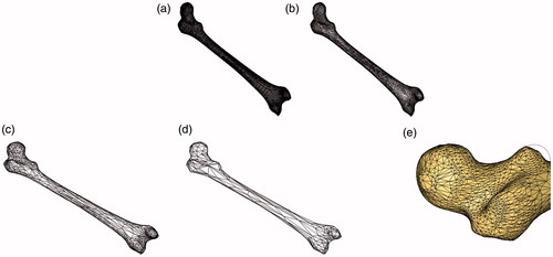
As seen in Figure 1, the algorithm of this study effectively produced multiresolutions implifications of the complex femur model, which maintained the details of the model and achieved the desired research goals. Because this study considered selective collapse, the triangles were dense in the large curvature area at the ends of the femur model and sparse in the small curvature area of the femoral shaft, as shown in Figure 1(c). Figure 1(d) maintains the model geometry features. However, the simplification is large, and some of the details are lost. As shown in Figure 1(e), the error accumulation was effectively avoided using the mean ranking of the collapse cost. Therefore, dense triangular tiles were retained in the highly curved region, and the detailed features of the model were maintained.

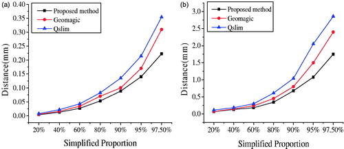
The model simplification algorithm QSlim 2.0 [20] and reverse engineering software Geomagic were also used to simplify the femur model, with simplifications of 20%, 40%, 60%, 80%, 90%, 95%, and 97.5%. The Metro tool [21] was used to calculate the mean distance and Hausdorff distance before and after the model was simplified.The results of the quantitative analysis of the geometric similarity of the model are shown in Figure 2. The simplification used in this study produced an observable advantage in relation to the geometric similarity. The mean distance represented the overall mean error of the model before and after simplification; the Hausdoff distance represented the maximum error. As shown in Figure 2, the slope of the curve increased and the simplified model was changed when the simplification was greater than 80%. A simplification of less than 80% produced a more appropriate model.

Figure 2. Mean and Hausdorff measurements of simplified model. (a) Mean distance of simplified model and (b) Hausdorffdistance of simplified model.

Results of hip mesh generation

The mesh-generation program developed in this research used Visual Studio 2010 on a Windows XP Microsoft system. The processor was an Intel (R), Xeon (R), E5606 running at 2.13 GHz, with a quad core. It used an 8GB DDR3 133 MHz memory and 1GBgraphic card.

In this work, the mesh-generation method was used for the simplified model of the femur and vastus lateralis muscle. The results are shown in Figures 3 and 4, respectively. Figure 3(a) shows a simplified model (25000 elements). Figure 3(b) shows a local-magnification graph of a partially simplified femur model. Figure 3(c) shows a portion of the femur surface mesh model, and Figure 3(d) shows an effect graph of the mesh refinement. Figure 3(e) shows a section view of the volume mesh. Figure 4(a) shows the surface-mesh model of the vastus lateralis muscle, and Figure 4(b) shows the section view of the vastus lateral volume mesh. Figures 3 and 4 show the following results. (1) Although the simplified model was a surface triangle model, there were long and narrow triangles, surface topology inconsistencies, rough tiles, etc. The low-quality surface mesh model was not an accurate input for generating a 3 D volume mesh, as shown in Figure 3(b). (2) Self-adaptive surface mesh generation occurred in the large curvature region in this study. The obtained element was approximately an equilateral triangle, which contained a smooth transition, adapted to the change in the curvature of the model, and maintained the model’s geometric features, as shown in Figures 3(d) and 4(a). (3) To effectively describe the shape of the curved surface, mesh refinement was performed using a feature constraint for the model, which adapted to the complex curved surface and maintained the geometric precision of the model, as shown in Figure 4(a) at two points. (4) During the volume mesh generation, the transition of the tetrahedral elements was smooth, as shown in Figures 3(e) and 4(b) at one point.

Figure 3. Mesh generation for femur. (a) Simplified model, (b) Partial model, (c) Surface mesh model, (d) Mesh refinement and (e) Body mesh model.

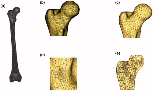
Figure 4. Mesh generation for vastus lateralis muscle. (a) Surface mesh model of vastus lateralis muscle and (b) Cutaway view of volume mesh of vastus lateralis.

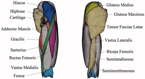
The hip consists of the hipbone, femur, hip muscle, and cartilage. Because of the limits imposed by the complexity of the human hip muscles and the accuracy of the 2 D image data, adjacent muscles and muscles with similar functions were combined during the modeling. Two human hip bones, 13 muscles, and one articular cartilage sample were modeled. Using the method proposed in this study, the hip model was simplified, and the mesh was generated. The results are shown in Figure 5. The method proposed in this study could be used to generate meshes for all the hip models. A model of the medial muscle of the femur and the rectus femoris muscle was not achieved using the direct automatic mesh generation of the HyperMesh because the boundary surface angle was too large. In this study, mesh generation was effective, and it was shown that the proposed method was adaptable to a complex model. In the assembly of the hip joint of the model, the mesh-generation result was similar to the original geometric model, which made the assembly model fit accurately. This was significant for the convergence of the finite-element analysis. Figure 5 shows that the mesh refinement of the large curvature area of the model was clear, and the transition was smooth.

Figure 5. Assembled model of hip.

Quality analysis of surface mesh generation

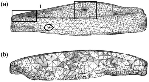
The surface triangular element was the basis for the tetrahedral-mesh generation. It not only determined the quality of the tetrahedral element, but also affected the computational accuracy of the biomechanics. Concurrently, the edges and surfaces of the original model should be approximated by the mesh, and the geometric precision of the model should be maintained before and after mesh generation. The mesh-generation method proposed in this study and the AFT algorithm in the Hypermesh software were used for the same model. Because this method proposed the addition of geometric self-adaptive local mesh refinement to the size control, the number of mesh elements was significantly greater than that of the existing software. The results are shown in Figure 6, where (A1) and (A2) are the mesh generation results obtained in this study, and (B1) and (B2) are the results of the existing software using the AFT algorithm.

Figure 6. Partial graphs of femur mesh. (A1) Mesh generation result of proposed method, (A2) Mesh generation result of proposed method, (B1) Mesh generation result of hypermesh software and (B2) Mesh generation result of hypermesh software.

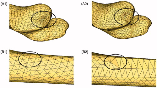
Figure 6(A1, A2) show that in the large curvature area of the model, the mesh-generation program produced a progressive mesh refinement. The transition between the elements was smooth, and the mesh in parts other than the large curvature area was sparse. The mesh generation results were uniform and contained an optimized element shape. Moreover, the geometric accuracy of the model was maintained. The quality of the surface triangular element of the femur model was analyzed using the smallest angle distribution of the triangles, and the results are listed in Table 1.

Table 1. Quality of surface triangular element.

					Angular distribution of the minimum angle (%)
Algorithm example	Global size (mm)	Number of triangles	Maximum angle (°)	Minimum angle (°)	0°–15°	15°–30°	30°–45°	45°–60°
Wang’s algorithm	5	8306	167.36	3.31	0.36	0.79	0.79	90.85
	6	6672	167.36	3.31	0.45	1.09	9.71	88.74
Existing software	5	6706	172.85	3.52	1.92	7.81	12.36	77.75
	4.5	8434	163.94	3.50	1.06	3.78	13.79	81.37
Simplified model	—	25000	169.92	3.31	32.55	30.51	24.75	12.18

The minimum angle in many triangles of the simplified model was between 0° and 30°. This type of triangle could not serve as an input for the tetrahedral mesh generation. Therefore, it was necessary to regenerate a high-quality surface mesh. When using Wang’s algorithm, most of the triangular surface elements had a minimum angle greater than 45°. Using triangle numbers with the optimal interval, Wang’s algorithm was superior to the existing software algorithms. Because the algorithm achieved mesh refinement in large curvature areas and contained more feature constraints, the total number of elements obtained by Wang’s algorithm was larger than that of the existing software. To make the verification more rigorous, the global size of the existing software was set to 4.5 mm when the global size of Wang’s algorithm was set to 5 mm. Concurrently, the overall numbers for the triangular grids obtained from the existing software and Wang’s algorithm were approximately equal. The mesh-generation results of this algorithm were 90.85% triangles with a minimum angular distribution between 45° and 60°. The mesh-generation results of the existing AFT software were 81.37% triangles with a minimum angular distribution between 45° and 60°. Table 1 shows that the uniformity of the surface mesh did not significantly change with the number of generated elements in this study. However, when using the AFT algorithm of the existing software for mesh generation, the uniformity of the surface mesh showed a greater change with an increase in the number of elements.

The mean and Hausdorff distances in the surface mesh-generation of the hip femur model were quantitatively analyzed using Metro. The results are listed in Table 2. The surface mesh results accurately approximated the original model and maintained the geometric accuracy of the model in this study.

Table 2. Mean and Haurdorff distances of surface mesh.

Algorithm	Global dimension (mm)	Number of nodes	Number of triangles	Mean	Hausdorff	Local refinement
Wang’s algorithm	5	4157	8306	0.098799	1.100910	Yes
	6	3390	6672	0.183113	1.545679	Yes
Exiting software	5	3357	6706	0.188196	6.445955	No
	4.5	4221	8434	0.144433	2.258001	No

Quality analysis of volume mesh generation

The quality of the volume mesh will directly affect the reliability, convergence, and efficiency of the finite-element calculations. The main objective of this study was to generate a high-quality and large-scale tetrahedral mesh hip model to meet the finite-element calculation requirements of biomechanics.

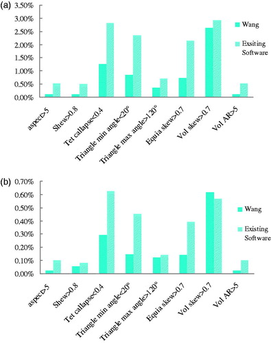
Using the check-elems tool of Hypermesh 13.0, the quality evaluation parameters of the mesh model were tested, and the quality of the volume mesh obtained from the proposed mesh-generation method was evaluated. The femoral and vastus lateralis mesh-generation results of this study were compared with the tetrahedral mesh-generation results of the existing software, and the results are shown in Figure 7. The eight groups of tetrahedral quality parameters were the aspect, skew, tet collapse, triangle min angle, triangle max angle, equia skew, volume skew, and volume AR. The results from Wang’s algorithm were more accurate than those of the existing software. The tetrahedral quality parameters of the vastus lateralis mesh generation using Wang’s algorithm were superior to the existing software results, except for the volume skew parameter.

Figure 7. Quality analysis results for volume-mesh generation. (a) Quality analysis of volume-mesh generation for femur and (b) Quality analysis of volume-mesh generation for vastus lateralis muscle.

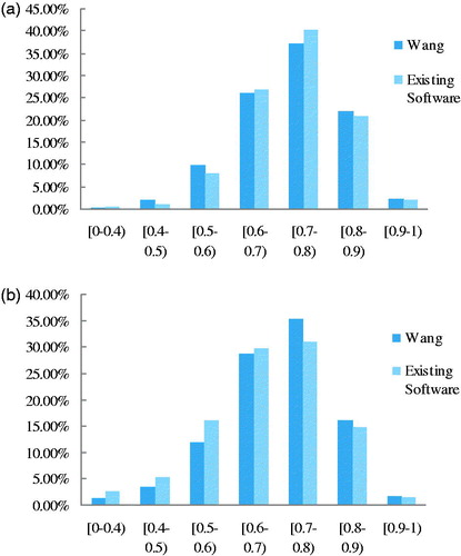
The distributions of the values for the tetrahedral element quality parameter tet collapse for the femoral and vastus lateralis models were analyzed, and the results are shown in Figure 8. If the tet collapse values were 0.6–0.8 for the general tetrahedral elements and 0.8–1 for the high-quality tetrahedral elements, the general tetrahedral elements obtained using Wang’s algorithm forthe femoral and vastuslateralis modelswere 64.14% and 63.32%, respectively. The average proportions from the existing software were 60.89% and 67.43% for the femoral and vastuslateralis models, respectively. The high-quality tetrahedral elements obtained using Wang’s algorithm for the femur and vastus lateralis muscle were 17.81% and 24.50%, respectively. The proportions from the existing software were 16.31% and 22.87% for the femoral and vastuslateralis models, respectively.

Figure 8. Tet collapse value distribution. (a) Tet collapse distribution of femur and (b) Tet collapse distribution of vastus lateralis muscle.

Table 3 presents the program running times needed by Wang’s algorithm to generate the meshes of the femur and vastus lateralis muscle. The number of volume mesh elements is expressed as Ne, and the total time formesh generation is expressed as T. The time sumsfor the feature recognition and establishment of the size control field are expressed as T_f. The times for the discretization of the curved boundary surface and triangle generation for the curved surface are expressed as T_l and T_s, respectively. The time for the mesh generation of the tetrahedral elements is T_t.

Table 3. Meshing efficiency analysis (unit: s).

Model	Ne	T	Tf	Tl	Ts	Tt
Femur	32392	207.61	18.16	18.86	84.12	86.47
Vastuslateralis	40424	214.29	16.39	17.12	83.94	96.84

The advantages of the proposed method included the ability to generate a mesh for a complex model. The mesh elements obtained were uniform and smooth, and retained the features of the original geometric model. The limitation of the proposed method was meshing time. We hope to do much work to improve the efficiency in the future.

Conclusions

In this work, considering the structural features of a human hip model, its geometric model was simplified using an edge-collapse algorithm based on QEM. Using the AFT and Delaunay algorithms, the surface mesh and tetrahedral mesh of the model were respectively generated according to the maximum global size. Through mesh size control, mesh refinement was automatically achieved for local, large curvature areas and additional feature areas. The program was completed in a Visual Studio 2010 environment using C++. Based on an analysis of the quality of the surface and volume mesh generation, it was concluded that the mesh generation method could be used to generate the mesh for a hip. The mesh elements obtained were uniform and smooth, and retained the features of the original geometric model.

Acknowledgements

This research was supported by National Natural Science Foundation of China [grant no. 61572159].

Disclosure statement

No potential conflict of interest was reported by the authors.

Additional information

Funding

This research was supported by National Natural Science Foundation of China [grant no. 61572159].

References

- Jamin C, Alliez P, Yvinec M, et al. CGAL mesh: a generic framework for Delaunay mesh generation. ACM Trans Math Softw. 2015;41:23.
- Romanoni A, Pollefeys M, Matteucci M. Automatic 3D reconstruction of manifold meshes via Delaunay triangulation and mesh sweeping. IEEE Winter Conf Appl Comput Vis. 2016;4:1–8.
- Chen X, Chen L, Shi M. A highly solid model boundary preserving method for large-scale parallel 3D Delaunay meshing on parallel computers. CAD. 2015;58:73–83.
- Chen J, Chen Z. Three‐dimensional superconvergent gradient recovery on tetrahedral meshes. Int J Numer Meth Eng. 2016;108:819–838.
- Pardue J, Chrisochoides N, Chernikov A. Parallel two-dimensional unstructured anisotropic Delaunay mesh generation for aerospace applications. Procedia Eng. 2015;4:1–5.
- Hoppe H. Progressive meshes. Proceedings of the 23rd Annual Conference On Computer Graphics and Interactive Techniques New Orleans, Association; 1996. p. 99–108.
- Low KL, Tan TS. Model simplification using vertex clustering. Proceedings of the Symposium on Interactive 3D Graphics; 1997. p. 75–81.
- Lounsbery M, DeRose TD, Warren J. Multiresolution analysis for surfaces of arbitrary topological type. ACM Trans Graph. 1997;16:34–73.
- Hinker P, Hansen C. Geometry optimization. Proceedings of the IEEE Visualization; 2003. p. 189–195.
- Yang WJ, Zhao JL, Fan L, et al. Automatic 3D mesh generation of composite solid propellant particles. Aeronaut Comput Tech. 2012;42:74–76.
- Lo SH. Volume discretization into tetrahedra-II 3D triangulation by advancing front approach. Comput Struct. 1991;39:501–511.
- Yan L. Efficient and reliable 3d constrained delaunay tetrahedral finite element mesh generation algorithm. Dalian (China): Dalian University of Technology; 2010. p. 6–11.
- Labelle F, Shewchuk JR. Fast tetrahedral meshes with good dihedral angles. ACM Trans Graphics. 2007;26:28–57.
- Zhang Y, Bajaj C, Sohn B-S. 3D finite element meshing from imaging data. Comput Methods Appl Mech Eng. 2005;194:5083–5100.
- Lu XL. Research on 3D model acquisition and mesh simplification algorithms. Cheng Du (China): Southwest Jiaotong University; 2012. p. 11–19.
- Yu WJ. Research on adaptive tetrahedral mesh generation algorithm based on geometric feature. Nan Jing (China): Nanjing Normal University; 2013. p. 30–31.
- Walton DJ, Meek DS. A triangular G1 patch from boundary curves. Comput Aided Design. 1996;28:113–123.
- Liang Y. Research on adaptive surface mesh generation. Hang Zhou (China): Zhejiang University; 2009. p. 75–76.
- Huang C. Three dimensional mesh generation method for boundary surface methods. Chang Sha (China): Hunan University; 2014. p. 56–80.
- Garland M. Qslim v2.0. 2004. Available from: http://mgarlang.org/software/qslim20.html.
- Cignoni P, Rocchini C, Scopigno R. Measuring error on simplified surfaces. Comput Graph Forum. 1998;17:167–174.