Optimal distance of multi-plane sensor in three-dimensional electrical impedance tomography

Abstract

Electrical impedance tomography (EIT) is a visual imaging technique for obtaining the conductivity and permittivity distributions in the domain of interest. As an advanced technique, EIT has the potential to be a valuable tool for continuously bedside monitoring of pulmonary function. The EIT applications in any three-dimensional (3 D) field are very limited to the 3 D effects, i.e. the distribution of electric field spreads far beyond the electrode plane. The 3 D effects can result in measurement errors and image distortion. An important way to overcome the 3 D effect is to use the multiple groups of sensors. The aim of this paper is to find the best space resolution of EIT image over various electrode planes and select an optimal plane spacing in a 3 D EIT sensor, and provide guidance for 3 D EIT electrodes placement in monitoring lung function. In simulation and experiment, several typical conductivity distribution models, such as one rod (central, midway and edge), two rods and three rods, are set at different plane spacings between the two electrode planes. A Tikhonov regularization algorithm is utilized for reconstructing the images; the relative error and the correlation coefficient are utilized for evaluating the image quality. Based on numerical simulation and experimental results, the image performance at different spacing conditions is evaluated. The results demonstrate that there exists an optimal plane spacing between the two electrode planes for 3 D EIT sensor. And then the selection of the optimal plane spacing between the electrode planes is suggested for the electrodes placement of multi-plane EIT sensor.

Keywords:

• Electrical impedance tomography
• pulmonary function monitoring
• spacing optimization
• three-dimensional effects
• multi-plane sensor

1. Introduction

Electrical impedance tomography (EIT) is one kind of functional tomography techniques which are visual imaging technique. In EIT imaging, sinusoidal electric currents are applied to the target of interest using electrodes, and the resulting voltages measured from boundary electrodes are carried out to obtain information on the conductivity and permittivity distributions within the target [1–3]. Compared to other tomography techniques, such as chest x-ray (CXR) and computed tomography (CT), EIT has the advantages of high speed, low cost, portability, non-invasion and non-radiation, which make it a promising monitoring technique with applications in many fields, such as industry processing imaging and medical diagnosis [4,5].

The most common medical application of EIT is thorax tomography. As a novel monitoring technique of human thorax, EIT provides a means of analyzing ventilation distribution in the lungs, where the data is continuously displayed as images, wave-forms, and parameters. Based on the conductivity changes of contrasting air and blood flow in lungs, the bio-electrical properties of pulmonary tissue can be imaged by EIT. In addition, EIT can be used for continuously bedside monitoring the condition of patients suffering from acute respiratory distress syndrome (ARDS) in intensive care units (ICU) [6–8].

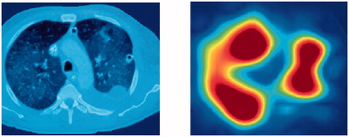
Currently, CXR and CT scans are the only universally available medical imaging techniques which can obtain regional information of the lungs [9]. As shown in Figure 1, functional EIT image and CT scan come from a patient with a pleural effusion after rupture of the diaphragm, resulting in a significantly reduced ventilation of the lower left lung. The red color represents regions with the highest volume changes, the non-ventilated regions are displayed in deep blue. While the CT scan provides images of morphologic structures with a high spatial resolution, EIT provides functional images with a relative low spatial, but very high temporal resolution. This means that the clinician can follow the response of the lung to some therapeutic measures on a respiratory basis after the assessment of radiological images. Thus, EIT could be used as a complementary tool to radiological techniques and realize the monitoring to the patient’s lung function [10–12].

Figure 1. CT scan (left) and functional EIT image (right) from a patient.

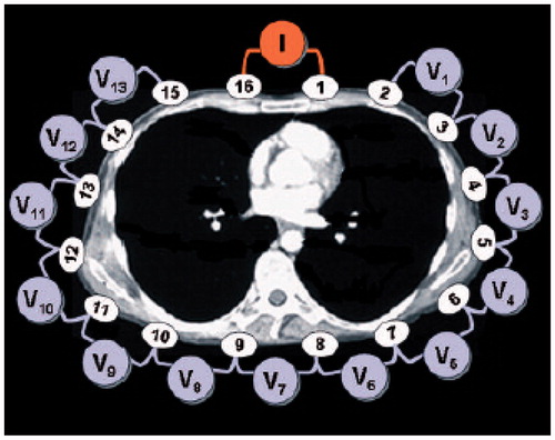
To monitor pulmonary impedance changes, as shown in Figure 2, electrodes have to be placed around the patient’s chest wall, tiny electric currents are applied to the body through one electrode pair and the resulting voltages are measured simultaneously at other electrode pairs. These voltages change in relation to the amount of air and blood flow present in the patient’s chest [13].

Figure 2. Monitoring the changes of thoracic impedance.

For clinical use, the excitation signals are usually selected as sinusoidal waveforms whose amplitude and frequency ranges are limited by the IEC60601-1-1 standard for patient safety. In order to ensure the patient safety, the order of magnitude of electric current applied to the body is mA level. According to the IEC 60601-1-1 standard, the relationship between the maximum amplitude and frequency of excitation current can be calculated by 0.1 × f mA, where f is the excitation frequency in kHz, in addition the amplitude of excitation current should be also less than 10 mA. For most EIT system, the frequencies of excitation current are generally ranging from several kHz to 1 MHz. An EIT system with the frequency ranging from 10 kHz to 10 MHz has been developed by Halter R J, et al. [14]. In this paper, the EIT system used in experiment is developed by Tianjin University [15], in which the amplitude of excitation current is less than 5 mA, and the frequency range is from 10 kHz to 1 MHz.

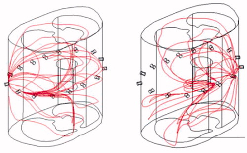
However, there exist many factors which limit the extended application of the EIT technique. Firstly, in electrical impedance tomography, the electric field distribution of the sensing field will change with the distribution of material conductivity in the field, which nature is so-called the “soft-field” effect. This property enhances the difficulty of image reconstruction and explanation, so a prior knowledge of the medium distribution inside sensing field is often needed [15–17]. Secondly, in two-dimensional (2 D) EIT, an array of electrodes is attached around human thorax and the images are reconstructed based on the assumption that the injected electric currents are confined to the 2 D electrode plane. However, the sensing field of the EIT system is an inherently three-dimensional (3 D) electric field distribution, where the injected electric currents are not constrained to the plane within the excitation electrodes, but spread out in three dimensions when electric currents pass through the chest [18–20], as shown in Figure 3.

Figure 3. Current density distributions in 3 D condition.

Since the sensing field of real EIT sensor is distributed in a 3 D space, the data obtained from the EIT system reflects the conductivity distribution in a certain space instead of a plane. Therefore, it is difficult to guarantee the accuracy and clarity of a 2 D image reconstructed from the 3 D data [16–18]. For the reasons of actual 3 D electric field distribution and physical field, many research groups have been investigated the 3 D EIT technique [19–22]. It could be used for depicting more truly physiological information of interest and properly estimating the sizes of thoracic organs than 2 D EIT.

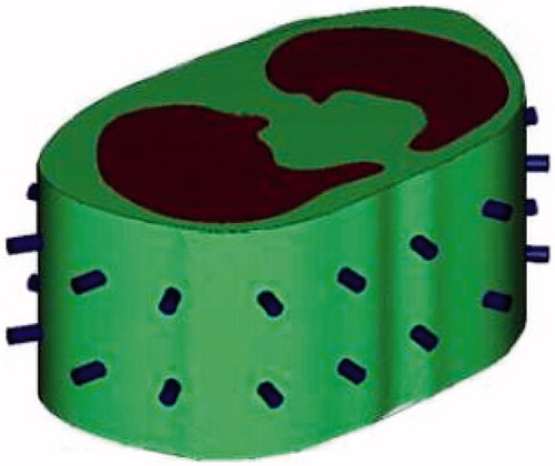
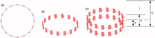
Most 2 D thoracic EIT uses a single plane of electrodes on the chest [20], as shown in Figure 2, but for 3 D EIT, two or more electrode planes are needed [21], as shown in Figure 4. Though multi-plane EIT sensors are often used for 3 D image reconstruction [22–23], little literature has investigated spacing optimization of multi-plane sensor for 3 D EIT and its effects on the electric field distribution and imaging accuracy. In this paper, a two-plane EIT sensor is designed where each plane consists of 16 electrodes, and the plane spacing between the two electrode planes is adjustable by adding or reducing the number of the Perspex annulus. The aim of this paper is to find the best spacing resolution of EIT image over various electrode planes and select an optimal plane spacing in a 3 D EIT sensor, and thus provide guidance for 3 D EIT electrodes placement in monitoring lung function.

Figure 4. Two-plane sensor array in 3 D model.

2. Mathematical model of EIT

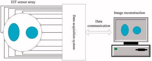
EIT aims to estimate the interior conductivity distribution of an unknown object from a set of boundary measurements [1–3]. To realize this goal, a set of electrodes are attached around the body surface. And then the boundary voltages, caused by the conductivity distribution variation in the sensing filed, are obtained by the data acquisition system. Finally, the internal conductivity distributions of the measured object are reconstructed through the certain reconstruction algorithm. A typical EIT system is illustrated in Figure 5. It consists of three main parts: sensor array, data acquisition system and image reconstruction system.

Figure 5. EIT system with 16-electrode sensor.

The mathematical relation between the measured boundary voltages and the conductivity distribution can be expressed as [24] (1) where σ is the electric conductivity inside the sensing field, u is the measured boundary voltages. The linearized and discretized form of Equation (1)(1) can be represented as (2) where b is the variations of the measured boundary voltages, A is the Jacobin matrix and x is the electric conductivity distributions. The Jacobin matrix A is calculated based on Geselowitz’s sensitivity theorem [25].

3. Image reconstruction algorithm and EIT sensor

3.1. Tikhonov regularization method

The Tikhonov regularization is an effective method to deal with the ill-posed inverse problem, which has been used for recent decades in the image reconstruction of electrical impedance tomography. Essentially, the method is to convert solving the inverse problem of Equation (2)(2) into an optimization problem (3) where λ is a positive parameter, which is used to adjust the weight between the two parts of the function, L is one kind of liner operator, which usually represents the first or second derivative operator. If L is the identity matrix, i.e., the zero-order derivative operator, the Tikhonov problem Equation (3)(3) turns out to be a standard form as (4)

As a result, under a certain regularization parameter λ, the regularized solution x is then calculated by the following normal equation (5)

3.2. Principle of measuring spatial resolution

The EIT imaging process follows the general Maxwell equation [26], whose general physical model can be written as (6) where f(σ) is boundary condition. In a cylindrical coordinate, ∇²φ can be rewritten as (7)

We focus on find any two-dimensional field and thus assume there is unchangeable in the θ-axis direction, thus ∂²φ/∂z²=0, and further assume the solution has the following forms as φ = f(r)g(z), we get (8)

The first item in Equation (8)(8) contains only the unique variable r, and second item is variable z, thus they must equal to a constant that is denoted as k², that is (9)

Equation (9)(9) is two ordinary equations and their solutions can be directly obtained. After substituting their solutions into φ = f(r)g(z), we obtain (10) when T = jτ and τ is a real constant, Equation (10)(10) is turned to (11) where I₀(τr) and K₀(τr) are zero-order first-type and second-type Bessel function, respectively.

These parameters in Equations (10)(10) and (11)(11) are unknown, but can be determined by prior information once the tested model is fixed. For the three-dimensional case, we compute the voltage distribution in various two-dimensional planes, and thus find the optimal distance between any pair of planes by Equations (10)(10) and (11)(11) in together.

3.3. Simulation models for EIT sensor

All the simulations are carried out in a COMSOL 3.5a with MATLAB (R2009b) environment running in an Intel Core2 Duo CPU of 2.00 GHz. The finite element method (FEM) and adjacent excitation/measurement scheme are exploited for solving the forward problem of the EIT system.

The influence of contact impedance between electrode and skin should be considered when an EIT sensor is designed. A simulation research on the influence of electrode width using the coercive equipotential node FEM model was carried out by Wang. et al. [27–28], and showed that the best effect was obtained when the overlay rate of electrodes was 57.1%. Reference [29] discussed the influence of electrode size on reconstruction. It has been shown that increasing the electrode size is equivalent to reducing the maximal value of the potential gradient and to introducing the averaging effect of a voltage measurement electrode. As a result, the variance of Jacobian’s element values is reduced. From the perspective of resolution coverage area, the electrode size should be large enough; from the perspective of resolution, the electrode size should also be smaller enough; in addition, considering the influence of contact impedance and the anti-noise capacity, the ratio of electrode width to model perimeter is set to 0.32. Based on the determined two-plane EIT sensor, this paper aims to study the plane spacing optimization and select an optimum spacing.

In this paper, a two-plane EIT sensor is designed where each plane consists of 16 electrodes, and the spacing between the two electrode planes is adjustable. The real two-plane EIT sensor has seven kinds of spacing are used for experimental verification. In comparison, a 2 D EIT sensor model and a 3 D single-plane EIT sensor model are also established.

The conductivity distribution within the object is calculated by solving the inverse problem using a model of the physical set-up such as a finite element mesh (FEM) model based on the experimental data of the excitation current signals, the measured voltage signals and the predetermined shape of the object. The model layers or elements of different conductivity (body tissues) have not been considered in simulation. There are three reasons as follows. Firstly, the model layers or elements of different conductivity (body tissues) in simulation are not verified reasonably by experiment, and without the qualifications, the real human experiments are not permitted. Secondly, in this paper the plane spacing between the upper and lower electrode plane is little changed, so the thorax model can be simplified without considering the different conductivity. Finally, three-plane or more complex modeling introduced by Grychtol B [21]. dramatically increases the complexity of the hardware system and the dimension of sensitivity coefficient matrix. Besides, the algorithm implementation and image reconstruction are very time-consuming. Low-frequency simplifications of Maxwell’s equations are normally used, though a full solution has been investigated and found to be advisable for excitations at or above 1 MHz [26]. Therefore, a simplified thorax model attached two plane electrodes is more actual than the complex model in simulation and experiment.

Three EIT sensor models are used in simulations as shown in Figure 6. Figure 6(a,b) show a 2 D EIT sensor model and a 3 D EIT sensor model, respectively, which are utilized as comparisons for the 3 D two-plane EIT sensor model. For the Figure 2(c), seven kinds of spacings between the two electrode planes are used in simulation. S1, S2 … S7 are the symbols of the seven spacings, respectively, which are gradually increasing. The upper and lower electrode planes keep parallel. Besides, no rotation is guaranteed between the two electrode planes. Electric currents are applied to the electrode pairs of the upper and lower planes simultaneously. The boundary voltages measured from the two electrode planes are used to image reconstruction, respectively. Same operations are performed at different plane spacings.

Figure 6. 2 D and 3 D EIT sensor models. (a) 2 D EIT sensor model (b) 3 D single-plane EIT (c) 3 D two-plane EIT sensor model sensor model.

Note that the parameters of two-plane EIT sensor are shown as follows:

• Number of electrodes per electrode plane: 16

• Material of the tube: Perspex

• Inner diameter of the tube: 16 cm

• Thickness of the tube wall: 1.0 cm

• Material of electrode: Steel

• Size of electrode: 2.0 cm × 1.0 cm × 0.1 cm

• Spacing between the two electrode planes (adjustable): 1.5, 2.5, 3.5, 4.5, 5.5, 6.5 and 7.5cm

• Height of the tube (adjustable): 19.5, 20.5, 21.5, 22.5, 23.5, 24.5 and 25.5 cm.

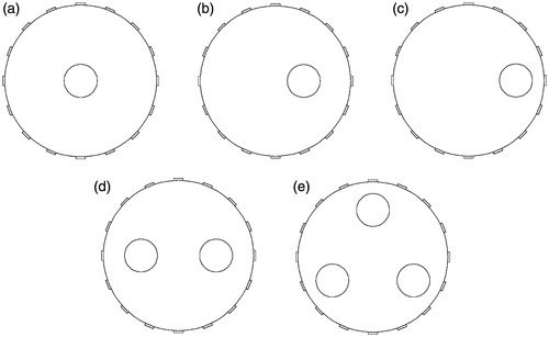
As shown in Figure 7, five typical conductivity distribution models, including one object (central, midway and edge), two objects and three objects, are set for different EIT sensor models. Note that saline with conductivity of 0.02 S/m and the rod with conductivity of 1.0 × 10⁻⁶S/m are used as background medium and the inclusion respectively inside the EIT sensor in all the following 2 D and 3 D simulations, and the Perspex rod with a diameter of 3.5 cm is selected as the measured object.

Figure 7. Cross-section view with object distribution. (a) One rod at centre (b) One rod at midway (c) One rod at edge (d) Two rods (e) Three rods.

3.4 Simulation results

To quantitatively evaluate the quality of the reconstructed image, the two indexes named relative error and correlation coefficient are utilized, and they can be calculated as (12) (13) where RE is the relative error, CC is the correlation coefficient, x is the real conductivity distribution, x^ is the reconstructed conductivity distribution inside the EIT sensor plane, x_i and x^_i are i-th elements of x and x¯, respectively, and x^¯ are the mean values of x and x^, respectively.

In this paper, the boundary voltages obtained from the lower electrode plane of the two-plane EIT sensor are used in image reconstruction. A Tikhonov regularization method is selected as the image reconstruction algorithm. Note that for the 2 D simulation, the regularization parameters are set as, 0.0001, 0.0001, 0.0001, 0.03 and 0.2 respectively for the five models, and for the 3 D single-plane EIT sensor and 3 D two-plane EIT sensor, the regularization parameters are set as, 0.00001, 0.00001, 0.01, 0.01 and 0.02 respectively for the five models. For the 3 D two-plane EIT sensor, each plane possesses 16 electrodes. Correspondingly, the number of the measured boundary voltages per plane is 208. For convenient comparison with the set conductivity distribution, all of the reconstructed images are normalized to the range from 0 to 1.

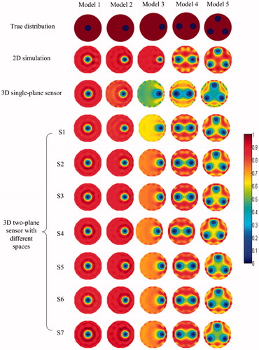
The simulation results of image reconstruction for the five models are shown in Figure 8. The first row of Figure 8 lists the true distributions of the five simulation models, the second row and the third row give the results of image reconstruction for 2 D simulation and 3 D single-plane EIT sensor, respectively, which are chosen to be the comparisons for the 3 D two-plane EIT sensor, the forth row to the last row show the results of 3 D two-plane EIT sensor with different spacings between the upper and lower electrode planes, respectively.

Figure 8. The simulation results of image reconstruction for five models.

The correlation coefficient and relative error are selected as the two quantitative criteria for evaluating the performance of the reconstructed images. Tables 1 and 2 show the data of correlation coefficient and relative error of the five models in simulation, respectively. To show more clearly the effect of the 3 D two- plane EIT sensor with different spacings, the data in Tables 1 and 2 are displayed in Figures 9 and 10, respectively.

Figure 9. The correlation coefficient of the five models with different spacings for the 3 D two-plane EIT sensor.

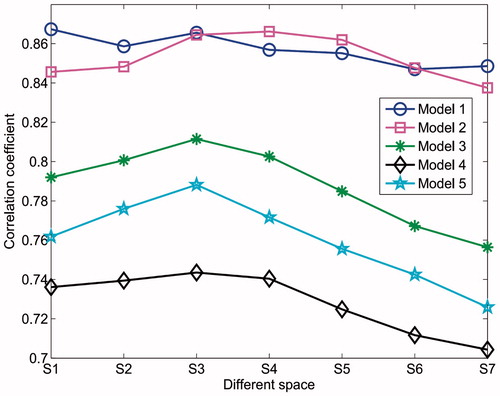
Figure 10. The relative error of the five models with different spacings for the 3 D two-plane EIT sensor.

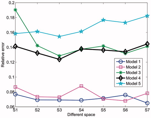
Table 1. The correlation coefficient of the five models in simulation.

	Model 1	Model 2	Model 3	Model 4	Model 5
2D simulation	0.8637	0.8927	0.9115	0.7741	0.8251
3D single-plane sensor	0.8450	0.7848	0.6706	0.6541	0.6758
3D two-plane sensor with different spacings
S1	0.8674	0.8457	0.7920	0.7361	0.7618
S2	0.8587	0.8483	0.8007	0.7394	0.7760
S3	0.8656	0.8645	0.8115	0.7435	0.7882
S4	0.8569	0.8662	0.8026	0.7404	0.7716
S5	0.8552	0.8620	0.7849	0.7248	0.7556
S6	0.8470	0.8477	0.7672	0.7117	0.7425
S7	0.8486	0.8376	0.7564	0.7043	0.7259

Table 2. The relative error of the five models in simulation.

	Model 1	Model 2	Model 3	Model 4	Model 5
2D simulation	0.0657	0.0585	0.0604	0.1317	0.1232
3D single-plane sensor	0.0694	0.1031	0.2449	0.1956	0.2136
3D two-plane sensor with different spacings
S1	0.0768	0.0866	0.1904	0.1414	0.1584
S2	0.0693	0.0735	0.1423	0.1323	0.1612
S3	0.0692	0.0729	0.1285	0.1238	0.1545
S4	0.0688	0.0880	0.1374	0.1378	0.1613
S5	0.0715	0.0706	0.1418	0.1363	0.1767
S6	0.0759	0.0681	0.1317	0.1341	0.1731
S7	0.0650	0.0782	0.0604	0.1446	0.1823

Figures 9 and 10 show the correlation coefficient and the relative error of the five models with different spacings for the 3 D two-plane EIT sensor. When the plane spacing between the two electrode planes is S3, i.e. the spacing between the upper and lower electrode planes is 3.5 cm, the correlation coefficients of the five models reach the peak values, i.e. 0.8656, 0.8645, 0.8115, 0.7435 and 0.7882 respectively, and the relative errors reach the lowest values, i.e. 0.0692, 0.0729, 0.1285, 0.1238 and 0.1545 respectively. This demonstrates that the S3 (3.5 cm) is the optimal plane spacing for the five models in 3 D two-plane EIT sensor.

As can be seen from the simulation results of models 1 and 2, there are no significant differences between 2 D and 3 D conditions of EIT sensor, which lies in non-sensitive to central field. Thus, the variation of plane spacing for two-plane EIT sensor has little influence on the image reconstruction of models 1 and 2. For the models 3, 4 and 5, there are obvious distinctions on image reconstruction results between 2 D and 3 D conditions of EIT sensor, and the results of image reconstruction are changing with the plane spacing of 3 D EIT senor, especially, when the spacing reaches a certain position (S3 in this paper), the reconstructed images achieve optimal performance.

4. Experimental results and discussion

4.1. Experiment setup

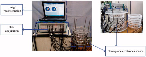
To validate the findings with the two-plane EIT sensor, an EIT system with 32-electrode channels developed by Tianjin University [15] is used in static experiments. The experimental setup is shown in Figure 11. Correspondingly, a two-plane EIT sensor is designed where each plane consists of 16 electrodes, and the spacing between the two electrode planes is adjustable. Adjacent excitation/measurement scheme is exploited in experiment. The electric current is injected between one pair of neighboring electrodes, and the differential potentials between all remaining pairs of adjacent electrodes are measured. The frequency of alternating current in the EIT system is 100 kHz. Perspex rod with a diameter of 3.5 cm is positioned in water tank during the experiments. Saline with the conductivity of 0.02 S/m is selected as the background medium. Five experimental models are created using Perspex rods as same as the simulation models.

Figure 11. Experimental setup.

The real EIT sensor has seven kinds of spacings are used for experimental verification. The spacing between the two electrode planes can be adjustable through adding or reducing the number of the Perspex annulus. At each spacing condition, the boundary voltages obtained from the lower plane electrodes for the five models are collected through the EIT system. To illustrate the difference between two-plane and single-plane EIT sensor, a set of experiments for the five models with single-plane EIT sensor is also set up as a comparison. A Tikhonov regularization method is also selected as the image reconstruction algorithm. Note that for the 3 D single-plane EIT sensor and 3 D two-plane EIT sensor, the regularization parameters are set as, 0.00001, 0.00001, 0.01, 0.01 and 0.02 respectively for the five models.

4.2. Experimental results and analysis

The results of image reconstruction using the experimental data of the five models are listed in Figure 12. The corresponding quantitative criteria, i.e. correlation coefficient and relative error, are listed in Tables 3 and 4, respectively. The correlation coefficient and relative error of the five models for two-plane EIT sensor at different plane spacings are displayed in Figures 13 and 14.

Figure 12. The experimental results of image reconstruction for five models.

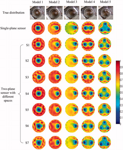
Figure 13. The correlation coefficient of the five models with different spacings for the two-plane EIT sensor.

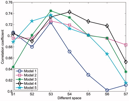
Figure 14. The relative error of the five models with different spacings for the two-plane EIT sensor.

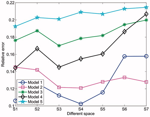
Table 3. The correlation coefficient of the five models in real experiment.

	Model 1	Model 2	Model 3	Model 4	Model 5
3D single-plane sensor	0.6532	0.7045	0.5612	0.6410	0.6130
3D two-plane sensor with different spacings
S1	0.7058	0.6956	0.6438	0.7041	0.6890
S2	0.6801	0.6958	0.7010	0.6903	0.7264
S3	0.7239	0.7266	0.7448	0.7338	0.7371
S4	0.6715	0.7192	0.7328	0.7427	0.7129
S5	0.6298	0.7011	0.7005	0.7257	0.7013
S6	0.6021	0.6953	0.6959	0.7178	0.6672
S7	0.6117	0.6837	0.6352	0.6530	0.6153

Table 4. The relative error of the five models in real experiment.

	Model 1	Model 2	Model 3	Model 4	Model 5
3D single-plane sensor	0.1124	0.1579	0.2011	0.1672	0.2113
3D two-plane sensor with different spacings
S1	0.1061	0.1451	0.1762	0.1442	0.1925
S2	0.1264	0.1420	0.1874	0.1667	0.2027
S3	0.1122	0.1217	0.1701	0.1451	0.2010
S4	0.1024	0.1209	0.1785	0.1548	0.2090
S5	0.1158	0.1281	0.1819	0.1605	0.2068
S6	0.1577	0.1332	0.1945	0.1864	0.2129
S7	0.1578	0.1280	0.1998	0.2068	0.2146

As shown in Table 3, for the model 1, the correlation coefficient of the image reconstructed from the 3 D single-plane sensor, i.e. 0.6532, is smaller than that from the 3 D two-plane sensor for the first four plane spacings, i.e. S1 to S4; the results obtained from S5 to S7 are contrary. For the model 2, the correlation coefficient of the image reconstructed from the 3 D single-plane sensor i.e. 0.7045, is larger than that from the 3 D two-plane sensor for the first and last two plane spacings, i.e. S1, S2, S6 and S7; the results obtained from S3 to S5 are contrary. For the models 3, 4 and 5, the correlation coefficients of the images reconstructed from the 3 D two-plane sensor are all larger than that from the corresponding 3 D single-plane sensor, i.e. 0.5612, 0.6410 and 0.6130, respectively.

As shown in Table 4, for the model 1, the relative error of the image reconstructed from the 3 D single-plane sensor, i.e. 0.1124, is larger than that from the 3 D two-plane sensor for the two plane spacings, i.e. S1 and S3; the results obtained from the other five plane spacings are contrary. For the models 2 and 3, the relative errors of the images reconstructed from the 3 D two-plane sensor are all smaller than that from the corresponding 3 D single-plane sensor, i.e. 0.1579 and 2011, respectively. For the model 4, the relative error of the image reconstructed from the 3 D single-plane sensor, i.e. 0.1672, is larger than that from the 3 D two-plane sensor for the four plane spacings, i.e. S1 and S3 to S5; the results obtained from the other three plane spacings are contrary. For the model 5, the relative error of the image reconstructed from the 3 D single-plane sensor, i.e. 0.2113, is larger than that from the 3 D two-plane sensor for the first five plane spacings, i.e. S1 to S5; the results obtained from the other two plane spacings are contrary.

Figure 13 shows, for all models except for model 4, the correlation coefficients reach the peak values, i.e. 0.7269, 0.7226, 0.7448 and 0.7371, respectively at the plane spacing of S3 (3.5 cm); for the model 4, though the S3 is the not optimal point, the correlation coefficient (0.7338) at this point is very closely to the peak value (0.7427) at the plane spacing of S4.

Figure 14 shows, for all models except for model 1, the relative errors reach the lowest values, i.e. 0.1219, 0.1701, 0.1451 and 0.2010, respectively at the plane spacing of S3; for model 1, the relative error (0.1122) at the point of S3 is very closely to the lowest value (0.1024) at the plane spacing of S4. In addition, for the five models, the correlation coefficients and relative errors calculated from the 3 D two-plane sensor at first few plane spacings are better than the corresponding values calculated from 3 D single-plane sensor.

An empirical compensation relationship between the two electrode planes can be given as following equation (14) where V_m is the measured vector of potential differences after compensation, V_b and V_t are the measured vectors of potential differences from the bottom and top electrode planes, respectively, and k is the weighting factor, which is a small positive scalar and initially determined based on trial-and-error for the optimum result.

The above experimental results confirm that the previous simulation results are valid. It illustrates that the 3 D two-plane EIT sensor can improve the accuracy and stability of reconstructed images. It also shows that the image quality can achieve optimal performance by properly adjusting the plane spacing between the upper and lower electrode planes. However, due to the insensitivity to central region distribution for electrical impedance tomography, it has no obvious improvement on the image quality for the central object by adjusting the plane spacing of 3 D two-plane EIT sensor. In addition, the simulation and experimental results also demonstrate that using the multi-plane EIT sensor can achieve better image reconstruction performance compared to the single-plane EIT sensor, since the placement of multi-plane electrodes is closer to real 3 D electric field distribution, besides using the multi-plane EIT sensor can improve the 3 D effect of electric field distribution for EIT system.

Conclusions

In this paper, a two-plane EIT sensor is designed where each plane consists of 16 electrodes, and the plane spacing between the two electrode planes can be adjusted through adding or reducing the number of the Perspex annulus. Several typical conductivity distribution models, including one rod (central, midway and edge inside the pipeline), two rods and three rods, are set as the simulation and experiment models. This study investigates the image performance at different plane spacings between two electrode planes of the two-plane EIT sensor and its effects on the electric field distribution and imaging accuracy in 3 D EIT sensor.

The results of this study can provide guidance for 3 D EIT electrodes placement in monitoring lung function. Although all the results are illustrated in this paper based on the lower plane electrodes of the two-plane EIT sensor, the same results can also be obtained from the upper one. It is suggested that the image reconstruction results are affected by the plane spacing between the upper and lower electrode planes of the two-plane EIT sensor. Simulation and experiment results demonstrate the quality of image reconstruction can achieve optimal by properly adjusting the plane spacing between two electrode planes. This work also provides a foundation research on 3 D electrical impedance imaging.

Future work will investigate the multi-plane EIT sensor, because it is beneficial for 3 D image reconstruction and pulmonary function monitoring. In addition, future work will also investigate the compensation relationship between the electrode planes, and its effects on 3 D reconstruction.

Disclosure statement

No potential conflict of interest was reported by the authors.

Additional information

Funding

The authors would like to thank the financial supports from the National Natural Science Foundation of China (No. 61573251).

References

- Cheney M, Isaacson D, Newell JC. Electrical impedance tomography. SIAM Rev. 1999;41:85–101.
- Nguyen DT, Jin C, Thiagalingam A, et al. A review on electrical impedance tomography for pulmonary perfusion imaging. Physiol Meas. 2012;33:695–706.
- York T. Status of electrical tomography in industrial applications. J Electron Imaging. 2001;10:608–619.
- Tapp HS, Peyton AJ, Kemsley EK, et al. Chemical engineering applications of electrical process tomography. Sens Actuators B Chem. 2003;92:17–24.
- Bodenstein M, David M, Markstaller K. Principles of electrical impedance tomography and its clinical application. Crit Care Med. 2009;37:713–724.
- Bikker IG, Leonhardt S, Bakker J, et al. Lung volume calculated from electrical impedance tomography in ICU patients at different PEEP levels. Intensive Care Med. 2009;35:1362–1367.
- Pikkemaat R, Lundin S, Stenqvist O, et al. Recent advances in and limitations of cardiac output monitoring by means of electrical impedance tomography. Anesth Analg. 2014;119:76–83.
- Ambrisko TD, Schramel JP, Adler A, et al. Assessment of distribution of ventilation by electrical impedance tomography in standing horses. Physiol Meas. 2015;37:175–186.
- Adler A, Amato MB, Arnold JH, et al. Whither lung EIT: Where are we, where do we want to go and what do we need to get there? Physiol Meas. 2012;33:679–694.
- Meier T, Leibecke T, Eckmann C, et al. Electrical impedance tomography: changes in distribution of pulmonary ventilation during laparoscopic surgery in a porcine model. Langenbecks Arch Surg. 2006;391:383–389.
- Zhang J, Patterson RP. EIT images of ventilation: what contributes to the resistivity changes? Physiol Meas. 2005;26:S81–S92.
- Adler A, Grychtol B, Bayford R. Why is EIT so hard, and what are we doing about it? Physiol Meas. 2015;36:1067–1073.
- Polydorides N, McCann H. Electrode configurations for improved spatial resolution in electrical impedance tomography. Meas Sci Technol. 2002;13:1862–1870.
- Sun J, Yang W. Fringe effect of electrical capacitance and resistance tomography sensors. Meas Sci Technol. 2013;24:1–15.
- Cui ZQ, Wang HX, Tang L, et al. A specific data acquisition scheme for electrical tomography. Paper presented at: I2MTC-IEEE International Instrumentation and Measurement Technology Conference; 2008 May 12–15; Victoria, Vancouver Island, Canada.
- Wang M. Three-dimensional effects in electrical impedance tomography. Paper presented at: 1st World Congress on Industrial Process Tomography; 1999 Apr 14–17; Buxton, Greater Manchester, UK.
- Yan H, Shao FQ, Xu H, et al. Three-dimensional analysis of electrical capacitance tomography sensing fields. Meas Sci Technol. 1999;10:717–725.
- Metherall P, Barber DC, Smallwood RH, et al. Three-dimensional electrical impedance tomography. Nature. 1996;380:1–6.
- Dehghani H, Soni N, Halter R, et al. Excitation patterns in three-dimensional electrical impedance tomography. Physiol Meas. 2005;26:S185–S197.
- Fan WR, Wang HX. 3D modelling of the human thorax for ventilation distribution measured through electrical impedance tomography. Meas Sci Technol. 2010;21:115801.
- Graham BM, Adler A. Electrode placement configurations for 3D EIT. Physiol Meas. 2007;28:S29–S44.
- Grychtol B, Müller B, Adler A. 3D EIT image reconstruction with GREIT. Physiol Meas. 2016;37:785–800.
- Mao M, Ye J, Wang H, et al. Evaluation of excitation strategy with multi-plane electrical capacitance tomography sensor. Meas Sci Technol. 2016;27:114008.
- Vauhkonen M. Electrical impedance tomography andprior information [dissertation]. Joensuu: University of Kuopio; 1997.
- Geselowitz DB. An application of electrocardiographic lead theory to impedance plethysmography. IEEE Trans Biomed Eng. 1971;18:38–41.
- Soni NK, Paulsen KD, Dehghani H, et al. Finite element implementation of Maxwell′s equations for image reconstruction in electrical impedance tomography. IEEE Trans Med Imaging. 2006;25:55–61.
- Wang H, Wang C, Yin W. Optimum design of the structure of the electrode for a medical EIT system. Meas Sci Technol. 2001;12:1020.
- Wang C, Wang H. Optimizing design of electrode construction in medical electrical impedance tomography system. J Fourth Mil Med Univ. 2001;22:78–80.
- Yan W, Hong S, Chaoshi R. Optimum design of electrode structure and parameters in electrical impedance tomography. Physiol Meas. 2006;27:291–306.