Three-dimensional analysis of acetabular orientation using a semi-automated algorithm

Abstract

Understanding the morphology of the acetabulum is necessary for preoperative evaluation in hip surgery. The purpose of this study was to (1) establish a novel method for measuring three-dimensional (3D) acetabular orientation, (2) quantify the reliability of this method, and (3) describe relevant characteristics of three-dimensional (3D) acetabular orientation among normal Asian subjects. Computed tomography (CT) scans of the pelvis that had been performed for suspected non-musculoskeletal conditions were obtained from 200 subjects (60 males, 140 females). A novel method was developed to measure 3D acetabular orientation with a semi-automatically determined pelvic coordinate system based on the anterior pelvic plane (APP). To quantify the robustness of our method, we analyzed the results obtained from 20 patients at different times and with different raters and pelvic poses in the same CT volume. To determine morphological differences of the acetabulum by age and sex, we analyzed the parameters of 200 CT volumes. Each intraclass correlation coefficient (ICC) values for intra- and inter-observer reliability were over 0.975 and 0.945, demonstrating high reliability. Furthermore, agreement between the angles determined from the original volume and the rotated volume was nearly perfect (ICCs > 0.956). Multiple linear regression analysis with age and sex as covariates indicated that acetabular inclination was not significantly associated with age (p = 0.687) or sex (p = 0.09). There was also no evidence that acetabular anteversion was associated with age (p = 0.383) or sex (p = 0.53). Our method showed excellent reliability for determining acetabular orientation, as it is robust, fast, and easily applicable to larger populations. In addition, the results of the analysis of acetabular orientation by age and sex can be used as a reference in various diagnostic procedures in orthopedics.

Keywords:

• Acetabulum
• acetabular orientation
• total hip arthroplasty
• computed tomography
• Asian

Introduction

The orientation of the acetabular component in total hip arthroplasty (THA) is generally described by its inclination and anteversion angles. Understanding native acetabular orientation is crucial in orthopedic procedures, including THA, periacetabular osteotomies, differential diagnosis of hip osteoarthritis, and correction of femoroacetabular impingement [1–3]. Thus, many efforts have been made to accurately determine the inclination and anteversion of acetabular orientation.

Several studies have assessed methods for measuring acetabular orientation [4–6]. These methods can be divided into two main approaches: manual and automatic. Zhang et al. manually identified anatomical landmarks to determine the pelvic reference plane and the rim plane. However, their method led to inconsistencies because the anterior superior iliac spine (ASIS) and pubic tubercles are ambiguous anatomical structures that are difficult to represent with specific points. Lubovsky et al. used a manual method that did not include a process to remove the region of the acetabular notch. Since the manual method can be tedious, time consuming, and inaccurate if not performed by a well-trained user, an alternative to the manual method, the automatic method, has been proposed. Higgins et al. selected the most lateral distal points in the captured region as the rim points. Their method is simple to apply, but it is time consuming, requiring 30–45 min to analyze a single subject, and it involves an additional step for removal of the femoral head. These problems might make it difficult to obtain accurate acetabular orientation in large data sets. Therefore, fast, robust, and accurate software to automatically measure the angles is required. In addition, relevant characteristics of 3D acetabular orientation among normal patients could be evaluated with the software.

We developed software that automatically calculates acetabular orientation by a novel algorithm after regions of interest (ROIs) have been manually defined in 3D models extracted from the CT volume. We aimed to reduce user-interaction and time costs while ensuring robustness.

Therefore, the purpose of this study was to (1) present our developed software for measuring acetabular orientation from a 3D pelvic CT, (2) quantify the reliability of this method, and (3) describe relevant characteristics of 3D acetabular orientation among normal Asian subjects.

Materials and methods

Materials

The institutional review board of our institution approved this study.

Two hundred pelvic CT series of non-pathological conditions from 200 patients (60 males; 140 females) were obtained. CT images were acquired with a 16-row-multiple detector CT (MDCT) scanner (Somatom Sensation 16, Siemens Medical Solutions, Erlangen, Germany) or a 64-row-MDCT scanner (Brilliance 64-channel, Philips, Netherland) using a standard protocol with settings of 120 kVp, 170 mAs, and collimation of 16 × 0.75 mm. Transaxial CT images were transferred to a workstation. On most of the CT images, the femoral heads were roughly spherical, and the boundaries were clearly distinct. In addition, we used clean images without artifacts from implants or vasculature. Dust particles in the images were removed by preprocessing with a Gaussian filter.

The average age of the 200 patients was 62.3 years (range: 17–93 years). The patients had neither apparent hip pathology nor a history of previous hip joint surgery. Image files standardized to the Digital Imaging and Communications in Medicine (DICOM) system for each patient were used for further analysis.

Details of software implementation

We developed software using Microsoft Visual Studio 2012 to manage DICOM files and implement our algorithm. The Visualization Toolkit (VTK) library [7] was used for data visualization. The semi-automated algorithm that included two phases was implemented to calculate acetabular orientation.

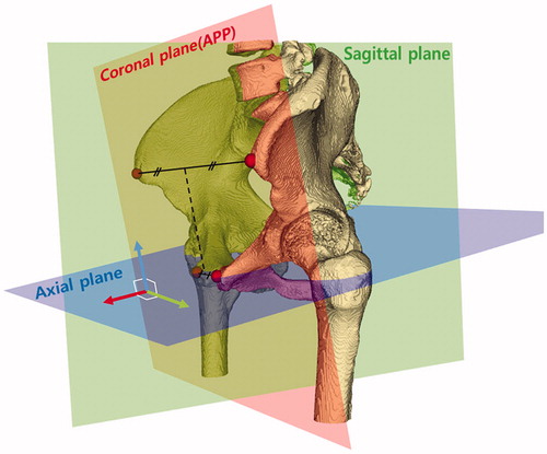
In the first phase, we used an iterative method to determine the pelvic coordinate system according to the method of Lee et al. [8] (Figure 1). This method is useful for measuring the anterior pelvic plane (APP), as it has favorable intra-observer reliability (ICCs =1), and the results from this method are similar to those determined by an experienced surgeon (ICCs ≥0.937). The APP was defined as the tangential plane of the pelvis determined by four pelvic landmarks: the right and left anterior superior iliac spines and the right and left pubic tubercles. Four ROI boxes for each landmark were defined manually by the user in 3-D space. After that, the landmarks were determined by an iterative compensation algorithm of the pelvic pose. The algorithm proceeded by decreasing the difference in angle between the estimated APP of the current iteration and that of the previous iteration. The iteration was stopped when the angle was less than one degree (<1°). Each landmark from the last iteration was the most ventral point with respect to the patient and was defined as the true landmark, and the APP was estimated using the least square method [9]. The sagittal plane was generated by the line connecting the two midpoints of the bilateral anatomical landmarks and the normal vector of the APP. The axial plane was perpendicular to both coronal and sagittal planes.

Figure 1. Three-dimensional pelvic coordinate system. The most ventral points were automatically located on the anterior superior iliac spine and pubic tubercles bilaterally (red points) and were used to establish the three-dimensional pelvic reference frame. The anterior pelvic plane, or coronal plane (red plane), consisted of the anterior superior iliac spine and the pubic tubercle points bilaterally. The sagittal plane (green plane) contained the line (dashed line) connecting the two midpoints of the bilateral anatomical landmarks and was normal to the APP. The axial plane (blue plane) was normal to both coronal and sagittal planes.

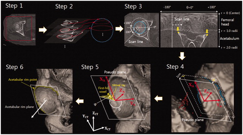
In the second phase, the acetabular rim points, excluding the acetabular notch region, were automatically extracted to represent the acetabular rim plane (Figure 2). This algorithm consisted of six steps. Step 1: Specify the boxes for the regions of interest (ROIs): two ROI boxes for each femoral head were defined by the user. Two regions for one femoral head were specified in the axial slice and the coronal slice, and the overlapped area in 3D was determined as one ROI box. The ROIs were specified separately for each femoral head. Step 2: Evaluate a best-fit sphere for the femoral head: a difference of Gaussian (DoG), which is an image-processing technique to reduce problems from image contrast diversity, was performed for preprocessing [10]. The DoG was an edge-enhance algorithm that involved subtraction of one blurred image of an original image from another, less blurred image of the original. The DoG technique may not always work well for CT images of a femoral head with severe abnormality. After that, the centers and radii of circles, which described the femoral head in each axial slice, were calculated by a Standard Hough Transform (SHT) [11]. A second SHT was then performed to compute the best-fit sphere. Using the estimated sphere, the center coordinates and radius of the best-fit sphere were fitted by the circles in every slice. Step 3: Reconstruct the image slices using the radial scan and extract candidates for the rim points: the pixels on a single radial scan line, which were located in the range of two times the radii from the center of the circle in each slice, were aligned to the corresponding column in a new image (Figure 2), as if unrolling the slice. For example, pixels on the -180° scan line were allocated to the first column in the new image. All pixel intensities were adjusted by 3D tri-linear interpolation. Then, the candidates for the acetabular rim points were extracted in each reconstructed image slice by the corner detection algorithm [12]. Step 4: Generate the pseudo rim plane and the acetabular coordinate system: the pseudo rim plane was generated with the candidates for the acetabular rim points and helped in computing the true acetabular rim plane. The pseudo rim plane was obtained using least squares after removing outliers from the candidates for the acetabular rim points with random sample consensus (RANSAC) [13]. After the pseudo rim plane was generated, the acetabular coordinate system was defined. The center of the coordinate system was the average point of the identified point set. In the acetabular coordinate system, the z-axis ($Z_A$) was a normal vector of the pseudo rim plane, and the x-axis ($X_A$) was the line connecting the center point and an intersection point, which was between the z-axis of the CT volume ($Z_{CT}$) and the pseudo rim plane. Naturally, the y-axis ($Y_A$) was the cross product of $X_A$ and $Z_A$. The pseudo plane and acetabular coordinate system were then moved 1 cm in the direction of the $-Z_A$ axis for the next step. Step 5: Determine the true acetabular rim points: The first-hit voxels along the virtual ray were defined as the true acetabular rim points. As illustrated in Figure 2, the direction of the virtual ray was adjusted by changing the azimuth (θ) and angle (φ) (0 < φ < 90, 0 < θ < 360). The azimuth (θ) was the angle around the X–Y plane of the acetabular coordinate system (pseudo plane), and the angle (φ) was the elevation from the pseudo plane. To avoid the acetabular notch region, these points were excluded. The acetabular notch region was discriminated by the azimuth (θ), which was determined empirically by an orthopedic surgeon. The approximate azimuth corresponding to the acetabular notch region was excluded, with an angular range of 0°–60°. In most cases, this range should discriminate the acetabular notch region well, but in some cases, the notch region may be selected. To address this problem, we included an option to delete the points manually corresponding to the acetabular notch in the 3D view. Step 6: Define the true acetabular rim plane: the plane fitting the acetabular rim points was defined as the true acetabular rim plane by the least squares method.

Figure 2. An algorithm for determining the acetabular rim plane, which consisted of six steps. Step 1: Specifying the ROI for each femoral head (Red box). Step 2: Identifying a best-fit sphere (blue) using planar circles (red) detected by SHT. Step 3: Reconstructing each slice using the scan line. The yellow points detected by the corner detection algorithm were candidates for the acetabular rim points. Step 4: Generating the pseudo plane and acetabular coordinate system. The blue points were selected by a RANSAC algorithm; the red points were determined as outliers. The pseudo plane (dashed line) was determined by blue points, and the plane (solid line) was obtained by moving the pseudo plane 1 cm in the direction of -ZA. Step 5: Determining the true acetabular rim points. The true rim point was defined by a virtual ray. The direction of the virtual ray was adjusted by changing the azimuth (θ) and angle (φ). The first-hit voxels were defined as the true rim points. Step 6: The plane fitting the acetabular rim points (yellow) determined the true acetabular rim plane (white).

The inclination was defined as the angle between the acetabular rim plane and the axial plane of the pelvic coordinate, and anteversion was defined as the angle between the coronal plane and the line that was the normal vector of the acetabular rim plane projected on to the axial plane.

Statistical analysis

Time cost efficiency analysis

To evaluate time cost efficiency, we measured the duration of the two phases – the determination of the pelvic coordinate system and acetabular rim plane. We measured the computation time for each phase, including manual operation. The elapsed time was computed on a Windows 7 laptop PC equipped with a core i7 3.5GHz quad core processor with 16 GB of RAM.

Reliability analysis

Statistical analysis was performed using the CT scans of 20 patients without pathology or a history of surgery in the hip joint. To assess the agreement of our method between trials held at different times, we used our method to calculate the angles from these 20 patients on two occasions at least 4 weeks apart. Each trial was performed independently by the same surgeon. Two data sets (inclination and anteversion) were compared between the trials by calculating the intraclass correlation coefficient (ICC). An ICC value close to 1 indicates excellent agreement when comparing two results. In contrast, an ICC value close to 0 indicates poor agreement [14].

To evaluate inter-observer repeatability, two raters measured acetabular orientation using our algorithm. Each trial was performed independently, and two sets of data (inclination and anteversion) were compared by the ICC.

To evaluate the robustness of our method in relation to patient posture, two result sets were extracted. One was from the original CT volume, and the other was from a CT volume rotated on an arbitrary axis by an angle between 15° and 30°. The ICC values for the two angle sets from each volume were calculated to determine the extent of agreement. We used SPSS software (version 21.0, IBM Inc., Chicago, IL, USA) to calculate the ICCs, using the equation found in [15].

Population data

To understand the morphological difference of the acetabulum by age and sex, we retrospectively reviewed 200 pelvic CT series (400 hips) of Asian patients evaluated for non-orthopedic pathology. The group consisted of 140 women and 60 men, aged between 17 and 91 years. Multiple linear regression analysis was performed to separately investigate the associations of age and sex with acetabular inclination and anteversion. The difference between the angles of the bilateral acetabulum was also examined.

Results

Time-cost efficiency analysis

The elapsed time was 89.04 ± 23.79 s (range, 61.11–141.25 s) for phase 1 and 128.88 ± 9.19 s (115.91–148.92 s) for phase 2. The elapsed time for the overall algorithm was 217.80 ± 28.08 s (180.92–279.94 s) (Table 1). The standard deviation was larger in phase 1 than phase 2. The reason for the large standard deviation in phase 1 is that patient posture was heavily distorted on some CT images, and addressing this issue was time consuming in the iterative process.

Table 1. Elapsed time of the algorithm for two phase including manual operation (n = 20).

Measure	Phase 1^†	Phase 2^‡	Overall process
Mean (sec)	89.04	128.88	217.80
SD* (sec)	23.79	9.19	28.08
Range (sec)	61–141	116–149	181–280

* Standard deviation.

† Pelvic coordinate system determination.

‡ Acetabular rim plane determination.

Reliability analysis

The ICC values for two trials conducted at least 4 weeks apart are presented in Table 2. The results of our method showed excellent consistency with the times of the trial (0.975–0.988) and different raters (0.945–0.976). The agreement in parameter estimates between the original volume and the arbitrarily rotated volume was almost perfect (0.956–0.975). These high ICC values can be attributed to the removal of the major sources of human error arising from manual point selection.

Table 2. ICC values for calculation of the angles on two separate occasions (n = 20).

Measure	Left inclination	Left anteversion	Right inclination	Right anteversion
Trial 1 vs. Trial 2*	0.975	0.988	0.985	0.976
Rater 1 vs. Rater 2^†	0.945	0.976	0.954	0.964
Original volume vs. Rotated volume^‡	0.960	0.967	0.975	0.956

* Intra-observer reliability. The values for each method were calculated for two trials at least 4 weeks apart.

^† Inter-observer reliability. The values for each method were calculated for two raters.

^‡ The rotation angle range on the arbitrary axis was 15°–30°.

Values are ICC scores with 95% confidence intervals (Cronbach alpha values of 0.90–1.00 are considered almost perfect).

Population data

Table 3 summarizes the inclination and anteversion angles of the 200 patients according to age and sex. The mean inclination was 50.03° ± 4.22°, and the mean anteversion was 15.84° ± 4.02°. Ninety percent of patients had acetabular inclination between 40° and 56°; the 90% central range for acetabular anteversion was estimated to be 9°–22°.

Table 3. Acetabular inclination and anteversion by age and gender (n = 200).

Group		# of patients	Inclination angle			Anteversion angle
			Mean	SD*	Range	Mean	SD*	Range
Age <70 years	Males	34	50.64	4.43	37–62	16.07	3.79	4–23
	Females	60	50.11	4.09	39–60	15.48	3.89	9–23
Age ≥70 years	Males	26	51.04	3.96	40–59	16.16	4.28	6–24
	Females	80	50.02	4.43	40–62	16.05	4.23	4–23
All patients		200	50.03	4.22	37–62	15.84	4.02	4–24

* SD = standard deviation.

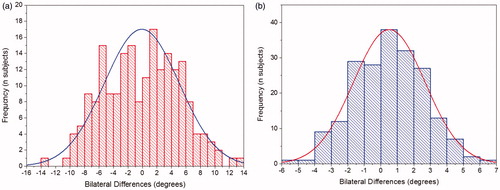
Multiple linear regression analysis with age and sex as covariates indicated that acetabular inclination was not significantly associated with age (p = 0.687) or sex (p = 0.09). There was also no evidence that acetabular anteversion was associated with age (p = 0.383) or sex (p = 0.53). Figures 3 and 4 show the relationships of the inclination and anteversion angles with age and sex, with separate estimated regression lines for males and females superimposed over each plot. Bilateral differences in anatomic anteversion were evenly distributed around a mean of −0.05° (maximum, 14°) (Figure 5(a)). Bilateral differences in anatomic inclination were also evenly distributed around a mean of 0.5° (maximum, 7°) (Figure 5(b)). However, wide variation in acetabular orientation was observed among subjects. For example, acetabular inclination ranged from 36.6° to 61.9° in males and from 39.4° to 61.7° in females. Anteversion ranged from 4.3° to 23.2° in males and from 6.1° to 24.4° in females.

Figure 3. Acetabular inclination by age and sex. Regression analysis indicated no evidence of an association.

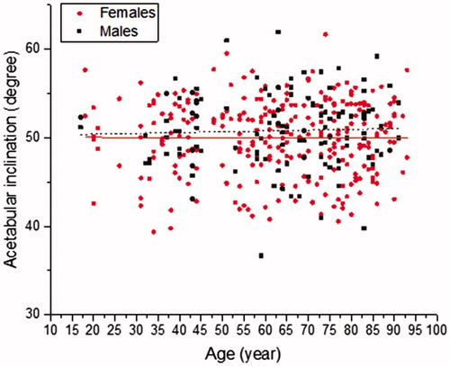
Figure 4. Acetabular anteversion by age and sex. Regression analysis indicated no evidence of an association.

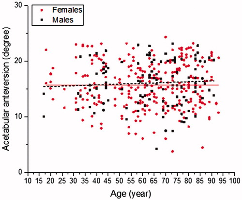
Figure 5. Frequency and magnitude of intra-patient bilateral differences (left minus right). Relative symmetry was shown for (a) anatomic anteversion and (b) anatomic inclination.

Discussion

We developed software to easily and robustly assess the 3D orientation of the acetabulum. The software was integrated with segmentation, anatomical landmark identification, coordinate system establishment, and automatic acetabular orientation measurement, which made the processes faster than conventional methods. It only took about 4 min, including manual specification, to obtain output for a single subject (Table 1). Thus, the software can be efficiently used in a larger population. In addition, we did not use commercial software, so our method was cost efficient.

Intra-observer reliability as measured by the ICC values from two trials conducted at least 4 weeks apart indicated that the results of our method did not differ much between trials (ICC >0.975). The agreement between the results of two raters was slightly lower than the ICC values for intra-observer reliability but was still favorable (ICC >0.945). During extraction of the acetabular rim points in Step 3, selection of the corner points can vary according to ROI specification, and this may affect later steps, such that the ICC values are not 1. Our method was also robust to changes in pelvic position (ICC >0.964). A change in voxel intensities derived from interpolation in the rotation process could affect the pelvic bone model, providing another explanation for why we did not obtain perfect agreement (Table 2).

Using this methodology, we measured acetabular orientation to understand acetabular morphology from 200 CT pelvic scans (400 hips) without apparent hip pathology. Our results indicated that acetabular orientation (inclination, anteversion) might not be associated with age or sex (p > 0.05). These results differ from those of a previous study [16]. Stem et al. reviewed 200 CT images and found that acetabular inclination was associated with age (p = 0.01) but not with sex (p = 0.2), and that acetabular anteversion was associated with both sex (p = 0.01) and age (p = 0.02). However, they selected rim points in a 2D slice, so the results were susceptible to osteophytes and may have been influenced by the direction of the CT slice. Compared with the results reported by Higgins et al. [6], acetabular anteversion and inclination were smaller in our subjects (Table 3). Higgins et al. reported that the average inclination was 56.3°, and the average anteversion was 23.2°. Bilateral differences in acetabular anteversion and inclination were evenly distributed around a mean of −0.05° and 0.5°, respectively.

Understanding the orientation of the acetabulum is important in many orthopedic procedures, including periacetabular osteotomies and the planning, execution, and evaluation of total hip arthroplasties. Inclination and anteversion angles have long been recognized as the two main parameters that define the geometry of the acetabulum. However, inclination and anteversion angles cannot be reliably evaluated on plain radiographs because pelvic tilt can change the measured angles of the native acetabulum and the prosthetic acetabular cup by as much as 10° [17,18]. To overcome these problems, many studies have used 3D anatomical structures for CT volume [19–21]. In general, the angles in 3D are defined by the normal vector of the acetabular rim plane relative to the pelvic coordinate system.

Few studies have investigated methods for determining the pelvic reference plane. Kobashi et al. [22] proposed a method to determine the APP based on anatomical points. With their method, an algorithm using ROIs specified by a quadrant in the CT volume calculates each anatomical point. Although their method applies a calibration algorithm for CT poses using silhouette images, finding two landmarks in narrow structures, such as the pubic tubercle, is difficult. In some cases, one of two pubic tubercle points might not be extracted appropriately. A second method that involves manually selecting anatomical landmarks for the APP can lead to inconsistencies because the ASIS and pubic tubercles are ambiguous anatomical structures that are difficult to represent with specific points. Furthermore, manual selection of landmark points on CT images is tedious, time consuming, and error-prone [23]. A third method uses the sacral base (SB) plane. A crucial step when using this method is segmentation of the SB; however, finding certain boundaries of the SB on CT slices is difficult [21]. A specific segmentation method has not been proposed for this method [20]; therefore, we could not evaluate its efficacy. In the current study, we used an iterative method to robustly determine the pelvic coordinate system [8]. This method is useful for measuring the APP as it is robust, and the results were similar to those determined by an experienced surgeon.

Other computational techniques have been developed to determine the acetabular rim. Jozwiak et al. [20] proposed a manual method to determine the rim points, but manual selection can be inaccurate if not performed by a well-trained user. The method in Lubovsky et al. [23] did not include a process to remove the region of the acetabular notch, which might lead to inaccurate results. Higgins et al. [6] selected the most lateral distal points in the captured region as the rim points. Their method is simple to apply, but additional software is needed to complete manual segmentation, which is a time-consuming process. To reduce these problems, we developed an algorithm to automatically extract the acetabular rim plane. For reference, some studies have described the normal acetabulum as a nearly perfect hemisphere, with the centers of the acetabulum and femoral head in almost the same location [24]. Therefore, our approach modeling the femoral head as a sphere is reasonable.

Murray et al. [1] described a nomogram showing the relationship between anatomical, radiographic, and operative measurements of cup inclination and anteversion. We used the anatomical definition, which they report can accurately describe the orientation of the normal and dysplastic acetabulum. The measurement using this definition is consistent with the application of our study in that it could be used for dysplastic diagnostic procedures.

Our study had several limitations. First, a method that involves user-selected ROIs can be tedious. Overcoming this limitation will require an automated method for specifying each region. This remains challenging, however, because the landmarks do not provide clues that allow the region in the CT volume to be identified by image processing. Second, we analyzed a relatively small population, which included fewer male subjects (n = 60) than females (n = 140). Third, this study was conducted in a population of Asians. Further study is needed to assess whether our method is affected by ethnic differences. Fourth, our software has not been commercialized, so the reported technique cannot yet be used in the wider community.

As part of our future work, we plan to apply our method to subjects with implants. An accuracy test of our method using cadavers or phantoms would also be useful. Zhang et al.[4] compared the differences between standardized models based on predetermined parameters and computationally measured 3D acetabular orientation. However, the standardized model is a virtual model that assumes the acetabular rim is a hemi-sphere, quite different from the true shape of the acetabular rim. Thus, we cannot ensure accuracy using their model.

In conclusion, our method showed excellent reliability for determining acetabular orientation, as it is robust, fast, and easily applicable to larger populations. In addition, the results of the analysis of acetabular orientation by age and sex can be used as a reference in various diagnostic procedures in orthopedics.

Additional information

Funding

This research was supported by the Basic Science Research Program through the National Research Foundation of Korea (NRF) funded by the Ministry of Education [2018R1D1A1B07048957].

References

- Murray DW. The definition and measurement of acetabular orientation. J Bone Joint Surg Br. 1993;75(2):228–232.
- Pinoit Y, May O, Girard J, et al. [Low accuracy of the anterior pelvic plane to guide the position of the cup with imageless computer assistance: variation of position in 106 patients]. Rev Chir Orthop Reparatrice Appar Mot. 2007;93(5):455–460.
- Lembeck B, Mueller O, Reize P, et al. Pelvic tilt makes acetabular cup navigation inaccurate. Acta Orthop. 2005;76(4):517–523.
- Zhang H, Wang Y, Ai S, et al. Three-dimensional acetabular orientation measurement in a reliable coordinate system among one hundred Chinese. PLoS One. 2017;12(2):e0172297.
- Lubovsky O, Wright D, Hardisty M, et al. Acetabular orientation: anatomical and functional measurement. Int J Comput Assist Radiol Surg. 2012;7(2):233–240. doi: 10.1007/s11548-011-0648-3.
- Higgins SW, Spratley EM, Boe RA, et al. A novel approach for determining three-dimensional acetabular orientation: results from two hundred subjects. J Bone Joint Surg Am. 2014;96(21):1776–1784. doi: 10.2106/JBJS.L.01141.
- Schroeder W, Martin K, Lorensen B. An object-oriented approach to 3D graphics. Vol. 429. Upper Saddle River: Prentice hall; 1997.
- Lee C, Kim Y, Kim HW, et al. A robust method to extract the anterior pelvic plane from CT volume independent of pelvic pose. Comput Assist Surg. 2017;22(1):20–26. doi: 10.1080/24699322.2017.1293737.
- Abdi H. The method of least squares. Encyclopedia of Measurement and Statistics. Thousand Oaks (CA): Sage; 2007.
- Basu M. Gaussian-based edge-detection methods-a survey. IEEE Trans Syst Man Cybern C. 2002;32(3):252–260.
- Cao M, Ye C, Doessel O, et al. Spherical parameter detection based on hierarchical Hough transform. Pattern Recognit Lett. 2006;27(9):980–986.
- Harris C, Stephens M, editors. A combined corner and edge detector. Alvey vision conference; 1988; Citeseer.
- Fischler MA, Bolles RC. Random sample consensus: a paradigm for model fitting with applications to image analysis and automated cartography. Commun ACM. 1981;24(6):381–395.
- Fleiss JL, Cohen J. The equivalence of weighted kappa and the intraclass correlation coefficient as measures of reliability. Educ Psychol Meas. 1973;33(3):613–619.
- Shrout PE, Fleiss JL. Intraclass correlations: uses in assessing rater reliability. Psychol Bull. 1979;86(2):420.
- Stem ES, O’Connor MI, Kransdorf MJ, et al. Computed tomography analysis of acetabular anteversion and abduction. Skeletal Radiol. 2006;35(6):385–389.
- Anda S, Svenningsen S, Grøntvedt T, et al. Pelvic inclination and spatial orientation of the acetabulum: a radiographic, computed tomographic and clinical investigation. Acta Radiol. 1990;31(4):389–394.
- Muller O, Reize P, Trappmann D, et al. Measuring anatomical acetabular cup orientation with a new X-ray technique. Comput Aided Surg. 2006;11(2):69–75. doi: 10.3109/10929080600640618.
- Babisch JW, Layher F, Amiot L-P. The rationale for tilt-adjusted acetabular cup navigation. The J Bone Joint Surg. 2008;90(2):357–365.
- Jozwiak M, Rychlik M, Musielak B, et al. An accurate method of radiological assessment of acetabular volume and orientation in computed tomography spatial reconstruction. BMC Musculoskelet Disord. 2015;16:42. doi: 10.1186/s12891-015-0503-8. PubMed PMID: 25887277; PubMed Central PMCID: PMC4351831.
- Haas B, Coradi T, Scholz M, et al. Automatic segmentation of thoracic and pelvic CT images for radiotherapy planning using implicit anatomic knowledge and organ-specific segmentation strategies. Phys Med Biol. 2008;53(6):1751.
- Kobashi S, Fujimoto S, Nishiyama T, et al. Robust pelvic coordinate system determination for pose changes in multidetector-row computed tomography images. Int J Fuzzy Logic Intell Syst. 2010;10(1):65–72.
- Lubovsky O, Peleg E, Joskowicz L, et al. Acetabular orientation variability and symmetry based on CT scans of adults. Int J Comput Assist Radiol Surg. 2010;5(5):449–454. doi: 10.1007/s11548-010-0521-9.
- Song W, Ou Z, Zhao D, et al., editors. Computer-aided modeling and morphological analysis of hip joint. Bioinformatics and Biomedical Engineering, 2007. ICBBE 2007. The 1st International Conference on; 2007: Piscataway, NJ: IEEE.