Super resolution reconstruction for medical image based on adaptive multi-dictionary learning and structural self-similarity

Abstract

To improve the quality of the super-resolution (SR) reconstructed medical images, an improved adaptive multi-dictionary learning method is proposed, which uses the combined information of medical image itself and the natural images database. In training dictionary section, it uses the upper layer images of pyramid which are generated by the self-similarity of low resolution images. In reconstruction section, the top layer image of pyramid is taken as the initial reconstruction image, and medical image’s SR reconstruction is achieved by regularization term which is the non-local structure self-similarity of the image. This method can make full use of the same scale and different scale similar information of medical images. Simulation experiments are carried out on natural images and medical images, and the experimental results show the proposed method is effective for improving the effect of medical image SR reconstruction.

Keywords:

• Super-resolution reconstruction
• medical image
• improved adaptive multi-dictionary learning
• non-local structural similarity

1. Introduction

With the continuous innovation of medical imaging technology and computer technology, medical image processing is becoming important in clinical diagnosis. It can help doctors fully understand the structure of the internal pathology of patients, and then an accurate treatment plan is developed. High-quality medical images can not only improve the level of clinical diagnosis, but also provide necessary support for medical research, teaching, surgery, etc. Commonly used methods of super-resolution (SR) reconstruction are interpolation methods, such as B-spline and bicubic interpolation etc. Through SR reconstruction, the clarity of medical images and the correctness of disease diagnosis, can be improved. Thereby it can help doctors to perform precise treatment on patients.

A single HR image is generated by one or more low-resolution images in the same scene based on SR method [1]. And for SR method, it is the biggest difficulty to recover high frequency information lost during process of getting LR inputs [2,3].

Yang et al. [4] propose a SR algorithm based on sparse representation. In this algorithm, FSS (Feature-Sign Search) method plans to generate low-resolution (LR) and high-resolution (HR) dictionaries by using the patch pairs of HR and LR image. LR dictionary produces the spare coefficients of LR image patches, and it uses the coefficients to produce the HR image patches based on the HR dictionary.

For each local patch, pre-learned dictionaries from a dataset of high quality example patches are selected based on Dong [5]. In the process of reconstruction, non-local structure self-similarity (NLSS) and autoregressive model are considered as the regularization term. Dong’s method uses the self-similarity of the image that increases the accuracy and reliability accessed to the information. Therefore, it still uses the image database to train the global dictionary, and it cannot be sparse representation for all image patches. In order to further improve the reconstruction effect, A SR method based on adaptive multi-dictionary learning (MDL) was proposed by Pan [6]. Firstly, patches of LR image pyramid which are packed into some categories are classified into one of these groups, if they meet special conditions. And then, corresponding dictionaries are generated for each group based on MDL.

This paper proposes an improved method based on adaptive MDL and structural self-similarity. In this method, we use the pyramid generated by structural self-similarity upper layer images as samples instead of Pan’s method. It uses the pyramid decomposition to obtain samples when training a dictionary, which will achieve more self-similar information of the different scales. In addition, the paper uses the top layer image of pyramid as the initial reconstruction image. SR image is reconstructed by regularization term using the non-local structure self-similarity of image. It also employs self-similar information of the same scale to reconstruct image. Experimental results demonstrate that the HR medical image reconstructed by the proposed method has good effect for medical images.

2. SR model

2.1. SR model based on sparse representation

Supposing $\Phi \in {\mathfrak{R}}^{N\times M}$ $(N<M)$is an over-complete dictionary of M prototype signal-atoms, a sparse linear combination of these atoms can represent a signal. The signal vector can be expressed as: (1) $$x\approx \Phi \alpha$$(1) $\alpha \in {\mathfrak{R}}^M$ is the sparse coefficient with very few $\left(\ll M\right)$ nonzero term. Solving an $l_0$-minimization problem can calculate the sparse decomposition coefficient, and it can be formulated as: (2) $$\alpha =\underset{\alpha }{\arg \min }{\parallel \alpha \parallel }_0,s.t.{\parallel x-\Phi \alpha \parallel }_2\le \epsilon$$(2) where $\left|\right|•|{|}_0$ is a pseudo norm that counts the number of non-zero entries in $\alpha$, and approximation error is influenced by a small constant $\epsilon$. Minimization $l_0$ is converted to the convex $l_1$ -minimization. It is an issue about NP-hard combinatorial optimization. According to sparse coding problem, $l_1$ -norm is summarized as follows: (3) $$\alpha =\underset{\alpha }{\arg \min }{\parallel \alpha \parallel }_1,s.t.{\parallel x-\Phi \alpha \parallel }_2\le \epsilon$$(3)

Eq. (3)(3) $$\alpha =\underset{\alpha }{\arg \min }{\parallel \alpha \parallel }_1,s.t.{\parallel x-\Phi \alpha \parallel }_2\le \epsilon$$(3) also can be written as the form of Lagrange polynomials: (4) $$\alpha =\underset{\alpha }{\arg \min }\{{\parallel x-\Phi \alpha \parallel }_2^2+\lambda {\parallel \alpha \parallel }_1\}$$(4) where $\lambda$ represents the regularization parameter, it is a constant.

The single image SR problem can be presented as: a HR image $X$ of the same scene can be recovered by giving a LR image $Y$. Assuming the LR image is the version of the solution $X$. And the version is blurred and down-sampled: (5) $$Y=DBX$$(5) where $B$ is a fuzzy filter, and $D$ is a lower sampling operator. The process of solving $X$ by $Y$ is the process of image SR reconstruction, which is to solve the following least squares problem: (6) $$X=\underset{X}{\arg \min }{\parallel Y-DBX\parallel }_2^2$$(6)

The sparse representation prior on small patches $x$ of $X$ is used to make HR images $X$ satisfy the reconstruction constraint for a given LR input $Y$.

$x$ is an image column vector reshaped from image $X$. $R_i$ is a extracting-matrix, whose function is extracting patch $x_i$ from $X$. $x_i=R_{i}X$, $i=1,2,\dots ,N$ is the $i^{th}$ patch (size: $\sqrt{n}\times \sqrt{n}$) vector of $x$.$\left\{{\Phi }_k\right\}$, $k=1,2,\dots ,M$ is defined to be a set of orthonormal sub-dictionaries. ${\widehat{x}}_i={\Phi }_{k_i}{\alpha }_i$ can approximately express the sparse coding $x_i$, $\left|\right|{\alpha }_i|{|}_1\le T$ and the reconstructed patches ${\widehat{x}}_i$ are averaged to reconstruct the whole image $x$. And it can be described as: (7) $$\widehat{X}=\Phi \circ \alpha ={\left(\sum _{i=1}^N{R}_i^{\text{T}}{R}_i\right)}^{-1}\sum _{i=1}^N\left(R_i^{\text{T}}{\Phi }_{k_i}{\alpha }_i\right)$$(7) where $\alpha$ represents a collection of all ${\alpha }_i$. And $\Phi$ represents a collection of all sub-dictionaries $\left\{{\Phi }_k\right\}$.

For $Y=DBX$, recovering the original image $X$ from $Y$ is our goal. A super-resolution reconstruction model based on sparse representation through Eqs. (6)(6) $$X=\underset{X}{\arg \min }{\parallel Y-DBX\parallel }_2^2$$(6) and (7)(7) $$\widehat{X}=\Phi \circ \alpha ={\left(\sum _{i=1}^N{R}_i^{\text{T}}{R}_i\right)}^{-1}\sum _{i=1}^N\left(R_i^{\text{T}}{\Phi }_{k_i}{\alpha }_i\right)$$(7) can be summarized as follows: (8) $$\widehat{\alpha }=\underset{\alpha }{\arg \min }\{{\parallel Y-DB\Phi \circ \alpha \parallel }_2^2+\lambda {\parallel \alpha \parallel }_1\}$$(8) $l_1$-norm sparsity regularization term $\left|\right|\alpha |{|}_1$ is weighted by the constant $\lambda$. And the $l_0$-norm sparsity is closer to the reweighted $l_1$-norm sparsity than using a constant weight according to Ref [13]. Therefore, Eq. (8)(8) $$\widehat{\alpha }=\underset{\alpha }{\arg \min }\{{\parallel Y-DB\Phi \circ \alpha \parallel }_2^2+\lambda {\parallel \alpha \parallel }_1\}$$(8) can be summed up as: (9) $$\widehat{\alpha }=\underset{\alpha }{\arg \min }\{{\parallel Y-DB\Phi \circ \alpha \parallel }_2^2+\sum _{i=1}^N\sum _{j=1}^n{\lambda }_{i,j}\parallel {\alpha }_{i,j}\parallel \}$$(9) where ${\lambda }_{i,j}$ represents the weight assigned to ${\alpha }_{i,j}$, ${\alpha }_{i,j}$ represents the coefficient associated with the $j^{th}$ atom of ${\Phi }_{k_i}$. ${\lambda }_{i,j}$ that can be obtained by the following formula: (10) $${\lambda }_{i,j}=\frac{c}{\left|{\alpha }_{i,j}^{\left(l\right)}\right|+\epsilon }$$(10) where $c$ is a constant, ${\alpha }_{i,j}^{(l)}$ is an estimated value of the first $l$ iteration of ${\alpha }_{i,j}$, and $\epsilon$ is a small constant.

2.2. SR model combined with structure self-similarity

In general, many duplicate images contain a lot of redundant information. And the quality of reconstructed images is significantly improved. Therefore, a non-local self-similar regularization term based on sparsity of the image SR framework is proposed. In the whole image $\widehat{X}$, similar patches $x_i^l\left(l=1,2,\dots ,L\right)$ are found for each local patch $x_i$. If $e_i^l={\parallel {\widehat{x}}_i-{\widehat{x}}_i^l\parallel }_2^2\le t$, similar patch will choose a patch $x_i^l$. ${\widehat{x}}_i$, ${\widehat{x}}_i^l$ are the current estimated value based on the preset threshold $t$. And the patch ${\widehat{x}}_i^l$ within the first L closest patches is also selected to ${\widehat{x}}_i$, where L is also a preset threshold. The center pixel of patch $x_i$ and $x_i^l$ are ${\chi }_i$ and ${\chi }_i^l$, respectively. The weighted average of ${\chi }_i^l$, i.e., ${\sum }_{l=1}^L{b}_i^l{\chi }_i^l$ is predicted based on ${\chi }_i$. The weight $b_i^l$, which is allocated to ${\chi }_i^l$ is assumed as $b_i^l=\hspace{0.17em}\text{exp}\hspace{0.17em}(-e_i^l/h)/{\sum }_{l=1}^L\hspace{0.17em}\text{exp}\hspace{0.17em}(-e_i^l/h)$, where $h$ is a weight control factor. In this paper, the difference between ${\chi }_i$ and ${\widehat{\chi }}_i$ is used as a regularization term, i.e. ${\parallel {\chi }_i-{\sum }_{l=1}^L{b}_i^l{\chi }_i^l\parallel }_2^2$. So the sparse representation and structure self-similarity are combined to obtain the image super resolution reconstruction model: (11) $$\begin{array}{c}\widehat{\alpha }=\underset{\alpha }{\arg \min }\{{\parallel Y-DB\Phi \circ \alpha \parallel }_2^2\\ +\sum _{i=1}^N\sum _{j=1}^n{\lambda }_{i,j}\left|{\alpha }_{i,j}\right|+\eta \cdot \sum _{i=1}^N\parallel {\chi }_i-\sum _{l=1}^L{b}_i^l{\chi }_i^l\parallel \}\end{array}$$(11) where $\eta$ is to balance the contribution of non-local regularization, it is a constant.

Then by merging the first term and third term, the simplified form of Eq. (11)(11) $$\begin{array}{c}\widehat{\alpha }=\underset{\alpha }{\arg \min }\{{\parallel Y-DB\Phi \circ \alpha \parallel }_2^2\\ +\sum _{i=1}^N\sum _{j=1}^n{\lambda }_{i,j}\left|{\alpha }_{i,j}\right|+\eta \cdot \sum _{i=1}^N\parallel {\chi }_i-\sum _{l=1}^L{b}_i^l{\chi }_i^l\parallel \}\end{array}$$(11) can be expressed as (12) $$\widehat{\alpha }=\underset{\alpha }{\arg }\min \left\{{\parallel \tilde{Y}-F\Phi \circ \alpha \parallel }_2^2+\sum _{i=1}^N\sum _{j=1}^n{\lambda }_{i,j}\parallel {\alpha }_{i,j}\parallel \right\}$$(12) where (13) $$\tilde{Y}=\left[\begin{array}{c}Y\\ 0\end{array}\right],\hspace{1em}F=\left[\begin{array}{c}DB\\ \eta \cdot \left(I-A\right)\end{array}\right],$$(13) A expresses the weight matrix, and $I$ expresses the identity matrix.

3. Acquisition and training of adaptive multi-dictionary samples

3.1. Selection of samples

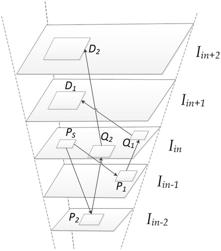
In order to get the missing high-frequency information, it is necessary to obtain the dictionary that contains the high-frequency information. In this paper, the dictionary training samples is consisted of image itself to be processed and the natural image database. The natural image database is mainly to select high resolution images with rich texture details. For the image itself, we generate the image pyramid by self-similarity to produce the training samples. It contains the image's own information, and the upper layer images of pyramid are selected as the samples of a dictionary. The principle of generating the image pyramid by self-similarity is as follows.

Figure 1 shows the input image $I_{in}$, and we generate LR images $I_{in-k}$ ($k=1,2,\dots ,m$) as the lower layer images of the pyramid firstly. In the lower-resolution images ($I_{in-1}$ or $I_{in-2}$), some similar patches ($P_1$ and $P_2$) are searched where $P_s$ is a source patch in $I_{in}$. A corresponding region ($Q_1$ or $Q_2$) in $I_{in}$ are determined for each patch ($P_1$ or $P_2$). The corresponding region ($D_1$ or $D_2$) depends on two factors: (1) the area of source patch $P_s$, and (2) the layer index of the found patch (−1 of $I_{in-1}$ or −2 of $I_{in-2}$). In the end, $Q_1$ is moved to the corresponding position of the enlarged area $D_1$, and $Q_2$ is also the case. $P_s$ is not exactly like $P_k$, and $Q_k$ is not exactly like $D_k$. So $D_k$ can be obtained by $Q_k$ weighted, and the formula is as follows: (14) $$D_k={\sum \omega }_k{Q}_k$$(14) where their weights are (15) $${\omega }_k=\hspace{0.17em}\text{exp}\hspace{0.17em}\left(-{\parallel P_s-P_k\parallel }^2/{\sigma }^2\right)$$(15)

Figure 1. The image pyramid generated by self-similarity.

And $\sigma$ controls the degree of similarity. $I_{in+1}$ and $I_{in+2}$ are denoted in the HR images in Figure 1. $I_{in+1}$ and $I_{in+2}$, which have some copied patches, have many undetected areas (i.e., in the image pyramid, some similar patches are not found by source patches in $I_{in}$). Uncovered area will be filled with the back projection to improve image resolution based on method [6].

3.2. Training of adaptive multi-dictionary

As mentioned above, the dictionary has an important impact on the reconstruction results. In order to enrich the high frequency information contained in the dictionary, this paper adopts the method of combining the image itself and the natural images database. Firstly, we take the upper layer images of pyramid as the training samples $S$. The semantic information is conveyed by the edge of image which is sensitive to human visual system. The high-pass filtering is used to obtain the feature of each patch with size $\sqrt{n}\times \sqrt{n}$ for the training samples $S$ of clustering. Blocks only with a certain edge structure are used in dictionary learning to exclude the smooth patches from training. We select the intensity variance of image patch which is better than a threshold $\Delta$. The selected image patch, denoted by $s_i,i=1,2,\dots ,m$, and $g_i,i=1,2,\dots ,m$ is the high frequency component of ${\tilde{s}}_i$. The high frequency component patches $g_i$ are clustered into K clusters by K-means algorithm, which is denoted by $C_k=\left\{g_1^k,g_2^k,\dots ,g_{m_k}^k\right\}$, $k=1,2,\dots ,K$, where $m_k$ is the number of samples for each class that guarantee ${\sum }_{k=1}^K{m}_k=m$. Then we compute class centers ${\mu }_k=\frac{1}{m_k}{\sum }_{i=1}^{m_k}{g}_i^k$ and radius $r_k=\max {\parallel g_i^k-{\mu }_k\parallel }_2,i=1,\dots ,m_k$ for each class.

Similar with the upper layer images of pyramid, the high-pass filtering is used for the images of the natural image database. Abundant image patches are cropped from the natural images. The size of the image patch is $\sqrt{n}\times \sqrt{n}$, and we selected the patches whose intensity variances are better than a threshold $\Delta$. The selected image patch is denoted by ${\tilde{s}}_i,i=1,2,\dots ,n$, and ${\tilde{g}}_i,i=1,2,\dots ,n$ is the high frequency component of ${\tilde{s}}_i$. Then we compute the distance between ${\tilde{g}}_i$ and the class centers ${\mu }_k$, which is denoted by $d_i^k$. If $\min \left(d_i^k\right)<\delta r_k$, ${\tilde{g}}_i$ is added to $C_k$, otherwise the image block is abandoned, where $\delta$ is a parameter that is used to control the similarity degree between the image blocks and the class centers. After the above operation, the samples are expanded, and each type of expanded sample is recorded as $C_k=\{g_1^k,g_2^k,\dots ,g_{q_k}^k\}$, where $q_k$ is the number of samples after the expansion.

Then, according to the high frequency component samples $C_k$, we can find the corresponding image block sample matrix$S_k=[s_1^k,s_2^k,\dots ,s_{q_k}^k]$ $k=1,2,\dots ,K$. The following objective function can formulate the design of sub-dictionary ${\Phi }_k$. (16) $$({\widehat{\Phi }}_k,{\widehat{\Lambda }}_k)=\underset{{\Phi }_k,{\Lambda }_k}{\arg \min }\left\{{\parallel S_k-{\Phi }_k{\Lambda }_k\parallel }_F^2+\lambda {\parallel {\Lambda }_k\parallel }_1\right\}$$(16) where ${\Lambda }_k$ is the representation coefficient matrix, and $\lambda$ is the parameter controlling the degree of sparsity. In order to reduce the amount of computation, the principal component analysis (PCA) is used to calculate the main parts for each sub-dataset $S_k$. An orthogonal transformation matrix $P_k$, which is generated by applying PCA, is set the dictionary, and it meets $Z_k=P_k^{\text{T}}{S}_k$. Then we will have ${\parallel S_k-P_k{Z}_k\parallel }_F^2$=${\parallel S_k-P_k{P}_k^{\text{T}}{S}_k\parallel }_F^2$ = 0. In order to obtain a dictionary ${\Phi }_r=[p_1,p_2,\dots ,p_r]$, the first $r$ which is the most important eigenvectors in $P_k$ is separated. In this way, the relationship of $l_1$-norm regularization term and $l_2$-norm approximation term in Eq. (16)(16) $$({\widehat{\Phi }}_k,{\widehat{\Lambda }}_k)=\underset{{\Phi }_k,{\Lambda }_k}{\arg \min }\left\{{\parallel S_k-{\Phi }_k{\Lambda }_k\parallel }_F^2+\lambda {\parallel {\Lambda }_k\parallel }_1\right\}$$(16) is more balanced. The reconstruction error ${\parallel S_k-{\Phi }_r{\Lambda }_r\parallel }_F^2$ will increase the decrease of $r$ according to Eq. (16)(16) $$({\widehat{\Phi }}_k,{\widehat{\Lambda }}_k)=\underset{{\Phi }_k,{\Lambda }_k}{\arg \min }\left\{{\parallel S_k-{\Phi }_k{\Lambda }_k\parallel }_F^2+\lambda {\parallel {\Lambda }_k\parallel }_1\right\}$$(16) . Considering the term ${\parallel {\Lambda }_r\parallel }_1$ will reduce, the best value $r_0$ of $r$ can be prescribed for: (17) $$r_0=\underset{r}{\arg \min }\left\{{\parallel S_k-{\Phi }_r{\Lambda }_r\parallel }_F^2+\lambda {\parallel {\Lambda }_r\parallel }_1\right\}$$(17) where $\lambda$ is the weight of the $l_1$ norm sparse regularization term ${\parallel \alpha \parallel }_1$. In the end, the sub-dictionary which is learned from sub-dataset $S_k$ is ${\Phi }_k=[p_1,p_2,\dots ,p_{r_0}]$, $k=1,2,\dots ,K$.

Finally, we seek an adaptive dictionary for the image patches to be reconstructed. Considering spanning the adaptive sparse domain, a sub-dictionary is assigned adaptively to each partial patch of $x$. $X$ needs to be estimated in advance, because it is not known at the beginning. We can take the top layer image of pyramid as the initial estimation of $X$. $\widehat{X}$ represents the estimate of $X$, and ${\widehat{x}}_i$ represents the local patch of $\widehat{X}$. For the centroid ${\mu }_k$, considering the high-pass filtered patch of ${\widehat{g}}_i$, the best fitted sub-dictionary to ${\widehat{x}}_i$ is generated, which is of each cluster available. For ${\widehat{x}}_i$, the dictionary is influenced by the minimum distance between ${\widehat{g}}_i$ and ${\mu }_k$, i.e. (18) $$k_i=\underset{k}{\arg \min }{\parallel {\widehat{g}}_i-{\mu }_k\parallel }_2$$(18)

3.3. Algorithm Flow

In the paper, in order to solve Eq. (12)(12) $$\widehat{\alpha }=\underset{\alpha }{\arg }\min \left\{{\parallel \tilde{Y}-F\Phi \circ \alpha \parallel }_2^2+\sum _{i=1}^N\sum _{j=1}^n{\lambda }_{i,j}\parallel {\alpha }_{i,j}\parallel \right\}$$(12) , we use the iterative shrinkage algorithm [7]. The algorithm flow chart is shown in Figure 2.

Figure 2. The algorithm flow chart of this paper.

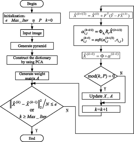
The overall algorithm process is as follows:

1. Initialization:

   1. By the descending process of the image, we determine the down-sampling matrix $D$ and the blurring matrix $B$;

   2. The sub-dictionary ${\Phi }_{k_i}$ is established by PCA, in which samples from the natural images and the upper layer images of the pyramid by structural self-similarity property are established;

   3. The weight matrix $A$ of the non-local structure self-similarity is obtained by searching the similar image patches of the same scale in the image;

   4. The termination error $e$, the maximal iteration number $Max\_\mathit{\text{Iter}}$, the constant of controlling non-local regularization term $\eta$, and the condition of updating parameters $P$ are presented;

2. It is iterated on $k$ until $k\ge Max\_\mathit{\text{Iter}}$ or ${\parallel {\widehat{X}}^{(k)}-{\widehat{X}}^{(k-1)}\parallel }_2^2/N\le e$ is satisfied.

   1. The current estimation is updated using Eq. (19)(19) $${\widehat{X}}^{(k+1/2)}={\widehat{X}}^{\left(k\right)}+F^{\text{T}}(\tilde{Y}-F{\widehat{X}}^{\left(k\right)})$$(19) : (19) $${\widehat{X}}^{(k+1/2)}={\widehat{X}}^{\left(k\right)}+F^{\text{T}}(\tilde{Y}-F{\widehat{X}}^{\left(k\right)})$$(19)

   2. The sparse representation coefficients are updated using Eq. (20)(20) $${\alpha }_{i,j}^{(k+1/2)}={\Phi }_{k_i}{R}_i{\widehat{X}}^{(k+1/2)}$$(20) and Eq. (21)(21) $${\alpha }_{i,j}^{(k+1)}=\mathit{\text{soft}}({\alpha }_{i,j}^{(k+1/2)},{\tau }_{i,j})$$(21) : (20) $${\alpha }_{i,j}^{(k+1/2)}={\Phi }_{k_i}{R}_i{\widehat{X}}^{(k+1/2)}$$(20) (21) $${\alpha }_{i,j}^{(k+1)}=\mathit{\text{soft}}({\alpha }_{i,j}^{(k+1/2)},{\tau }_{i,j})$$(21) where $\mathit{\text{soft}}(\cdot ,{\tau }_{i,j})$ is a soft function of thresholding, and its threshold is ${\tau }_{i,j}$; (22) $$\mathit{\text{soft}}(x,\tau )=\mathrm{sgn}\left(x\right)\max \left(\left|x\right|-\tau ,0\right)$$(22) where $\mathrm{sgn}(x)$ is a sign function;

   3. Re-update the current estimation ${\widehat{X}}^{(k+1)}=\Phi \circ {\alpha }^{(k+1)}$;

   4. If $\mathrm{mod}(k,P)=0$, the improved estimate ${\widehat{X}}^{(k+1)}$ is used to update the matrix $A$ and the adaptive sparse domain of $X$.

4. Experimental results and analysis

This section mainly presents the results of the SR reconstruction of medical images by this method. It also performs three sets of experiments in both noiseless and noisy cases. The three sets of experimental images (Head1, Head2, and Chest) are actually taken by the hospital, including MRI images and CT images. In the experiments, the degraded LR image is generated by a 7 × 7 gaussian kernel and an original image with a standard deviation of 1.6 make the degraded LR image. Then the image is down sampled by a factor of 3. Firstly, the low resolution color images are converted to ycbcr format. Finally, the bicubic interpolator is applied to the color components. We compare our method with two most advanced methods: the bicubic interpolation method and the ASDS method [8]. The statistical experimental results are analyzed and discussed to verify the advantages of this method for medical image’s SR reconstruction. The results with noiseless are shown in Figures 3–5 and Table 1. The results with noise are shown in Figures 6–8 and Table 2.

Figure 3. Comparison of the reconstructed images of various methods for noiseless medical image (1(1) $$x\approx \Phi \alpha$$(1) ) (a) Original image (b) LR image (c) Bicubic (d) ASDS (e) Our.

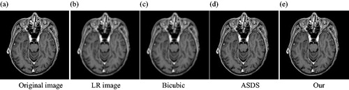
Figure 4. Comparison of the reconstructed images of various methods for noiseless medical image (2(2) $$\alpha =\underset{\alpha }{\arg \min }{\parallel \alpha \parallel }_0,s.t.{\parallel x-\Phi \alpha \parallel }_2\le \epsilon$$(2) ) (a) Original image (b) LR image (c) Bicubic (d) ASDS (e) Our.

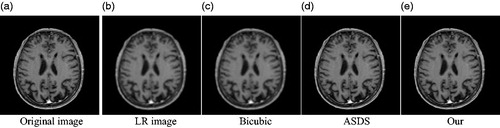
Figure 5. Comparison of the reconstructed images of various methods for noiseless medical image (3(3) $$\alpha =\underset{\alpha }{\arg \min }{\parallel \alpha \parallel }_1,s.t.{\parallel x-\Phi \alpha \parallel }_2\le \epsilon$$(3) ) (a) Original image (b) LR image (c) Bicubic (d) ASDS (e) Our.

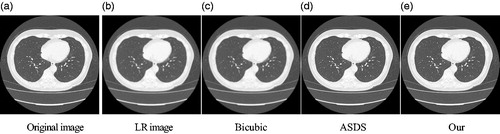
Figure 6. Comparison of the reconstructed images of various methods for noisy medical image (1(1) $$x\approx \Phi \alpha$$(1) ) (a) Original image (b) LR image (c) Bicubic (d) ASDS (e) Our.

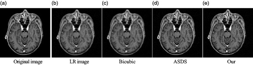
Figure 7. Comparison of the reconstructed images of various methods for noisy medical image (2(2) $$\alpha =\underset{\alpha }{\arg \min }{\parallel \alpha \parallel }_0,s.t.{\parallel x-\Phi \alpha \parallel }_2\le \epsilon$$(2) ) (a) Original image (b) LR image (c) Bicubic (d) ASDS (e) Our.

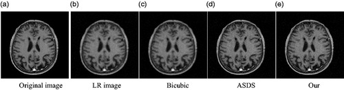
Figure 8. Comparison of the reconstructed images of various methods for noisy medical image (3(3) $$\alpha =\underset{\alpha }{\arg \min }{\parallel \alpha \parallel }_1,s.t.{\parallel x-\Phi \alpha \parallel }_2\le \epsilon$$(3) ).

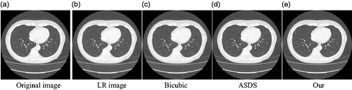
Table 1. Comparison of PSNR (dB)/SSIM of the medical images ($\sigma =0$) based on various methods.

Test Images	Bicubic	ASDS	Our
Head1	22.26	27.14	27.40
	0.7371	0.8906	0.8970
Head2	24.15	29.46	29.86
	0.8005	0.9136	0.9166
Chest	21.23	24.16	24.66
	0.4490	0.5597	0.5666

Table 2. Comparison of PSNR (dB)/SSIM of the medical images ($\sigma =5$) based on various methods.

Test Images	Bicubic	ASDS	Our
Head1	22.09	25.03	25.51
	0.5662	0.6310	0.6385
Head2	23.87	27.13	27.51
	0.6046	0.6288	0.6306
Chest	21.09	23.40	23.83
	0.3742	0.4254	0.4391

Firstly, Figures 3–8 show the reconstructed results for the three images of Head1, Head2, and Chest. The texture of the head and the texture of lungs in the chest can be observed clearly. The blur and noise conditions are greatly improved. Compared with the bicubic algorithm and the ASDS method, the medical images reconstructed by our method are of better quality, and more detailed.

Secondly, we compare our method with the two method for medical images respectively for quantitatively prove the advantages of our method. Evaluating the experimental results based on various methods use the SSIM and PSNR [9]. The greater value of the PSNR indicates the quality of the reconstructed image and the reconstructed results are better. SSIM evaluates the structure differences between the reconstructed image and the high resolution image by SR. The greater the value of SSIM is, the better the reconstructed result will be. Table 1 and Table 2 list the SSIM and PSNR results, and it can be seen from the results in the table that the method presented in this paper has good results.

In addition, we compare the complexity and time consumption of the bicubic interpolation method, the ASDS method and our method. The calculation formula of time complexity is $T\left(n\right)=O(f(n))$, where $f(n)$ is the frequency of the sentence with the largest frequency in the algorithm. The program of time consuming test method is run on Matlab R2014b, and the average time consumption of the 512 × 512 pixel test chart is calculated. The test results are shown in Table 3.

Table 3. Comparison of complexity.

Item	Bicubic	ASDS	Our
Complexity	$O\left(n^3\right)$	$O\left(n^3\right)$	$O\left(n\right)$
Time consumption	2.74s	3.84s	2.52s

Furthermore, we give the experimental results on the public image library for fully prove the advantages of our method. We randomly selected 20 high quality natural images from the sample database. Figure 9 shows the results of comparing our method with two most advanced methods: the bicubic interpolation method and the Yang method. From the result we can see the proposed method results achieve the most visual effect, which is more clearly compared with the other algorithms because more details are restored. Secondly, for quantitatively demonstrate the advantages of our method, we use PSNR and SSIM to evaluate the experimental results based on various methods. Table 4 list the SSIM and PSNR consequence of these algorithms, where it can be seen that our method is more effective than others. The average PSNR gains over other methods are up to 3.4 dB and 2.57 dB. Compared with other methods, the average value of the SSIM gains up to 0.0706 and 0.0455, respectively.

Figure 9. Comparison of the reconstructed images of various methods for Butterfly image (a) Original image (b) Bicubic (c) Yang (d) Our.

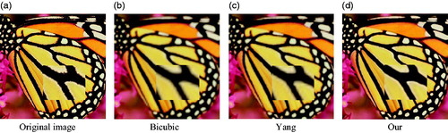
Table 4. Comparison of PSNR (dB)/SSIM of the reconstructed images based on various method.

Test Images	Bicubic	Yang	Our
hat	28.27/0.8005	29.09/0.8263	31.44/0.8793
castle	25.61/0.7712	26.12/0.7935	26.98/0.8292
Input3	27.36/0.8892	28.51/0.9163	33.03/0.9643
average	27.08/0.8203	27.91/0.8454	30.48/0.8909

5. Conclusions

In this paper, we introduce a single image super resolution reconstruction method based on adaptive MDL and structural self-similarity. The proposed method is the improvement for the existing adaptive MDL method. In this method, the image pyramid is generated by structural self-similarity, and the pyramid upper layer images are as samples, which will contain more self-similar information of the different scales than directly conducting the pyramid decomposition for the image itself. In addition, the paper uses the top layer image of pyramid as the initial reconstruction image and the image SR reconstruction uses the non-local structure self-similarity of the image as the regularization term. It also added the self-similar information of the same scale to the reconstruction image. Experimental results demonstrate that our method achieves better results in terms of all the visual perception and the parameters of PSNR and SSIM compared with multiple super resolution reconstruction methods.

Disclosure statement

No potential conflict of interest was reported by the authors.

Additional information

Funding

This study was sponsored by the National Natural Science Foundation of China (NSFC) (grant no. 61601325), the Tianjin Natural Science Foundation (grant no. 17JCQNJC01400), and Supported by the Program for Innovative Research Team in University of Tianjin (grant no. TD13-5034).

References

- Xie B, Duan ZM, Ma PG, et al. SR reconstruction algorithm of infrared image based on dynamic pyramid model[J]. Infrared and Laser Eng. 2018;001(1):277–282.
- Pan ZX, Yu J, Hu SX, et al. Super-resolution based on compressive sensing and structural self-similarity for remote sensing images. IEEE Transac Geosci Remote Sens. 2013;51(9):4864–4876.
- Zhao H, Wei JX, Pang ZH, et al. Wave-front coded super-resolution imaging technique. Infrared and Laser Eng. 2016;45(4):227–236.
- Yang J, Wright J, Huang TS, et al. Image super-resolution via sparse representation. IEEE Transac Image Proc. 2010;19(11):2861.
- Dong WS, Zhang L, Shi GM, et al. Image deblurring and super-resolution by adaptive sparse domain selection and adaptive regularization. IEEE Transac Image Proc. 2011;20(7):1838–1857.
- Pan ZX, Yu J, Xiao CB, et al. Single image super resolution based on adaptive multi-dictionary learning. Acta Electronica Sinica. 2015;43(2):209–216.
- Dong WS, Zhang L, Lukac R, et al. Sparse representation based image interpolation with nonlocal autoregressive modeling. IEEE Transac Image Proc. 2013;22(4):1382–1394.
- Zhang A, Guan C, Jiang H, et al. An image super-resolution scheme based on compressive sensing with PCA sparse representation. In: Shi YQ, Kim HJ, editors. The international workshop on digital forensics and watermarking 2012. Berlin Heidelberg: Springer; 2013.
- Zhang X, Zhou W, Duan Z. Image super-resolution reconstruction based on fusion of K-SVD and semi-coupled dictionary learning. IEEE Signal and Information Processing Association Summit and Conference; 2017 December 13–16, Jeju, South Korea.