Novel joint algorithm based on EEG in complex scenarios

Abstract

At present, in the field of electroencephalogram (EEG) signal recognition, the classification and recognition in complex scenarios with more categories of EEG signals have gained more attention. Based on the joint fast Fourier transform (FFT) and support vector machine (SVM) methods, this study proposed a novel EEG signal-processing joint method for the complex scenarios with 10 classifications of EEG signals. Moreover, a comprehensive efficiency formula was put forward. The formula considered the accuracy and time consumption of the joint method. This new joint method could improve the accuracy and comprehensive efficiency of multiclass EEG signal recognition. The new joint approach used standardization for data preprocessing. Feature extraction was performed by combining FFT and principal component analysis methods. EEG signals were classified using the weighted k-nearest nenighbour method. In this study, experiments were conducted using public datasets of brainwave 0-9 digits classification. The result demonstrated that the accuracy and comprehensive efficiency of the novel joint method were 84% and 87%, respectively, which were better than those of the existing methods. The precision rate, recall rate, and F1 score of the novel joint method were 89%, 85%, and 0.85, respectively. In conclusion, the proposed joint method was effective in a complex scenario for multiclass EEG signal recognition.

Keywords:

• Accuracy
• complex scenario
• comprehensive efficiency
• EEG
• joint method

Introduction

Electroencephalography (EEG) signal is an electrical signal generated by spontaneous electrical activity of hundreds of millions of neurons in the brain. It contains abundant information about brain activity. EEG is an intuitive reflection of the state and function of the brain and has the characteristics of being complex, time-varying, and volatile [1–4]. At the same time, the brain is also an important organ of the human body, which has important research value. To facilitate the application of EEG signals in clinical studies and practical use, various studies have proposed the noninvasive brain-computer interface (BCI) technology [5–8].

The EEG-based noninvasive BCI technology is a novel human-computer interaction method. It is independent of human peripheral nerves and muscle tissues, and can realize the communications and controls between the human brain and computer or other peripheral devices. After the researchers extracted the signal characteristics of the acquired EEG signals, they usually used the machine learning methods for classification and recognition [9–13]. The ultimate goal is to send instructions and control external devices. At present, the time-domain and frequency-domain analysis methods [14–16], such as fast Fourier transform (FFT), are commonly used methods of EEG signal processing. Then, machine learning methods, such as support vector machine (SVM) and artificial neural network, are used to classify EEG signals [17–20].

Several studies have reported on the classification of EEG data. For example, Giannakaki et al. [9] collected EEG signals by inducing different emotions and obtained three different types of EEG signals representing calm, positive, and negative emotions. They used wavelet transform combined with SVM method to classify the signals. The accuracy of the recognition result reached 75.12%. Yildiz et al. [17] studied the classification of EEG signals of epileptic patients and normal people. They extracted features from the time domain and frequency domain, such as power spectrum, and then used machine learning methods, SVM, and multilayer perceptron to classify the EEG signals. The accuracy was more than 90%. Other studies have also achieved good results in terms of classification of EEG signals.

At present, studies on the classification of EEG signals mostly focus on the simple recognition scenario of EEG signals of less than five categories, but relatively less research has been done on the classification of more categories of EEG signals. Although a dataset of 10-class EEG signals exists, very few studies have reported on such data to date. This dataset can be used to study EEG recognition of a complex scenario. More importantly, the classification accuracy and time complexity of existing EEG signal classification methods can still be improved. In the field of EEG recognition, two widely used joint classification methods exist: FFT-based joint method [21] and SVM-based joint method [22]. Therefore, based on the existing methods, this study proposed a novel joint method for classifying EEG signals in a complex scenario.

1. Methods

In this section, two existing joint methods have been introduced: one is based on FFT, and the other on SVM. Also, the proposed novel joint method has been described in detail.

1.1. FFT joint method

FFT is a mathematical method used in frequency-domain analysis of signals. It is also widely used in the feature extraction of EEG signals. Akin [23] proposed a joint method based on FFT, which was applied to analyze EEG signals of watching 3D television by five normal volunteers. First, the method normalized the EEG signals and then used FFT and wavelet packet transform methods to process the signals. This method was a classical joint method for EEG signal processing.

As the most common data preprocessing method, normalization can effectively reduce the difficulty in processing data and lower the time complexity of subsequent methods. The calculation formula is as follows: (1) $$x^{*}=\frac{x-x_{\min }}{x_{\max }-x_{\min }}$$(1) where $x$ is the data point of samples, $x_{\max }$ is the maximum value in the data, and $x_{\min }$ is the minimum value in the data. $x^{\ast }$ is the result after the normalization, and it ranges from 0 to 1.

After data preprocessing, discrete Fourier transform was used for feature extraction. The formula is as follows: (2) $$X\left(k\right)=\sum _{n=0}^{N-1}x\left(n\right)W_N^{\mathit{nk}}(k=0,1,\dots ,N-1)$$(2)

and (3) $$W_N=e^{-j\frac{2\pi }{N}}$$(3) where $N$ is the number of signal data points, $x(n)$ represents the sequence of discrete digital signals, $W_N$ is the twiddle factor, and $X(k)$ is the result of the transformation.

Then, the obtained spectral distribution was taken as the feature vector. Finally, the k-NN method [24] for classification was used.

This classical joint method was widely used in EEG signal analysis. However, when the data volume was large and the dimension was high, the joint method had a large time complexity. Therefore, the comprehensive performance of the method needs to be improved.

1.2. SVM joint method

The SVM method is a commonly used classification method in the field of machine learning. It can transform the linear inseparable samples of low-dimensional input space into linear separable samples of high-dimensional feature space. This method was also widely used in classifying EEG signals. Subasi and Gursoy [25] proposed an SVM-based joint method. The method was applied to classify and recognize EEG signals in the brain of patients with epileptic seizures and normal individuals. First, they normalized the EEG signals and then employed the primary component analysis (PCA) method to extract features using the SVM method for classification. This method provided a classical joint classification method for EEG recognition.

The SVM joint method first normalizes the EEG data and then uses the PCA [26] method to extract features. Let the set of training samples be $\{x_1,x_2,\dots ,x_n\};$ then the average vector of the sample set is (4) $$\overline{x}=\frac{1}{n}\sum _{i=1}^n{x}_i$$(4)

The covariance formula is (5) $$\text{Cov}(x_i,x_j)=\frac{1}{n}{(x_i\hspace{0.17em}-\hspace{0.17em}\overline{x})}^{\mathrm{T}}(x_j\hspace{0.17em}-\hspace{0.17em}\overline{x})$$(5)

Thus, a covariance matrix is obtained, and it is used for PCA [27].

The PCA method can effectively reduce the dimension and lower the time complexity at the same time. After PCA processing, the reduced data are regarded as the feature vector, and the SVM method [28–31] is used for feature classification.

The SVM method can solve the small sample, nonlinear, and high-dimensional data classification problem well. Combined with the PCA method for dimension reduction and feature extraction, the method has a large advantage in time complexity. However, the adaptability of SVM to multiclass data and large dataset is poor, and the accuracy is not ideal, leaving a large space for improvement.

1.3. Novel joint method

Based on the aforementioned two joint methods, this study proposed a new joint method. It combined the FFT and PCA methods for feature extraction and used the weighted k-NN method for final classification. The weighted method [32,33] could overcome the influence of data noise and data imbalance and make higher classification accuracy. The PCA method could eliminate the noise in the data and reduce the feature dimension. The process of this method is as follows (Figure 1):

Figure 1. Novel joint method flow chart.

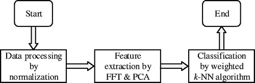
Step 1: Normalization method was used to preprocess the original EEG signals

Step 2: FFT operation was performed on the data. The sequence was divided into two groups according to parity, and the number of values in each group was $N/2-1.$ Then, there is (6) $$X\left(k\right)=\sum _{r=0}^{N/2-1}{x}_1\left(r\right)W_N^{2rk}+W_N^k\sum _{r=0}^{N/2-1}{x}_2(r\left)W_N^{2rk}\right(k=0,1,\dots ,N-1)$$(6) and (7) $$x\left(2r\right)=x_1\left(r\right),x(2r+1)=x_2\left(r\right),r=0,1,\dots ,N/2-1$$(7)

Using the reducibility of coefficient $W_N,$ the following expression was obtained: (8) $$X\left(k\right)=X1\left(k\right)+W_N^k{X}_2\left(k\right)$$(8) where $X_1(k)$ and $X_2(k)$ have N/2 points with a period of N/2. In this way, the frequency-domain information of the EEG signals could be obtained. Then, PCA was performed on the frequency-domain features. Putting Equation (8)(8) $$X\left(k\right)=X1\left(k\right)+W_N^k{X}_2\left(k\right)$$(8) into Equation (5)(5) $$\text{Cov}(x_i,x_j)=\frac{1}{n}{(x_i\hspace{0.17em}-\hspace{0.17em}\overline{x})}^{\mathrm{T}}(x_j\hspace{0.17em}-\hspace{0.17em}\overline{x})$$(5) , where the training sample set is $\{X(0),X(1),\dots ,X(N-1)\},$ the following expression was obtained: (9) $$\text{Cov}\left(X\left(i\right),X\left(j\right)\right)=\frac{1}{N}{\left(X\left(i\right)-\overline{X}\right)}^T\left(X\left(j\right)-\overline{X}\right)$$(9)

and (10) $$X=\frac{1}{N}\sum _{i=0}^{N-1}X\left(i\right)$$(10)

This formula is the mean vector of the training dataset $\{X(0),X(1),\dots ,X(N-1)\},$ and $\text{Cov}(X(i),X(j))$ is the i-th row and j-th column element of the covariance matrix.

Then, the eigenvalues and corresponding eigenvectors of the covariance matrix were calculated. After that, the eigenvectors were arranged into a matrix from top to bottom according to the corresponding eigenvalues from small to large. Finally, the first few rows of the matrix were taken to form the transformation matrix. Through this transformation matrix, feature vectors could be projected to low-dimensional feature spaces.

Step 3: The data obtained from the FFT and dimension reduction were taken as final feature vectors, and the weighted k-NN method was used for feature classification. The method assumed that all feature samples were in the n-dimensional space, and each sample was represented as the vector $<a_1(x),a_2(x),\dots ,a_n(x)>,$ where $a_r(x)$ denotes the value of the r-th attribute of sample $x.$ Then, the similarity between the two samples was measured by the Euclidean distance. Let $w_k$ be the characteristic weight value and m be the number of attribute values of each sample. The weighting method can be referred from a previous study [34], and the formula can be simplified as follows: (11) $$d(x_i,x_j)=\sum _{k=1}^m{w}_k{\left[a_k\left(x_i\right)-a_k\left(x_j\right)\right]}^2$$(11)

2. Materials and comprehensive efficiency formula

2.1. Data acquisition

The International 10–20 System was used as the reference standard for electrode placement. The data in the experiment were collected from the public dataset: MindBigData (http://www.mindbigdata.com/opendb/). A multichannel EEG acquisition equipment Emotiv Insight was used for the purpose. The positions of the signals collected in the 10–20 System were AF3, AF4, T7, T8, and Pz. The equipment recorded the EEG signals of participants when they observed the numbers 0–9 in a period of 2 s. A total of 65,250 pieces of data were collected as the dataset. The EEG signal distribution corresponding to stimulus digits 0–9 is shown in Table 1.

Table 1. Distribution table of the EEG samples according to digit stimulation.

Digit stimulation	Number of EEG samples
0	6,305
1	6,740
2	6,535
3	6,605
4	6,620
5	6,460
6	6,425
7	6,470
8	6,590
9	6,500
Total	65,250

In this experiment, the five-fold cross-validation method [35,36] was used to make full use of all samples and evaluate the joint method model. In this method, the data were divided into five disjoint subsets, one of which was selected as the test set and the other four as training sets for each time. The number of test data was 13,050, and the number of training data was 52,200. Therefore, every experiment was carried out five times to ensure the reliability and stability of the results. Moreover, the time consumption and relevant performance evaluation metrics of each experiment were analyzed.

2.1. Comprehensive efficiency

Two important parameters were used to judge the performance of the joint method: one was the time consumption for the method operation, and the other was the final classification accuracy of the method. To assess the joint method better, a comprehensive efficiency formula was designed based on the information of time consumption and accuracy. Suppose N methods are present, and the accuracy of the i-th method is $m_i,$ in the interval [0, 1]. The normalized time information parameter is $t_i.$ The formula is (12) $$t_i=\frac{t_{i0}-t_{{}_{\min }}}{t_{\max }-t_{\min }}$$(12) where the time consumption before normalization processing is represented by $t_{i0},$ and $t_{\min }$ and $t_{\max }$ represent the minimum and maximum values of time consumption, respectively, before normalization.

Because $t_i$ was normalized, its value was in the range [0, 1]. The comprehensive performance of the method was inversely proportional to the time complexity and proportional to the accuracy approximately. To facilitate the calculation, $1-t_i$ was used in the formula. For avoiding the zero value, $(1-t_i)+0.1$ was adopted. The final comprehensive efficiency formula was as follows: (13) $$P_i=\left[(1-t_i)+0.1\right]\times m_i$$(13)

The variable $P_i$ is the synthesis efficiency of the ith method, which was used to evaluate the synthesis performance of the joint method.

3. Experiments and results

This study used cross-validation to perform five independent experiments using three EEG classification joint methods. Then, time consumption and other performance evaluation metrics were compared, and the average was calculated as the final reference measurement.

For these three joint methods, the parameter tuning was conducted on relative models and classifiers. After tuning, the better parameters for these classifiers were chosen. For the k-NN classifier in the FFT joint method, the number of neighbors was set as 5. For the PCA method in the SVM joint method, the number of components to keep was 20; for the SVM method, the “rbf” kernel function was applied, and the penalty parameter C was 0.4. For the PCA method in the novel joint method, the number of components to keep was 20; and for the k-NN classifier, the number of neighbors was set as 2.

3.1. Average time complexity analysis

Table 2 compares the time consumption of the three joint methods. The computer processor used was Intel Core i7-4790, and the main frequency was 3.60 GHz. Table 2 shows that, in the process of classifying EEG signals, the time consumed by the FFT joint method was obviously longer than that for the SVM joint method and the new joint method proposed in this study. Also, the time for the new joint method was a little longer than that for the SVM joint method because the SVM method does not undergo complex FFT operation. In addition, the new joint method consumed less time because PCA analysis was used to reduce the data dimension. Under the premise of high classification accuracy, the time consumption of the new joint method was acceptable.

Table 2. Time consumption of the three joint methods (second).

Method	Exp. 1	Exp. 2	Exp. 3	Exp. 4	Exp. 5	AVG
FFT joint method	164.94	161.80	162.84	166.63	163.21	163.88
SVM joint method	30.85	32.82	29.42	32.50	31.56	31.43
New joint method	39.81	42.53	40.28	41.98	39.99	40.92

Comparing the average time consumption of the three joint methods, it was found that the time consumption for the new joint method and the SVM joint method was close, while that of the FFT joint method was about three times that for the former two methods. Therefore, the new joint method performed well in terms of time consumption.

3.2. Classification performance analysis

Accuracy is a classification effectiveness evaluation indicator often used in classification problems. The comparison of the accuracy of three joint methods in the complex case of classifying 10-category EEG is shown in Table 3. It is obvious that the classification accuracy of the FFT joint method was higher than that of the SVM joint method, and the accuracy of the new joint method was better than that of the FFT joint method and the SVM joint method. The average accuracy of the new joint method improved by 6% compared with that of the FFT joint method, and by 20% compared with that of the SVM joint method. This showed that the combination of FFT and PCA could obtain the main features of EEG signals and better characterize EEG signals. At the same time, the application of the weighted k-NN method also improved the classification accuracy.

Table 3. Accuracy of the three joint methods.

Digit	FFT joint method					SVM joint method					New joint method
	Exp. 1	Exp. 2	Exp. 3	Exp. 4	Exp. 5	Exp. 1	Exp. 2	Exp. 3	Exp. 4	Exp. 5	Exp. 1	Exp. 2	Exp. 3	Exp. 4	Exp. 5
0	0.77	0.79	0.82	0.77	0.80	0.67	0.72	0.71	0.68	0.69	0.85	0.84	0.88	0.80	0.82
1	0.78	0.77	0.82	0.76	0.81	0.70	0.69	0.69	0.68	0.70	0.87	0.86	0.85	0.81	0.83
2	0.83	0.78	0.76	0.81	0.78	0.68	0.66	0.70	0.68	0.71	0.83	0.83	0.87	0.84	0.85
3	0.84	0.77	0.79	0.79	0.78	0.69	0.71	0.72	0.69	0.72	0.84	0.82	0.86	0.83	0.84
4	0.77	0.78	0.79	0.76	0.83	0.67	0.67	0.74	0.67	0.67	0.88	0.85	0.90	0.83	0.84
5	0.80	0.79	0.84	0.77	0.82	0.69	0.75	0.68	0.69	0.72	0.86	0.84	0.84	0.83	0.87
6	0.79	0.80	0.82	0.76	0.80	0.71	0.72	0.72	0.65	0.71	0.84	0.85	0.89	0.83	0.82
7	0.78	0.76	0.83	0.78	0.77	0.66	0.69	0.74	0.67	0.73	0.84	0.84	0.84	0.84	0.83
8	0.83	0.75	0.82	0.79	0.75	0.71	0.67	0.67	0.69	0.67	0.85	0.83	0.83	0.85	0.84
9	0.81	0.80	0.81	0.81	0.76	0.72	0.72	0.73	0.70	0.68	0.84	0.84	0.84	0.84	0.86
AVG	0.80	0.78	0.81	0.78	0.79	0.69	0.70	0.71	0.68	0.70	0.85	0.84	0.86	0.83	0.84

In the five cross-validation experiments, the average accuracy of the FFT joint method, SVM joint method, and new joint method was 0.79, 0.70, and 0.84, respectively.

Table 3 shows that the average accuracy of the three methods from high to low was as follows: the novel joint method, FFT joint method, and SVM joint method. Therefore, the new joint method had better performance in terms of accuracy.

In addition, to ensure the performance and credibility of the methods, other evaluation metrics, such as precision, recall, F1 score, and kappa coefficient, were also compared.

As the accuracy metric simply calculates the proportion of the sample with the correct prediction, it does not distinguish between the prediction results of different categories and does not consider the case of sample imbalance. Therefore, other more effective metrics are needed. Precision and recall are two metrics widely used in the field of information retrieval and statistical classification to evaluate the quality of results. Then these two metrics were adopted for performance evaluation of the three joint methods in EEG signal recognition.

Precision calculated the proportion of all “correctly retrieved” for all “actually retrieved.” The metric was used for performance evaluation when the number of samples in different categories was not completely equal. The comparison of the precision rate of the three methods is shown in Table 4. It was apparent that the precision rate of the SVM joint method was higher than that of the FFT joint method, and the precision of the new joint method was better than that of the SVM joint method. It could be seen that the average precision of the new joint method improved by 25% compared with that of the FFT joint method, and by 17% compared with that of the SVM joint method. This showed that the application of the weighted k-NN method also improved the classification performance.

Table 4. Precision rate of the three joint methods.

Digit	FFT joint method					SVM joint method					New joint method
	Exp. 1	Exp. 2	Exp. 3	Exp. 4	Exp. 5	Exp. 1	Exp. 2	Exp. 3	Exp. 4	Exp. 5	Exp. 1	Exp. 2	Exp. 3	Exp. 4	Exp. 5
0	0.71	0.72	0.71	0.69	0.72	0.77	0.77	0.76	0.75	0.76	0.89	0.88	0.88	0.89	0.88
1	0.71	0.71	0.73	0.71	0.70	0.76	0.76	0.76	0.76	0.76	0.88	0.89	0.90	0.89	0.90
2	0.72	0.70	0.71	0.71	0.72	0.76	0.76	0.76	0.75	0.77	0.89	0.89	0.89	0.89	0.89
3	0.70	0.72	0.72	0.70	0.71	0.76	0.75	0.75	0.76	0.78	0.89	0.89	0.89	0.89	0.89
4	0.72	0.73	0.73	0.72	0.73	0.76	0.75	0.76	0.75	0.74	0.89	0.89	0.89	0.89	0.89
5	0.72	0.71	0.72	0.73	0.73	0.75	0.76	0.77	0.76	0.76	0.89	0.89	0.89	0.89	0.89
6	0.71	0.71	0.71	0.70	0.72	0.76	0.76	0.76	0.76	0.75	0.89	0.89	0.89	0.89	0.89
7	0.71	0.72	0.72	0.72	0.72	0.77	0.76	0.76	0.78	0.77	0.89	0.89	0.89	0.89	0.89
8	0.72	0.71	0.72	0.72	0.72	0.76	0.75	0.76	0.77	0.76	0.89	0.88	0.89	0.90	0.90
9	0.71	0.71	0.71	0.72	0.71	0.76	0.75	0.76	0.77	0.77	0.89	0.88	0.90	0.89	0.89
AVG	0.71	0.71	0.72	0.71	0.72	0.76	0.76	0.76	0.76	0.76	0.89	0.89	0.89	0.89	0.89

In the five cross-validation experiments, the average precision of the FFT joint method, SVM joint method, and new joint method was 0.71, 0.76, and 0.89, respectively.

Recall stands for the ratio of “correctly retrieved” for all “should be retrieved”. It is also an effective performance metric when the sample category is unbalanced. The comparison of the recall rate of the three-method classifications is shown in Table 5. The table shows that the recall rate of the SVM joint method was higher than that of the FFT joint method, and the recall rate of the new joint method was better than that of the SVM joint method. The average recall rate of the new joint method improved by 25% compared with that of the FFT joint method, and by 20% compared with that of the SVM joint method. This indicated that the new joint method was an effective joint method for EEG signal classification.

Table 5. Recall rate of the three joint methods.

Digit	FFT joint method					SVM joint method					New joint method
	Exp. 1	Exp. 2	Exp. 3	Exp. 4	Exp. 5	Exp. 1	Exp. 2	Exp. 3	Exp. 4	Exp. 5	Exp. 1	Exp. 2	Exp. 3	Exp. 4	Exp. 5
0	0.68	0.69	0.68	0.67	0.68	0.72	0.72	0.72	0.71	0.73	0.86	0.85	0.85	0.85	0.85
1	0.66	0.67	0.68	0.67	0.66	0.65	0.67	0.71	0.67	0.69	0.84	0.85	0.86	0.85	0.86
2	0.68	0.67	0.68	0.67	0.68	0.69	0.70	0.70	0.71	0.71	0.85	0.85	0.85	0.85	0.85
3	0.67	0.68	0.68	0.67	0.67	0.72	0.73	0.73	0.70	0.72	0.85	0.82	0.85	0.85	0.84
4	0.68	0.69	0.69	0.68	0.69	0.73	0.69	0.68	0.70	0.71	0.85	0.86	0.84	0.85	0.86
5	0.68	0.68	0.68	0.68	0.69	0.71	0.73	0.73	0.72	0.75	0.85	0.86	0.85	0.85	0.85
6	0.67	0.67	0.66	0.66	0.67	0.71	0.72	0.70	0.72	0.71	0.85	0.85	0.84	0.85	0.85
7	0.67	0.68	0.68	0.68	0.68	0.70	0.71	0.70	0.68	0.68	0.85	0.85	0.84	0.84	0.85
8	0.67	0.67	0.68	0.68	0.67	0.72	0.72	0.72	0.72	0.70	0.85	0.84	0.85	0.85	0.86
9	0.67	0.67	0.67	0.68	0.67	0.74	0.73	0.71	0.73	0.75	0.86	0.86	0.86	0.86	0.86
AVG	0.67	0.68	0.68	0.68	0.68	0.71	0.71	0.71	0.71	0.71	0.85	0.85	0.85	0.85	0.85

In the five cross-validation experiments, the average recall of the FFT joint method, SVM joint method, and new joint method was 0.68, 0.71, and 0.85, respectively.

Precision and recall are mutually influential, although an ideal situation arises when both are high. In general, when precision is high, recall is low, or recall is low, but precision is high. Therefore, in practice, it is often necessary to make trade-offs according to specific situations. For example, in the case of general search, the precision rate is raised under the premise of ensuring recall. Moreover, for disease monitoring, anti-spam, and so on, the recall rate is improved under the premise of ensuring the precision rate. However, sometimes, it is required to balance the two, and then the F1 score indicator can be adopted. It is assumed that the precision and recall rates are as high as possible in classifying EEG signals.

The F1 score is a compromise between precision and recall, and it is the harmonic mean of precision rate and recall rate. The comparison of F1 score of the three methods is shown in Table 6. Table 6 shows that the F1 score of the SVM joint method exceeded that of the FFT joint method, and the F1 score of the new joint method was higher than that of the SVM joint method. The average F1 score of the new joint method increased by 29% compared with that of the FFT joint method, and by 21% compared with that of the SVM joint method. This suggested that the new joint method could obviously improve the classification quality.

Table 6. F1 score of the three joint methods.

Digit	FFT joint method					SVM joint method					New joint method
	Exp. 1	Exp. 2	Exp. 3	Exp. 4	Exp. 5	Exp. 1	Exp. 2	Exp. 3	Exp. 4	Exp. 5	Exp. 1	Exp. 2	Exp. 3	Exp. 4	Exp. 5
0	0.67	0.67	0.66	0.66	0.67	0.71	0.70	0.71	0.70	0.72	0.85	0.85	0.85	0.85	0.84
1	0.65	0.65	0.67	0.65	0.65	0.62	0.64	0.69	0.64	0.68	0.83	0.85	0.85	0.85	0.86
2	0.67	0.66	0.66	0.66	0.66	0.66	0.69	0.69	0.70	0.70	0.85	0.85	0.85	0.85	0.85
3	0.65	0.66	0.67	0.66	0.66	0.71	0.72	0.72	0.68	0.71	0.85	0.85	0.85	0.85	0.84
4	0.67	0.67	0.67	0.67	0.68	0.72	0.68	0.66	0.68	0.71	0.85	0.85	0.85	0.85	0.85
5	0.67	0.67	0.67	0.67	0.68	0.70	0.72	0.72	0.70	0.75	0.85	0.85	0.85	0.85	0.85
6	0.65	0.65	0.65	0.64	0.66	0.69	0.71	0.69	0.71	0.69	0.85	0.85	0.85	0.85	0.85
7	0.66	0.67	0.67	0.67	0.66	0.68	0.69	0.68	0.65	0.66	0.84	0.85	0.84	0.84	0.85
8	0.66	0.65	0.67	0.68	0.66	0.70	0.71	0.72	0.71	0.69	0.85	0.84	0.84	0.86	0.86
9	0.66	0.65	0.66	0.66	0.66	0.74	0.73	0.70	0.73	0.75	0.85	0.84	0.86	0.86	0.86
AVG	0.66	0.66	0.67	0.66	0.65	0.69	0.70	0.70	0.69	0.71	0.85	0.85	0.85	0.85	0.85

In the five cross-validation experiments, the average F1 score of the FFT joint method, SVM joint method, and new joint method was 0.66, 0.70, and 0.85, respectively.

For a multiclass classification problem, measures such as the accuracy or precision/recall do not provide the complete description of the performance of the classifier in this study. Moreover, when faced with a problem with imbalanced classes, accuracy can be misleading, and then precision, recall, and F1 scores are the other options. However, the F1 score measure does not have an excellent intuitive explanation, other than it being the harmonic mean of precision and recall. Thus, the kappa coefficient was used, which is a very good measure that can handle both multiclass and imbalanced class problems well.

The kappa coefficient can better represent the performance of the multiclassification model based on the confusion matrix of classification results. It is generally thought to be a more robust measure than the simple percent agreement calculation. Moreover, the definition of kappa coefficient is as follows: (14) $$\kappa =\frac{p_0-p_e}{1-p_e}$$(14) where $p_0$ is the relative observed agreement among raters (identical to accuracy) and $p_e$ is the hypothetical probability of chance agreement, using the observed data to calculate the probabilities of each observer randomly seeing each category. Moreover, the formula of $p_e$ is as follows: (15) $$p_e=\frac{1}{N^2}\sum _k{n}_{\cdot k}{n}_{k\cdot }$$(15) where $N$ is the number of items; and for category k, $n_{\cdot k}$ denotes the number of samples predicted to be category $k,$ and $n_{k\cdot }$ denotes the number of samples of category $k.$

The comparison of kappa coefficient of the three method classifications is shown in Table 7. The table shows that the kappa coefficient of the new joint method was better than that of the FFT joint method and the SVM joint method. The average kappa coefficient of the new joint method increased by 94% compared with that of the FFT joint method, and by 23% compared with that of the SVM joint method. The experimental results showed that the new joint method could effectively improve the results of classifying EEG signals in the complex scenario.

Table 7. Kappa coefficient of the three joint methods.

Digit	FFT joint method					SVM joint method				New joint method
	Exp. 1	Exp. 2	Exp. 3	Exp. 4	Exp. 5	Exp. 1	Exp. 2	Exp. 3	Exp. 4	Exp. 5	Exp. 1	Exp. 2	Exp. 3	Exp. 4	Exp. 5
0	0.37	0.37	0.35	0.33	0.37	0.45	0.44	0.44	0.43	0.46	0.71	0.71	0.71	0.70	0.69
1	0.33	0.34	0.36	0.34	0.33	0.31	0.34	0.42	0.34	0.40	0.68	0.71	0.73	0.70	0.72
2	0.37	0.34	0.36	0.35	0.36	0.38	0.41	0.41	0.43	0.43	0.70	0.71	0.71	0.71	0.70
3	0.33	0.35	0.36	0.34	0.35	0.44	0.46	0.45	0.40	0.44	0.70	0.70	0.70	0.70	0.69
4	0.37	0.38	0.38	0.36	0.38	0.46	0.39	0.37	0.40	0.43	0.71	0.71	0.68	0.71	0.72
5	0.36	0.36	0.37	0.37	0.38	0.42	0.46	0.46	0.44	0.50	0.70	0.71	0.71	0.70	0.70
6	0.34	0.36	0.33	0.32	0.35	0.42	0.44	0.41	0.45	0.41	0.70	0.71	0.69	0.70	0.71
7	0.35	0.37	0.36	0.37	0.36	0.41	0.41	0.40	0.37	0.38	0.70	0.71	0.70	0.69	0.71
8	0.35	0.34	0.36	0.38	0.35	0.44	0.44	0.45	0.45	0.41	0.71	0.68	0.70	0.72	0.73
9	0.35	0.33	0.35	0.36	0.34	0.48	0.47	0.43	0.47	0.50	0.71	0.70	0.73	0.72	0.72
AVG	0.35	0.36	0.36	0.35	0.36	0.42	0.43	0.42	0.42	0.44	0.70	0.70	0.71	0.70	0.71

Note: In the five cross-validation experiments, the average kappa coefficient of the FFT joint method, SVM joint method, and new joint method was 0.36, 0.43, and 0.70, respectively.

3.3. Comprehensive efficiency analysis

Two parts are considered in the calculation formula of the comprehensive efficiency of the method: the time consumption and the final classification accuracy. The synthesis efficiency is approximately inversely proportional to the time consumption and directly proportional to the classification accuracy. It can directly reflect the relationship between the consumption time and the accuracy, and accurately evaluate the comprehensive performance of the method. Table 8 shows that the FFT joint method and the SVM joint method are less efficient than the new joint method. Moreover, the new joint method was more efficient than the SVM joint method and the FFT joint method. This showed that the new joint method was effective for classifying EEG signals in complex scenarios.

Table 8. Comprehensive efficiency of the three joint methods.

Method	Exp. 1	Exp. 2	Exp. 3	Exp. 4	Exp. 5	AVG
FFT joint method	0.080	0.078	0.081	0.078	0.079	0.079
SVM joint method	0.759	0.770	0.781	0.748	0.792	0.770
New joint method	0.884	0.857	0.877	0.845	0.863	0.865

4. Conclusion

This study proposed a novel EEG data processing joint method for a complex scenario. It was compared with the existing joint method from several aspects, including time consumption, accuracy, precision rate, F1 score, comprehensive efficiency, and so on. The method used PCA to reduce the dimension of the spectral information of EEG signals; therefore, the time complexity reduced. In addition, the application of a weighted k-NN method ensured that the method could classify EEG signals effectively and improve classification accuracy. The results showed that the proposed novel joint method had the accuracy of 84%, and it improved by 6% and 20% compared with the traditional FFT joint method and SVM joint method, respectively. The novel joint method had a precision rate of 89%, recall rate of 85%, and F1 score of 0.85. Moreover, the comprehensive efficiency of the new joint method was 87%, which improved by nearly 10 times compared with that of the FFT joint method, and increased by 12% compared with that of the SVM joint method. Therefore, the proposed new joint method could better deal with the classification of EEG signals under complex scenarios. The new method can be applied to other EEG signal-processing scenarios, such as emotional recognition [37–41] based on EEG signals. Other feature extraction or classification methods and contrast experiments with existing methods can also be explored using this method. A more efficient method for complex multiclass EEG classification scenarios needs to be developed in future studies.

Disclosure statement

No potential conflict of interest was reported by the authors.

Additional information

Funding

This study was supported by the Innovation and Entrepreneurship Research Team Foundation of Zhongshan [180809162197874], the Research Projects for High-Level Talents of University of Electronic Science and Technology of China, Zhongshan [417YKQ8], and the Characteristic Innovation Project of Guangdong Province [2017GXJK217]; Guangdong Provincial Department of Education, 2017 Key Scientific Research Platform and Scientific Research Project [2017GCZX007].

References

- Soleymani M, Asghari-Esfeden S, Fu Y, et al. Analysis of EEG signals and facial expressions for continuous emotion detection. IEEE T Affect Comput. 2016;7:17–28.
- Pattnaik S. DWT-based feature extraction and classification for motor imaginary EEG signals. Paper presented at: 2016 International Conference on Systems in Medicine and Biology (ICSMB); 2016 Jan 4-7; Kharagpur, India.
- Shin Y, Lee S, Ahn M, et al. Noise robustness analysis of sparse representation based classification method for non-stationary EEG signal classification. Biomed Signal Proces. 2015;21:8–18.
- Chai X, Wang Q, Zhao Y, et al. Unsupervised domain adaptation techniques based on auto-encoder for non-stationary EEG-based emotion recognition. Comput Bio Med. 2016;79:205–214.
- Angrisani L. Instrumentation and measurements for non-invasive EEG-based brain-computer interface. Paper presented at: 2017 IEEE International Workshop on Measurement and Networking (M&N); 2017. Sep 27-29; Naples, Italy.
- Wu D, King JT, Chuang CH, et al. Spatial filtering for EEG-based regression problems in brain–computer interface (BCI). IEEE Trans Fuzzy Syst. 2018;26:771–781.
- Zhang Y, Wang Y, Zhou G, et al. Multi-kernel extreme learning machine for EEG classification in brain-computer interfaces. Expert Syst Appl. 2018;96:302–310.
- Jin Z, Zhou G, Gao D, et al. EEG classification using sparse Bayesian extreme learning machine for brain-computer interface. Neural Comput Appl. 2018;1:1–9.
- Giannakaki K. Emotional state recognition using advanced machine learning techniques on EEG data. Paper presented at: 2017. IEEE 30th International Symposium on Computer-Based Medical Systems (CBMS); 2017 Jun 22-24; Thessaloniki, Greece.
- Zheng WL, Lu BL. Investigating critical frequency bands and channels for EEG-based emotion recognition with deep neural networks. IEEE T Auton Ment De. 2015;7:162–175.
- Schirrmeister R. Deep learning with convolutional neural networks for decoding and visualization of EEG pathology. Paper presented at: 2017. IEEE Signal Processing in Medicine and Biology Symposium (SPMB); 2017 Dec 2-2; Philadelphia, US.
- Subasi A, Kevric J, Canbaz MA. Epileptic seizure detection using hybrid machine learning methods. Neural Comput Appl. 2019;31:317–325.
- Wu W, Nagarajan S, Chen Z. Bayesian Machine Learning: EEG/MEG signal processing measurements. IEEE Signal Process Mag. 2016;33:14–36.
- Amin HU, Malik AS, Ahmad RF, et al. Feature extraction and classification for EEG signals using wavelet transform and machine learning techniques. Australas Phys Eng Sci Med. 2015;38:139–149.
- Diykh M, Li Y, Wen P. EEG sleep stages classification based on time domain features and structural graph similarity. IEEE Trans Neural Syst Rehabil Eng. 2016;24:1159–1168.
- Boashash B, Azemi G, Khan NA. Principles of time-frequency feature extraction for change detection in non-stationary signals: applications to newborn EEG abnormality detection. Pattern Recogn. 2015; 48:616–627.
- Yildiz M, Bergil E, Oral C. Comparison of different classification methods for the preictal stage detection in EEG signals. Biomed Res. 2017;28:858–865.
- Al-Shargie F, Tang TB, Badruddin N, et al. Towards multilevel mental stress assessment using SVM with ECOC: an EEG approach. Med Biol Eng Comput. 2018;56:125–136.
- Sai CY, Mokhtar N, Arof H, et al. Automated classification and removal of EEG artifacts with SVM and wavelet-ICA. IEEE J Biomed Health Inform. 2018;22:664–670.
- Vanegas MI. Machine learning for EEG-based biomarkers in Parkinson’s disease. Paper presented at: 2018. IEEE International Conference on Bioinformatics and Biomedicine (BIBM); 2018 Dec 3-3; Madrid, Spain.
- Golshan HM. An FFT-based synchronization approach to recognize human behaviors using STN-LFP signal. Paper presented at: 2017. IEEE International Conference on Acoustics, Speech and Signal Processing (ICASSP); 2017 Mar 5-9; New Orleans, US.
- Greco A. Recognition of affective haptic stimuli conveyed by different fabrics sing EEG-based sparse SVM. Paper presented at: 2017 IEEE 3rd International Forum on Research and Technologies for Society and Industry (RTSI); 2017. Sep 11-13; Modena, Italy.
- Akin M. Comparison of wavelet transform and FFT methods in the analysis of EEG signals. J Med Syst. 2002;26:241–247.
- Cover T, Hart P. Nearest neighbor pattern classification. IEEE T Inform Theory. 1967;13:21–27.
- Subasi A, Gursoy MI. EEG signal classification using PCA, ICA, LDA and support vector machines. Expert Syst Appl. 2010; 37:8659–8666.
- Gallois P. Multi-channel analysis of the EEG signals and statistic particularities for epileptic seizure forecast. Paper presented at: Proceedings of the Second Joint 24th Annual Conference and the Annual Fall Meeting of the Biomedical Engineering Society; 2002. Oct 23-26; Houston, US.
- Übeyli ED. Analysis of EEG signals by combining eigenvector methods and multiclass support vector machines. Comput Bio Med. 2008;38:14–22.
- Velchev Y. Automated estimation of human emotion from EEG using statistical features and SVM. Paper presented at: 2016 Digital Media Industry & Academic Forum (DMIAF); 2016. Jul 4-6; Santorini, Greece.
- Kumar PN. EEG signal with feature extraction using SVM and ICA classifiers. Paper presented at: International Conference on Information Communication and Embedded Systems (ICICES2014); 2014. Feb 27-28; Chennai, India.
- Simbolon AI. An experiment of lie detection based EEG-P300 classified by SVM method. Paper presented at: 2015. International Conference on Automation, Cognitive Science, Optics, Micro Electro-Mechanical System, and Information Technology (ICACOMIT); 2015 Oct 29-30; Bandung, Indonesia.
- Shen MF. A Novel Approach for Analyzing EEG Signal Based on SVM. Paper presented at: 2016 International Conference on Information System and Artificial Intelligence (ISAI); 2016. Jun 24-26; Hong Kong, China.
- Rajaguru H. Factor analysis and weighted k-NN classifier for epilepsy classification from EEG signals. Paper presented at: 2018. Second International Conference on Electronics, Communication and Aerospace Technology (ICECA); 2018 Mar 29-31; Coimbatore, India.
- Das T. Classification of EEG Signals for Prediction of Seizure using Multi-Feature Extraction. Paper presented at: 2017 1st International Conference on Electronics, Materials Engineering and Nano-Technology (IEMENTech); 2017. Apr 28-29; Kolkata, India.
- Jiang L, Cai Z, Wang D, et al. Bayesian citation-KNN with distance weighting. Int J Mach Learn Cyber. 2014;5:193–199.
- Kohavi R. A study of cross-validation and bootstrap for accuracy estimation and model selection. Paper presented at: International Joint Conference on Artificial Intelligence (IJCAI); 1995. Aug 20-25; Montreal, Canada.
- Varoquaux G, Raamana PR, Engemann DA, et al. Assessing and tuning brain decoders: cross-validation, caveats, and guidelines. NeuroImage. 2017;145:166–179.
- Nakisa B, Rastgoo MN, Tjondronegoro D, et al. Evolutionary computation algorithms for feature selection of EEG-based emotion recognition using mobile sensors. Expert Syst Appl. 2018;93:143–155.
- Li Y, Zheng WM, Cui Z, et al. EEG emotion recognition based on graph regularized sparse linear regression. Neural Process Lett. 2018;1:1–17.
- Mert A, Akan A. Emotion recognition from EEG signals by using multivariate empirical mode decomposition. Pattern Anal Appl. 2018;21:81–89.
- Yang Y, Wu QMJ, Zheng WL, et al. EEG-based emotion recognition using hierarchical network with subnetwork nodes. IEEE Trans Cogn Dev Syst. 2018;10:408–419.
- Mohammadi Z, Frounchi J, Amiri M. Wavelet-based emotion recognition system using EEG signal. Neural Comput Appl. 2017;28:1985–1990.