Dimensional accuracy of TKA cut surfaces with an active robotic system

Abstract

This is a study of the dimensional accuracy of the bone cut surfaces in robotic TKA. One surgeon performed robotic TKA on four cadaveric knees. A novel technique was developed for measuring the dimensional accuracy of both the femoral and tibial cut surfaces. CT scans were used to create a pre-operative plan and generate nominal cut surfaces on the 3D bone model. After TKA, the cut surfaces were then laser scanned. Two femoral components were also scanned and compared to nominal dimensions. Flatness was computed as the standard deviation between each of the cut surfaces and the best-fit plane. The angles between the five femoral best-fit planes were compared to the nominal values. The point-to-point distances between the femoral cut surfaces and the nominal cut planes were computed to estimate the bone-to-implant gap. The cut surfaces had an average flatness of 0.16 ± 0.06 mm with low variability between different cut planes. The femoral cut surfaces had average angular errors of 0.47 ± 0.39°, which are of similar magnitude as the errors found for the implants. The bone-to-implant gap was within ±1 mm for 97.9% of the surface on average. Using a novel methodology, the dimensional accuracy of an active robotic system for TKA was found to be very high for both the femoral and tibial bone cuts. Comparison studies are needed with other robotic systems as well as studies comparing manual and robotic techniques.

Keywords:

• TKA
• robotic-assisted
• robotic
• accuracy

Background

Computer-assisted surgery (CAS) in total knee arthroplasty (TKA) aims at maximizing cutting accuracy under the assumption that an appropriate implant fit and placement are significant factors in reducing revisions, including those caused by aseptic loosening, and improving clinical outcomes [1–5]. In quantifying how accurately a CAS technology like robotics prepares the bone surfaces during surgery, two separate factors need to be evaluated: cut placement accuracy and cut dimensional accuracy. Cut placement accuracy is a measure of how accurately the final component placement or the cut surfaces are located relative to the bone (e.g. final femoral or tibial cut is more proximal than planned or more varus than planned). Inaccurate placement of the cuts can lead to malalignment and poor kinematic outcome and can be caused by several sources of errors, such as inaccurate bone tracking, calibration errors, or incorrect registration of the bone (i.e. process of collecting points on the bone so the position of the patient’s bones relative to the robot is known). On the other hand, cut dimensional accuracy is a measure of how accurate the dimensions of the cut surfaces are relative to the nominal cut planes (i.e. ideal planes derived from the geometry of the implant used in the plan) in terms of cut surface flatness, length, and orientation between adjacent cut surfaces. A dimensionally inaccurate cut can lead to an improper implant fit and can be caused by several sources of errors including the end effector design and implementation, saw skiving, calibration errors, control system complexity, variability in bone density, and robustness of the application within the OR setting.

Several surgical robots have been developed for TKA, to optimize accuracy in bony cuts in terms of both placement and dimensional accuracy [6,7]. However, while cut placement accuracy for CAS technologies has been studied in the literature for TKA [8–15], there is limited research into the dimensional accuracy of both manual and robotic TKA cut surfaces beyond studying the flatness of the tibial cut [16–22] or visual assessments of cut quality [23]. Indeed, this is the first study introducing the definition of dimensional accuracy, which is an important factor in the success of TKA as it can impede cemented or cementless implant fit, potentially requiring recuts and implant size changes. Additionally, for cementless TKA, dimensional accuracy also plays an important role in the promotion of bony ingrowth and consequently the risk of loosening [1], with bone-implant gaps >1 mm having been shown to reduce the quality and rate of bone formation [24].

To properly characterize the dimensional accuracy of robotic cuts, both the femoral and tibial cut surfaces need to be analyzed. However, while determining how well a tibial implant would fit on the single tibial cut can be adequately assessed by just measuring flatness, assessing how the femoral implant would fit on the femur also requires a technique that analyzes the angular and linear relationship between the five femoral cuts, which has not been previously performed to the authors’ knowledge. Hence, the objectives of this study were (1) to describe a novel method for measuring dimensional accuracy that addresses both the femoral bone cuts and the tibial bone cut in TKA and (2) to apply that method to determine the dimensional accuracy of an active robotic system currently used in TKA.

Methods

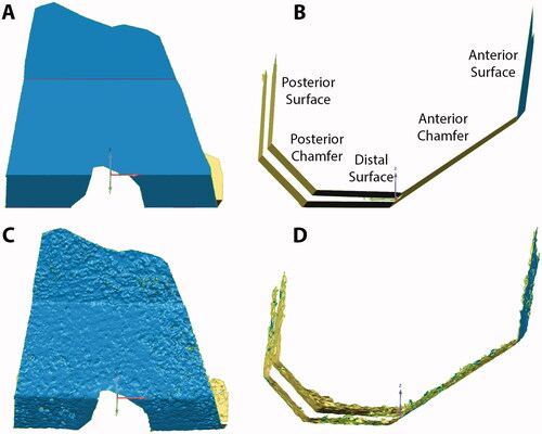
One surgeon performed TKA on four fresh-frozen healthy cadaveric knees from four specimens using an active robotic system (TSolution One^® Total Knee Application, THINK Surgical^® Fremont, CA) [25]. Preoperative CT scans were imported into a CT-based pre-operative planning software (TPLAN^®) in which a three-dimensional (3D) bone model of the knee is generated. Next, the surgeon virtually selects the ideal size and placement of the tibial and femoral components, which generates nominal cut surfaces on the bone models resulting from the nominal geometry of the implant (Figure 1). Intra-operatively, a standard medial parapatellar approach was used to expose the knee joint. Next, the leg was rigidly attached to the active robot (TCAT^®) via fixation pins, and registration recovery markers were placed in the tibia and femur. Landmark registration was performed to inform the robot of the knee's position in space and to confirm the robot's ability to execute the preoperative plan. Next, the robot performed femoral and tibial cuts sequentially using a high-speed burr along a defined cut path. The robot was then removed from the operative field and the surgeon completed the procedure by removing marginal bone.

Figure 1. Nominal cut surfaces for a femur are shown in coronal (A) and sagittal (B) views. The names of the five femoral cut planes are also shown. The laser scanned cut surfaces of the same femur are also shown in coronal (C) and sagittal (D) views.

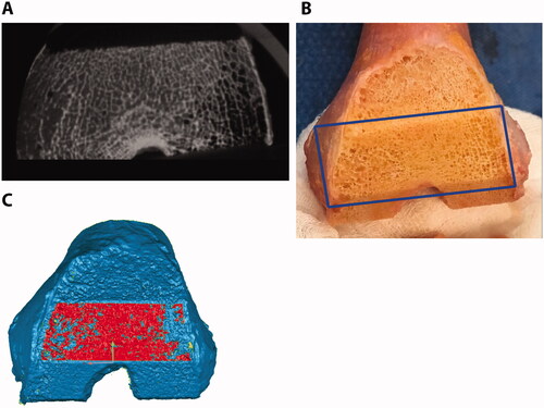
The resulting cut surfaces of the femur and tibia were optically scanned using a previously validated high accuracy laser scanner [26] (Metrascan 3D, Creaform, Canada) to generate the corresponding 3D models used for the analysis The laser scanner has a repeatability error of an 80 µm as measured in multiple scans of the same bone and overall accuracy of 83 µm as measured on a ceramic gage block. To reduce the reflectivity of the bone surface before laser scanning, the bones were wiped and left to air-dry for at least 30 min. Additionally, two commercially available femoral components of the same design were laser scanned after coating the surface with a thin layer of spray powder and one was implanted on one knee after laser scanning for a qualitative assessment of flatness after impaction. The resulting 3D models of the femur and tibia were used to determine the discrepancy in the topography between the nominal and the actual cut surfaces as a measure of the dimensional cutting accuracy of the active robotic system. Only areas cut by the robot were included in the analysis. Also, areas of high porosity in the cancellous bone, where little implant contact with trabeculae would have been possible, were excluded as the laser scanner would scan areas below the cut surface. To identify the regions for the analysis that exclude high bone porosities, each cut surface was selected based on a crease angle using Geomagic Control (3D Systems Inc., Rock Hill, SC, USA), which selects only contiguous polygons whose shared edges meet at a relatively low angle that can be user-defined [i.e. crease angle (Figure 2)]. Since there is subjectivity in the selection of the appropriate crease angle, each surface selection was verified by using micro-CTs to ensure only the high porosity regions were removed. Micro-CTs were collected (Quantun FX, Perkin Elmer, tube voltage of 90 kVp, tube current 180 μA, and a field-of-view of 75 mm which resulted in ∼148 μm slices) and resliced to align the image view to the cut surface that was being analyzed using Mimics^® (Materialise, Belgium). Regions with a lack of trabeculae that would cover a significant amount of surface were identified as high-porous regions (Figure 3). If the assessment done with micro-CT did not confirm the region selection in Geomagic Control, the crease angle was adjusted until a good match could be achieved. If available, gross photography was also used to confirm the match. Crease angles ranging from 8 to 17° and 10 to 19° were selected for the femur and tibial cut surfaces, respectively.

Figure 2. Femoral cut surfaces were selected (red) based on crease angles of 15° (A), 20° (B), and 25° (C). As the crease angle is increased, more porous regions are selected.

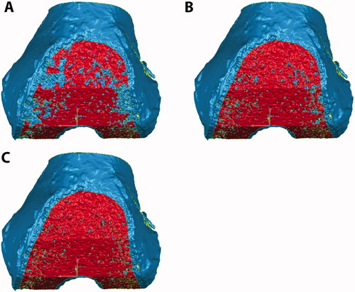
Figure 3. Micro-CT (A), gross photography (B), and laser scan (C) show the same femoral anterior chamfer cut surface for one representative specimen. Dark regions in the micro-CT are porous regions that are not densely occupied by trabeculae. An appropriate crease angle was used to select the cut bone surface (red) in the laser scan without significant trabecular porosity.

Planes were best-fit to each of the femoral and tibial cut surfaces and flatness was computed as the standard deviation between the cut surface and the best-fit plane [17] (Figure 4). For the femoral cut surfaces, the angles between each of the best-fit planes and the other four planes were compared to the nominal values via a pairwise comparison for a total of twenty angular differences (Figure 5). The mean and standard deviation of the five errors for each cut plane was then calculated. To compare the bone cutting error to the manufacturing error of the implant, an additional angular analysis was done on the implant. Specifically, the angular errors were computed for the two femoral components by comparing the 3D geometry of the five cut planes from the laser-scanned implants to the ones from the nominal implant CAD geometry. Additionally, the normal point-to-point distances between each of the five femoral cut surfaces on the bone to the respective nominal cut planes were computed. This was accomplished by shape-matching the entire femoral cut surfaces (i.e. inclusive of the five cut surfaces) to the entire nominal femoral cut surfaces using the iterative closest point algorithm implemented in Geomagic Control. This distance provides an overall measure that takes into account errors in cut surface flatness, length, and orientation. The resulting distances were analyzed with 3D deviation maps to determine what percentage of the cut surface has a <1 mm gap from the nominal cut surfaces, thus serving as an estimate of the bone-to-implant gap (Figure 6). Means and standard deviations were calculated for all measurements after confirming that the measurements were normally distributed.

Figure 4. Deviation maps show the distance between each cut surface and the best-fit plane. The best-fit plane was created without including the boundaries of the surface to avoid regions where the surgeon manually removed marginal bone. Flatness was computed as the standard deviation of the distance between the cut surface and the best-fit plane. Scale is in mm.

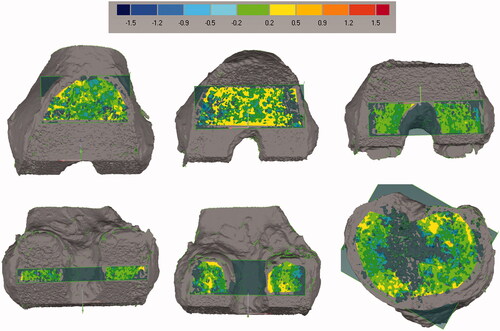
Figure 5. Steps for computing femoral cut plane angular errors. Planes were best-fit to each cut surface. The angle between each cut plane and all other cut planes, even non-adjacent ones, was calculated for a total of twenty angular differences for each femur. The figure shows the four angles that were calculated for the anterior chamfer (A) and distal surface (B). Similar measurements were made for the other three surfaces. The twenty angle errors were computed by subtracting the nominal angles from the measured angles. This measurement was not performed for the tibia given it only has one planar cut.

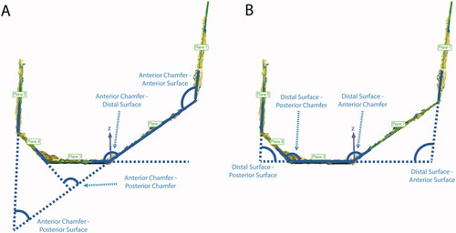
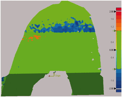
Figure 6. Steps for computing distance errors for the femoral cuts from the nominal cut planes. All five cut surfaces were shape matched to the nominal cut planes. A 3D deviation map was then computed to determine which percentage of the cut surface was within the tolerance of ±1 mm. Green colors indicate that the surface was within tolerance, while red and blue colors indicate that the actual cut was too far outside and inside the planned cut, respectively.

Lastly, a qualitative analysis of the cut surfaces was also performed to visually assess flatness using microradiographs (Figure 7) and to determine the rate of smooth vs. frayed trabeculae with scanning electron microscopy (SEM) (Figure 8) on two knees (i.e. one with implant and one without implant).

Figure 7. Microradiographs of a sagittal section of the femur (A) and coronal section of the tibia (B), show the flatness of each cut. Arrows point to portions of bone that were uncut as a result of the chosen preoperative plan and would be outside of where the implant would rest and were not analyzed. To create the microradiographs, the bones were fixed in 10% Neutral Buffered Formalin, dehydrated in ascending grades of ethanol, infiltrated, and embedded in polymethyl methacrylate. Once the specimens were polymerized, 2 mm thick sections were made from each polymerized block. High-resolution contact radiographs were then made of each section.

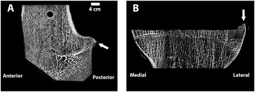
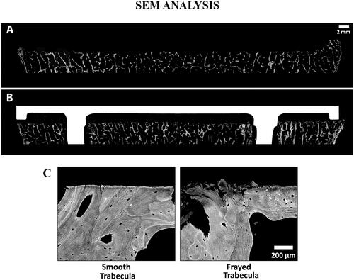
Figure 8. SEM images of a tibia without an implant (A) and a different tibia with cemented implant (B), with Gray = Bone, White = Implant, and Black = Soft Tissue/Cement. The cut surface is noticeably flattered on the specimen that has an implant. Comparison of a smooth vs. frayed trabecula (C) from SEM image. For the femur with an implant, the ratio of smooth vs. frayed trabecular was similar to the femur without an implant (67 vs. 68% smooth trabeculae), but for the tibia, the one with an implant had a higher amount of smooth trabeculae (37 vs. 47%). To create the SEM images, one section from each specimen was ground and polished to an optical finish. The polished ∼2 mm-thick sections were coated with a thin conductive layer of carbon for ∼25 s and imaged using a JEOL JSM-6610 SEM equipped with a backscatter electron (BSE) detector and associated imaging software. Digital BSE images were captured along the entire resected surface and then stitched together for (A) and (B).

Results

The cut surfaces had an average flatness of 0.16 ± 0.06 mm (Mean ± STD) with low variability between different cut planes with flatness ranging from 0.11 ± 0.04 mm for the femoral distal surface to 0.23 ± 0.07 mm for the femoral posterior surface (Table 1). The femoral cut surfaces had average angular errors of 0.47 ± 0.39°, ranging from 0.35 ± 0.35° for the anterior chamfer to 0.55 ± 0.41° for the posterior chamfer (Table 2). These angular errors are of similar magnitude as the ones found for the implants, which vary from 0.23 ± 0.10° for the anterior chamfer to 0.45 ± 0.19° for the posterior chamfer. The bone-to-implant gap, estimated with the deviations between the five femoral cut surfaces to the nominal cut planes, was within ±1 mm for 97.9% of the surface on average, ranging from 94.2% for the posterior surface to 100% for the distal surface and posterior chamfer (Table 3). From a qualitative standpoint, cross-sectional radiographs showed that cut surfaces were flat in all cut planes (Figure 7). From the SEM analysis, it was found that the femur had 67–68% smooth vs. 33–31% of frayed trabeculae while the tibia had 37–47% smooth vs. 63–32% frayed trabeculae (Figure 8).

Table 1. Flatness errors (mean ± standard deviation, range) for the femoral and tibial cut surfaces (mm).

	Cut surfaces
Anterior surface	0.18 ± 0.02, 0.16–0.20
Anterior chamfer	0.13 ± 0.04, 0.09–0.18
Distal surface	0.11 ± 0.03, 0.09–0.17
Posterior chamfer	0.13 ± 0.02, 0.11–0.15
Posterior surface	0.23 ± 0.07, 0.16–0.32
Tibial surface	0.20 ± 0.02, 0.18–0.22
Overall average	0.16 ± 0.06, 0.09–0.32

Table 2. Angular errors (mean ± standard deviation) for both the femoral cuts and implants (degrees).

	Femur cuts	Implants
Anterior surface	0.48 ± 0.38	0.23 ± 0.10
Anterior chamfer	0.35 ± 0.35	0.25 ± 0.20
Distal surface	0.41 ± 0.43	0.24 ± 0.19
Posterior chamfer	0.55 ± 0.41	0.29 ± 0.22
Posterior surface	0.54 ± 0.39	0.45 ± 0.19
Overall	0.47 ± 0.39	0.29 ± 0.19

Table 3. Percentage of the femoral cut surfaces that would have a <1 mm bone-implant gap.

Cut surface	Percentage of cut surface within 1 mm
Anterior surface	94.5%
Anterior chamfer	99.6%
Distal surface	100.0%
Posterior chamfer	100.0%
Posterior surface	94.2%
Overall	97.9%

Discussion

The current study describes a novel methodology used to compute the dimensional cutting accuracy of both the femoral and tibial bone cuts of an active robotic system that uses a high-speed burr for TKA. The first main finding was that the measurement technique implemented in this study allowed to measure the angular errors and to estimate the bone-to-implant gap in the femoral cuts in addition to femoral and tibial cut flatness. The second main finding was that a high dimensional accuracy was found for both femoral and tibial cuts, with 97.9% of the femoral cut surface was found to be within the 1 mm gap from the nominal surface, which has been previously shown to be necessary for bony ingrowth [24], with angular errors of similar magnitude to the manufacturing errors found in commercially available femoral implants, and with high flatness for both the femoral and tibial cuts.

The measurement technique implemented in this study allowed for the first time to quantify the dimensional accuracy of the femoral cuts by determining the relative angular error between the five cut planes and by estimating the bone-to-implant gap as deviation errors from the nominal surface. The technique allowed for the proper exclusion of the porosities present in the cancellous bone using a methodology based on a ‘crease angle’ and verification via micro-CT. However, the authors believe that using good-quality photographs of each cut plane could have been sufficient to verify that porous surfaces were excluded.

While there is limited research into the dimensional accuracy of TKA cut surfaces with which the results of the present study can be compared, there has been some research into cut surface flatness for the tibia. The average tibial cut surface flatness of 0.20 mm found in the present study is better and the flatness range is narrower [0.16–0.22 mm] than the flatness found in two studies by Toksvig-Larsen et al. with manual instruments which reported an average flatness of 0.26 mm18 and 0.49 mm19 with flatness ranges of [0.16–0.38 mm] and [0.30–0.68 mm], respectively. Delgadillo et al. found the flatness of tibial cut surfaces using conventional instruments to be 1.1 ± 0.35 mm16, however, a different methodology for calculating flatness was used so the results could not be compared directly to the ones of this study. Specifically, their methodology involved finding the height of the zone above and below the plane of best-fit that encompassed 99% of the surface volume. Both Toksvig-Larsen et al. and Delgadillo et al. found a depression in the center of the tibial plateau, which is theorized to be caused by the oscillating saw blade cutting less cleanly through the softer cancellous bone that is present in that region. Microradiographs from the present study showed that the robotic system created a flat tibial cut without depression in the center of the plateau (Figure 7). Previous studies using a robotic arm with a burr to cut a tibial surface found similar results as the present study, with flatness ranging from 0.15 to 0.29 mm [20,21]. Lastly, it needs to be noted that during impaction, viscoelastic deformation of the bone may occur which may damage the bone and affect dimensional accuracy. However, previous research has found that the flatness of the tibial surface will further improve when the implant is impacted on the bone [16], which was also visible in SEM imaging in the present study (Figure 8).

There are some limitations to the present study, none of which has a major influence on the results or conclusions. The study did not include an analysis for a manual control group, which would have made it possible to directly compare the dimensional accuracy of TKA surfaces prepared using the robotic system to TKA surfaces prepared using standard manual instrumentation. However, it was possible to compare the tibial cut surface flatness to results from previous studies to the extent possible. Only one surgeon participated in this study as the dimensional accuracy is independent of the specific user. However, the participation of multiple surgeons could have increased the reliability of the measuring technique and confirmed the generalizability of these results to a broader surgeon population. The bone-to-implant distance was estimated by determining the distance between the actual cut surface and the nominal cut surface after a shape-match, which may be different from how an implant would press fit onto the cut surface. However, differences should be relatively small for the cut surfaces in this study because they were found to have high dimensional accuracy. Regions of high bone porosity had to be removed from the 3D models of the cut surfaces because they did not reflect the flatness of the surfaces as cut by the robot. While these removed regions were relatively small, a new technique would be needed to measure the entire cut surface. The flatness of the cut surfaces was measured without impacting an implant onto the bone, which is a process that may change surface flatness. Previous research has found that this should only improve results, with the flatness of the tibial surface improving after the implant was impacted onto the bone [16]. Lastly, new techniques for measurement of accuracy may require validation by other studies and comparisons to previously used techniques.

Further research is needed to explore dimensional accuracy in TKA. In cemented TKA, it is unclear what level of dimensional accuracy is required to ensure fixation of the implant because the cement fills most of the gaps and thus ensures good conformity between the bony and implant surfaces. The required dimensional accuracy in cementless TKA is likely higher because any large gaps will inhibit bony ingrowth. Clinical studies determining the effect of dimensional accuracy on TKA success for both cemented and cementless TKA are needed to determine acceptable tolerances. Lastly, studies exploring the dimensional accuracy of the femoral as well as the tibial bone cuts of other commercially available robotic systems are needed, along with comparisons of the dimensional accuracy for conventional and robotic techniques.

Conclusion

The study describes a novel methodology used to compute the dimensional cutting accuracy of an active robotic system that uses a high-speed burr for TKA. This methodology allowed us to determine for the first time the dimensional accuracy of the femoral cuts in addition to the tibial cuts and found high accuracy for the active system, with 97.9% of the femoral surface being within the 1 mm bone-to-implant distance necessary for bony ingrowth, with angular errors of similar magnitude to the manufacturing errors found in commercially available femoral implants, and with high flatness for both the femoral and tibial cuts.

Disclosure statement

Stefan Kreuzer has received research support, is a paid consultant, and has done paid presentations for THINK Surgical^®. Abheetinder Brar and Valentina Campanelli are paid employees of THINK Surgical.

References

- Kuzyk PRT, Schemitsch EH. The basic science of peri-implant bone healing. Indian J Orthop. 2011;45(2):41–115.
- Cho Y, Lee MC. Rotational alignment in total knee arthroplasty. Asia Pac J Sport Med Arthrosc Rehabil Technol. 2014;1(4):113–118.
- Longstaff LM, Sloan K, Stamp N, et al. Good alignment after total knee arthroplasty leads to faster rehabilitation and better function. J Arthroplasty. 2009;24(4):570–578.
- Barrack RL, Schrader T, Bertot AJ, et al. Component rotation and anterior knee pain after total knee arthroplasty. Clin Orthop Relat Res. 2001;392:46–55.
- Berger RA, Crossett LS, Jacobs JJ, et al. Malrotation causing patellofemoral complications after total knee arthroplasty. Clin Orthop Relat Res. 1998;356:144–153.
- Lonner JH, Fillingham YA. Pros and cons: a balanced view of robotics in knee arthroplasty. J Arthroplasty. 2018;33(7):2007–2013.
- Kayani B, Konan S, Ayuob A, et al. Robotic technology in total knee arthroplasty: a systematic review. EFORT Open Rev. 2019;4(10):611–617.
- Parratte S, Price AJ, Jeys LM, et al. Accuracy of a new robotically assisted technique for total knee arthroplasty: a cadaveric study. J Arthroplasty. 2019;34(11):2799–2803.
- Sires JD, Craik JD, Wilson CJ. Accuracy of bone resection in MAKO total knee robotic-assisted surgery. J Knee Surg. 2021;34(7):745–748.
- Hampp EL, Chughtai M, Scholl LY, et al. Robotic-arm assisted total knee arthroplasty demonstrated greater accuracy and precision to plan compared with manual techniques. J Knee Surg. 2019;32(3):239–250.
- Angibaud LD, Dai Y, Liebelt RA, et al. Evaluation of the accuracy and precision of a next generation computer-assisted surgical system. Clin Orthop Surg. 2015;7(2):225–233.
- Mont M, Kinsey T, Zhang J, et al. Robotic assisted total knee arthroplasty demonstrates greater component placement accuracy compared to manual instrumentation: initial results of a prospective multi-center evaluation. Int Soc Technol Arthroplast. 2019;102:2019–2021.
- Seidenstein A, Birmingham M, Foran J, et al. Better accuracy and reproducibility of a new robotically-assisted system for total knee arthroplasty compared to conventional instrumentation: a cadaveric study. Knee Surg Sport Traumatol Arthrosc. 2020;29:859–866.
- Casper M, Mitra R, Khare R, et al. Accuracy assessment of a novel image-free handheld robot for total knee arthroplasty in a cadaveric study. Comput Assist Surg. 2018;23(1):14–20.
- Koulalis D, O'Loughlin PF, Plaskos C, et al. Sequential versus automated cutting guides in computer-assisted total knee arthroplasty. Knee. 2011;18(6):436–442.
- Delgadillo LE, Jones HL, Ismaily SK, et al. How flat is the tibial osteotomy in total knee arthroplasty? J Arthroplasty. 2019;35(3):870–876.
- Toksvig-Larsen S, Ryd L. Surface flatness after bone cutting. A cadaver study of tibial condyles. Acta Orthop Scand. 1991;62(1):15–18.
- Toksvig-Larsen S, Ryd L. Surface characteristics following tibial preparation during total knee arthroplasty. J Arthroplasty. 1994;9(1):63–66.
- Toksvig-larsen S, Kroon PO, Ryd L. Improved bone cutting using a semirotating saw. A cadaver study of the cut surface on tibial condyles. Acta Orthop Scand. 1994;65(4):412–414.
- Van Ham G, Denis K, Vander Sloten J, et al. Machining and accuracy studies for a tibial knee implant using a force-controlled robot. Comput Aided Surg. 1998;3(3):123–133.
- Denis K, Van Ham G, Vander Sloten J, et al. Influence of bone milling parameters on the temperature rise, milling forces and surface flatness in view of robot-assisted total knee arthroplasty. Int Congr Ser. 2001;1230(C):300–306.
- Witmer DK, Meneghini RM. Cementless total knee arthroplasty: patient selection and surgical techniques to optimize outcomes. Semin Arthroplasty. 2018;29(1):50–54.
- Kayani B, Konan S, Pietrzak JRT, et al. Iatrogenic bone and soft tissue trauma in robotic-arm assisted total knee arthroplasty compared with conventional jig-based total knee arthroplasty: a prospective cohort study and validation of a new classification system. J Arthroplasty. 2018;33(8):2496–2501.
- Dalton JE, Cook SD, Thomas KA, et al. The effect of operative fit and hydroxyapatite coating on the mechanical and biological response to porous implants. J Bone Joint Surg Am. 1995;77(1):97–110.
- Chan J. Active robotic total knee arthroplasty (TKA): initial experience with the TSolution One® TKA System; 2020.
- Campanelli V, Howell SM, Hull ML. Accuracy evaluation of a lower-cost and four higher-cost laser scanners. J Biomech. 2016;49(1):127–131.