An automated optimization pipeline for clinical-grade computer-assisted planning of high tibial osteotomies under consideration of weight-bearing

Abstract

3D preoperative planning for high tibial osteotomies (HTO) has increasingly replaced 2D planning but is complex, time-consuming and therefore expensive. Several interdependent clinical objectives and constraints have to be considered, which often requires multiple rounds of revisions between surgeons and biomedical engineers. We therefore developed an automated preoperative planning pipeline, which takes imaging data as an input to generate a ready-to-use, patient-specific planning solution. Deep-learning based segmentation and landmark localization was used to enable the fully automated 3D lower limb deformity assessment. A 2D-3D registration algorithm allowed the transformation of the 3D bone models into the weight-bearing state. Finally, an optimization framework was implemented to generate ready-to use preoperative plannings in a fully automated fashion, using a genetic algorithm to solve the multi-objective optimization (MOO) problem based on several clinical requirements and constraints. The entire pipeline was evaluated on a large clinical dataset of 53 patient cases who previously underwent a medial opening-wedge HTO. The pipeline was used to automatically generate preoperative solutions for these patients. Five experts blindly compared the automatically generated solutions to the previously generated manual plannings. The overall mean rating for the algorithm-generated solutions was better than for the manual solutions. In 90% of all comparisons, they were considered to be equally good or better than the manual solution. The combined use of deep learning approaches, registration methods and MOO can reliably produce ready-to-use preoperative solutions that significantly reduce human workload and related health costs.

Keywords:

• 3D surgical planning
• automatic
• high tibial osteotomy
• multi-objective optimization

1. Introduction

Opening wedge high tibial osteotomy (OWHTO) is a surgical procedure which aims to realign the lower limb to shift the load from the damaged medial compartment of the knee to the healthy lateral compartment in patients with symptomatic osteoarthritis (OA) associated with a genu varum deformity [1]. However, a precise anatomical correction is crucial since over- and undercorrection are known to be the main reasons for clinical failure [2,3]. For instance, unintended changes of the tibial slope (TS) [4] or tibial tuberosity can result in anteroposterior instability and increased strain on the cruciate ligaments [5–7] or alteration of patellofemoral tracking [8]. Strategic preoperative planning is thus a crucial element of clinical success. Traditionally, 2D long-leg standing radiographs are used, taking the mechanical axis (MA) as the most important parameter. For the past decades, the principles published by Paley et al. [9] have been widely used as the general guideline in this regard. With the emergence of modern computer-assisted techniques, 2D preoperative planning based on radiographs has gradually been replaced by methods using Computer Tomography (CT)-reconstructed 3D bone models. The latter not only provides the surgeon with the detailed patient anatomy, but also allows for preoperative 3D measurements [10] and treatment planning [11], biomechanical simulations [12] and the use of patient-specific instruments (PSI) [13]. Furthermore, 3D approaches enable computer-assisted interventions (CAI) based on navigation [14] or robotics [15]. However, state-of-the-art 3D preoperative planning has its shortcomings: although automatic planning approaches have been proposed [16], these still requires the manual generation of preoperative planning solutions by trained interdisciplinary teams [17,18], which makes the entire process expensive and time-consuming. Due to additional degrees of freedom (DoF) and added complexity in 3D, the planning process is not only tedious but also technically demanding. Therefore, the close collaboration of surgeons and engineers is required throughout the planning process to combine technical with clinical and surgical knowledge. The integration of the combined knowledge into computer algorithms is the main obstacle to overcome during the development of automated computer methods for preoperative planning; a compromise between automation and adaptability has to be found.

Our work aimed to achieve this balance by developing the first fully automated pipeline for clinical-grade preoperative OWHTO planning, one that is compatible with use in the clinical setting while maintaining the ability to tailor the solutions to the individual patient. With only the input of medical images, our pipeline generates ready-to-use preoperative solutions. In two evaluation rounds with medical experts, we optimized our algorithm to ensure not only technical feasibility but also the incorporation of all their clinical expertise. The main contributions of our work are:

• Fully automated deformity assessment of the lower limb in 3D: fully convolutional neural networks (FCNN) are used for both segmentation of all bones and landmark localization in CT scans. Mechanical axis (MA) as well as tibial slope (TS) are automatically measured from imaging data, no manual annotations are required.

• Introducing 3D planning under weight-bearing conditions based on a fully automated 2D-3D registration approach [19]

• The implementation of a multi-objective optimization algorithm (MOO), including the development of planning objective functions to find the best tradeoff solution for the optimization of osteotomies of the lower limb.

The pipeline was finally evaluated with five medical experts, based on 53 real patient cases. The experts blindly rated and commented the automatically generated as well as the manually planned preoperative solution.

1.1. Related work

1.1.1. Automated preoperative planning

Only few works have focused on automated planning of long-bone corrective osteotomies so far. Fifteen years after the work of Eck et al. [20] on proximal femur corrections, Schkommodau and Belei [21,22] developed an automatized multi-objective optimization strategy for planning corrective osteotomies of lower extremities. They solved a 12 DoF optimization problem by including parameters for the osteotomy, leg length, angulation, translation and antetorsion, but did not consider the placement of the fixation plate and screws. Their method was based on sequential quadratic programming [23] for finding the optimal solution, but instead of patient-specific anatomies, they used simplified geometrical models that were calibrated based on intraoperatively acquired radiographs. Although the approach was evaluated using plastic bones under idealized laboratory conditions, the obtained accuracy was not yet sufficient for clinical implementation. Nevertheless, their work pioneered the field and proved general feasibility of the approach.

Most recently, our group used a genetic algorithm to generate ready-to-use 3D preoperative planning solutions for osteotomies in the forearm in a fully automated fashion [17,24]. Position and orientation of the osteotomy plane, the required transformation to achieve bone reduction as well as the position and orientation of the fixation plate and screws were automatically optimized. The proposed solutions were evaluated and compared to the manually planned gold-standard solutions by experienced surgeons and engineers, whereby they assessed the automatic solutions to be better in 55% of the cases. Even in the remaining 45%, the quantitative evaluation showed only minor deviations from the gold standard [24]. A similar algorithm was used to optimize the three-dimensional (3D) positioning of pedicle screws for spinal fusion surgery to achieve mechanically robust inserted screws based on the CT-derived bone properties [25]. The method was validated using cadaver lumbar vertebrae, resulting in a 26% increased pull-out strength for the screws with optimized trajectories and sizes. Particle swarm optimization, another nature inspired optimization algorithm, was successfully used to plan bone tumor resections and minimize the collaterally resected healthy bone [26].

Besides optimization algorithms, machine learning approaches have been used to automate certain steps in preoperative planning. Lambrechts and colleagues [27] trained non-linear regression models to predict corrections a surgeon would make to a manufacturer’s default preoperative plan for total knee arthroplasties (TKA). Yue et al. [28] used radiographs as well as relevant physical features as input for deep learning (DL) models for preoperative prediction of the best prosthetic type in TKA. Similarly, in shoulder arthroplasty, the location and orientation of the articular marginal plane (AMP) has been estimated using either random regression forests [29] or DL [30], both only relying on a CT scan as input. In our group, deep reinforcement learning has been successfully used to find the two cutting planes which are required to obtain a spherical femoral head in femoral head reduction osteotomies (FHRO) [31]. While the latter does not require patient data for training, (supervised) DL approaches are often limited by the respective training data sets. With increasing complexity (constraints) and DoF, a larger training data set is needed to guarantee generalizability. Additionally, the integration of user feedback is challenging in DL approaches.

Given the variety of constraints and degrees of freedom of an HTO procedure and the recent successful use of genetic MOO algorithms for similar tasks, we chose to employ the same approach for our problem. The major contributions here are the design of objective functions and the formulation of the constraints as well as the hyperparameter definition.

1.1.2. Registration

2D-3D image registration is a large and active research field [32–35], but the use of 2D-3D registration for CAI planning of corrective osteotomies has only rarely been adressed in the literature. Despite the importance of joint loading in the etiology of osteoarthritis and the repeatedly reported differences in alignment between loaded and unloaded states [10,36,37], 3D imaging data in a weight-bearing state [38] is usually not available. Kobayashi first registered lower extremity 3D models to two standing radiographs by minimizing the difference between the projected outline of the 3D models and the contour in the radiographs [39]. We implemented an intensity-based registration algorithm to register the non-weight-bearing CT scans to standing radiographs.

1.1.3. Landmark localization

Various approaches have been published for landmark localization, such as direct coordinate regression [30] or displacement vector prediction [40]. However, this involves a highly non-linear mapping between image features and point or vector coordinates. In contrast, heatmap representations of landmark coordinates, encoding the pixel-wise probability distribution for one particular landmark, are more closely associated with the input image. In extensive works, Payer et al. [41,42] employed a FCNN architecture which learns the spatial configuration of multiple landmarks and their local appearance in two separate parts of the same network. The precision of their results was varying between image modalities (CT, MRI, radiographs), anatomies (hand, spine, skull) and dimensionalities (2D and 3D). To the best of our knowledge, the work of Zhao et al. [43] is the only one localizing lower limb landmarks in CT scans. They used the same principle as Payer [42] but trained two spatial configuration networks in series, one for the coarse localization on downscaled images and one for the fine localization on high resolution patches that were tightly cropped around the coarsely localized coordinates. They localized six different landmarks in knee CT scans, one of them being the knee joint center and reported a mean error of 1.3 mm across all six localized landmarks. The error for the individual landmarks were not reported. Similarly, we used heatmap regression based FCNN to automatically localize hip, knee and ankle joint centers (HJC, KJC, AJC) in CT scans.

2. Methods

Our proposed optimization pipeline for the automatic planning of OWHTO procedures is depicted in Figure 1. It is composed of three different modules: deformity assessment (module 1, including segmentation, deep-learning based landmark localization and deformity measurement), 2D-3D registration for weight-bearing transformation (module 2) and intervention planning (module 3). The input for the pipeline is an imaging dataset consisting of a CT scan and a biplanar long-leg standing radiograph, which is also the current standard in our clinic. As an output, it provides a ready-to-use preoperative planning solution including STL models of all bones (femur $\mathit{F},$ tibia $\mathit{T},$ fibula $\mathit{FB}$ and patella $\mathit{P}$) as well as the position and orientation of (1) the osteotomy axis, (2) the osteotomy plane and (3) the fixation plate.

Figure 1. Pipeline overview. The proposed pipeline consists of 3 modules: First, the deformed bones are automatically segmented from the CT scan to measure the deformity using DL-based landmark localization (M1). Second, the CT is registered to the biplanar long-leg standing radiographs to transform the 3D models into a weight-bearing state (M2). Finally, a multi-objective optimization algorithm is used (M3) to automatically find a preoperative solution and place the osteotomy axis, cutting plane and fixation plate, including screws.

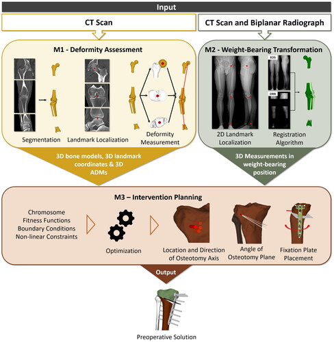
Each of the above-mentioned modules addresses specific issues of the current clinical pipeline. Module 1 uses a FCNN to fully automate the segmentation of all bones from the input CT scan, which is currently done manually. Furthermore, it automates deformity analysis by using another FCNN to predict all required landmarks from the CT and calculate the preoperative anatomical deformity measurements (ADM). Module 2 enables the transformation of 3D models and the respective landmarks to the weight-bearing state by employing an intensity-based algorithm for 2D-3D registration between CT and biplanar standing radiographs (EOS imaging system, EOS, Paris, France). Module 3 addresses the tedious and difficult process of manual osteotomy planning by implementing a variant of NSGA-II [44], which is the state-of-the-art in multi-objective genetic algorithms, to automatically find the ideal osteotomy parameters while considering all clinical constraints.

2.1. Manual 3D deformity assessment

Prior to surgery, the bone deformity for each patient must be measured to quantify the required surgical correction. Currently, this 3D preoperative deformity assessment is performed manually, including three major steps: segmentation of the 3D bone models from the CT scan, annotation of all required landmarks using the segmented 3D bone models and subsequent assessment of the ADMs. Using these manual methods, we generated the ground truth data which is required to train the networks for the automated methods described in section Module 1 - Automated 3D deformity assessment.

The segmentations were performed semi-automatically using commercial segmentation software (Mimics Medical 19.0, Materialize NV, Leuven, Belgium). 3D models were generated using the Marching Cube algorithm [45] and were represented in the form of triangular surface meshes (stereolithographic models; STL) as described by Roscoe et al. [46].

The 3D models were imported in our in-house planning software CASPA (CASPA 5.32, University Hospital Balgrist, Zurich, Switzerland), where all the landmarks were annotated and the measurements performed as summarized in Table 1 and shown in Figure 2.

Figure 2. Manual annotation methods, as used for the ground truth annotations. (A) Alignment of the 3D models in the planning coordinate system with its frontal (brown), sagittal (gree) and axial (beige) plane. (B) Manual determination of $H_C^{3D},$ $K_C^{3D}$ and $A_C^{3D}$ in 3D. (C) The slope plane normal vector ${\overrightarrow{n}}_S$ is determined by fitting a plane to manually selected points on the tibial plateau. (D) The MA is defined by the angle α between ${\overrightarrow{a}}_F$ and ${\overrightarrow{a}}_T.$ (E) The TS is defined as 180° - β, with β as the angle between ${\overrightarrow{a}}_T$ and ${\overrightarrow{n}}_S.$

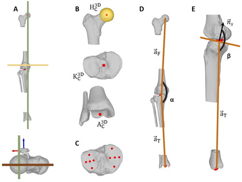
Table 1. Overview of the landmarks required for deformity assessment including their determination in manual and automated planning.

Name	Symbol	Manual definition
Hip Joint Center	$H_C^{3D}$	Center of a sphere fitted to user selected points of the femoral head [11]
Knee Joint Center	$K_C^{3D}$	Midpoint between the two tibial eminences [11]
Ankle Joint Center	$A_C^{3D}$	Center of all points on the tibial & fibular articular surface, which are defined by calculating the closest-point distance to the talus and subsequently only consider points below a user defined distance threshold [11]
Tibial Slope Plane Normal	${\overrightarrow{n}}_S$	Fitting of a plane through user selected points on the tibial plateau [11]
Patella Normal	${\overrightarrow{n}}_P$	3^rd component of PCA of patella 3D model [47]

In a first step, the hip joint center, $H_C^{3D}\in {\mathbb{R}}^3,$ the knee joint center, $K_C^{3D}\in {\mathbb{R}}^3$ and the ankle joint center $A_C^{3D}\in {\mathbb{R}}^3$ were determined using the methods given in Table 1 (Figure 2(B)). Subsequently, the 3D models were transformed into the planning coordinate frame representing anatomical planes: the positive x, y and z axes correspond to the left, superior and anterior directions. To this end, the connecting line between ${\mathrm{A}}_{\mathrm{C}}^{3\mathrm{D}}$ and ${\mathrm{H}}_{\mathrm{C}}^{3\mathrm{D}}$ was aligned with the y-axis of the coordinate system. Principal component analysis (PCA) [47] was applied to the patella and the third principal axis ${\overrightarrow{n}}_P$ was used to orient the models in the axial plane by aligning ${\overrightarrow{n}}_P$ with the z-axis of the planning coordinate frame (Figure 2(A)). Once oriented, the femoral and tibial mechanical axes (${\overrightarrow{\mathrm{a}}}_{\mathrm{F}},$ ${\overrightarrow{\mathrm{a}}}_T$) were defined as the lines connecting the $H_C^{3D}$ with the $K_C^{3D}$ and the $K_C^{3D}$ with the $A_C^{3D}$ (Equation (1)(1) $${\overrightarrow{a}}_F=\mathrm{ }{K}_C^{3D}\text{-}\mathrm{ }{H}_C^{3D}$$(1) and Equation (2)(2) $${\overrightarrow{a}}_T=\mathrm{ }{A}_C^{3D}\text{-}\mathrm{ }{K}_C^{3D}$$(2) , respectively). (1) $${\overrightarrow{a}}_F=\mathrm{ }{K}_C^{3D}\text{-}\mathrm{ }{H}_C^{3D}$$(1) (2) $${\overrightarrow{a}}_T=\mathrm{ }{A}_C^{3D}\text{-}\mathrm{ }{K}_C^{3D}$$(2)

The MA was finally defined as the angle between ${\overrightarrow{a}}_F$ and ${\overrightarrow{a}}_T$ (Figure 2(D)), projected to the frontal plane by projection matrix $P_F:$ (3) $$MA({\overrightarrow{a}}_F,\mathrm{ }{\overrightarrow{a}}_T)=\mathrm{ }{\mathit{tan}}^{-1}(\frac{\Vert P_F{\overrightarrow{a}}_F\mathrm{ }\times {P_F\overrightarrow{a}}_T\Vert }{{P_F\overrightarrow{a}}_F·{P_F\overrightarrow{a}}_T})$$(3)

The TS is defined by the angle between the tibial mechanical axis ${\overrightarrow{a}}_T\in {\mathbb{R}}^3$ and the normal to the tibial slope plane ${\overrightarrow{n}}_S\in {\mathbb{R}}^3,$ projected to the sagittal plane with projection matrix ${\mathrm{P}}_{\mathrm{S}}$ (Figure 2(E)). ${\overrightarrow{n}}_S$ was found by hyperplanar fitting of a plane to manually selected points on the tibial plateau using orthogonal regression (Figure 2(C)) [48]. (4) $$TS({\overrightarrow{a}}_T,\mathrm{ }{\overrightarrow{n}}_S)=\mathrm{ }{\mathit{tan}}^{-1}(180°\text{-}\mathrm{ }\frac{\Vert P_S{\overrightarrow{n}}_S\mathrm{ }\times {P_S\overrightarrow{a}}_T\Vert }{{P_S\overrightarrow{n}}_S·{P_S\overrightarrow{a}}_T})$$(4)

2.2. Module 1 - automated 3D deformity assessment

As an input, the module uses the CT scan of the patient’s lower-extremity. The output consists of the 3D bone models as well as the coordinates of all required orthopedic landmarks and the corresponding ADMs. Both for segmentation as well as landmark localization, we use a deep-learning approach based on U-net architectures [49], which consist of a multi-level contracting path to extract image features and a symmetric expanding path to enable precise localization of these features. On each level of the symmetric, u-shaped network, skip connections are used to combine the outputs of the contracting and the expanding path to form the input of the next convolutional layer in the expanding path.

The ground truth segmentation and landmark annotations were performed semi-automatically as described in section Manual 3D deformity assessment. The dataset consisted of patients who underwent a corrective osteotomy of the leg (see section Data).

2.2.1. Segmentation

Our segmentation network consists of three U-nets, which were trained for hip, knee and ankle joint CT scans to automatically segment the lower limb 3D bone models (femur $\mathit{F},$ tibia $\mathit{T},$ fibula $\mathit{FB}$ and patella $\mathit{P}$). Architecture as well as training details are summarized in Table 2 for a better overview, an example label map can be seen in Figure 3. Inspired by [50], we used a spatially weighted cross-entropy loss function for the segmentation networks to give more importance to the voxels in the surface area of a bones. The ground-truth label maps of the training samples were used to generate distance maps, where each voxel contained a value representing the distance to any bone surface. During training, the distance maps were applied for weighting the voxel-wise loss. Complete segmentations of all bones were obtained by fuzing the resulting label maps of the proximal and distal parts of each bone, and the evaluations of the segmentations were performed per bone.

Figure 3. Input and targets for segmentation and landmark localization networks. (A) Example for an input image (CT scan) of a proximal femur with its annotated HJC. (B) Target label map for the segmentaion U-net. (C) Target heatmap for the landmark localization U-net.

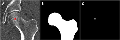
Table 2. Architecture and training details for the segmentation and landmark localization U-nets. The terms used in this table refer to the Tensorflow implementations for convolutional layers [51].

	Segmentation	Landmark localization
Input size	128 × 128 × 128 (hip, ankle) or 128 × 128 × 256 (knee)	128 × 128 × 128
Number of levels	5	5
Layers per level (encoding)	Conv > Conv > MaxPooling	Conv > Conv > MaxPooling
Layers per level (decoding)	UpSampling > Conv > Concatenate > Conv > Conv	UpSampling > Conv > Concatenate > Conv > Conv
Convolution kernel size	3 × 3×3×	3 × 3×3×
MaxPooling size	2 × 2×2	2 × 2×2
Filter numbers per level	32, 64, 128, 256, 512	32, 64, 128, 256, 512
Activation function	ReLu	ReLu
Padding	'same’	'same’
Weight initialization	He normal	He normal
Final layer activation function	Softmax	Sigmoid
Learning rate	1e-4	1e-4 (stage 1), 5e-5 (stage 2)
Optimizer	Adam	Adam
Loss function	Spatially weighted cross-entropy [50]	Binary cross-entropy
Epochs	50	30 (stage1), 60 (stage 2)
Batch size	1	1
Cross validation	5-fold	10-fold
Number of samples	115	116
Split of train/val samples	80% − 20%	80% − 20%

2.2.2. Landmark localization

Similarly, our localization network consists of three U-nets, one each for the localization of $H_C^{3D},$ $K_C^{3D}$ and $A_C^{3D}$ in the respective CT scans of hip, knee and ankle joints. The ground truth coordinate annotations were converted into heatmaps, which are images encoding the spatial probability of a landmark occurance at a certain voxel. The probability values were determined by applying a Gaussian distribution function around the ground truth coordinates of the landmarks, such that voxels near the ground truth location had the highest values, which then rapidly decreased with increasing distance. The heatmaps had the same dimensions as their corresponding medical image (e.g. a CT scan) and their values were normalized between 0 and 1. They were used as a learning target for the FCNN, which learned to reproduce them based on the input CT scan (Figure 3).

The U-net architecture as well as training details are described in Table 2. Briefly, a two-stage network was proposed to maximize accuracy of the joint center localization while optimizing GPU memory consumption. In the first stage, the original CT scans were downsampled to enable the processing of the entire CT. Candidate predictions were calculated from the output heatmaps and used for region-of-interest cropping of the high-resolution CT scans. The cropped, high-resolution images were then used as an input to the second stage.

2.2.2.1. Implementation details

The original CTs had a varying number of slices but a constant slice size of 512 × 512 pixels. In stage 1, the CTs were cropped or extended with zeros in the superior-inferior dimension, such that they all had a size of 512 × 512 × 512 voxels. The CTs were subsequently downsampled by factor 4, resulting in 128 × 128 × 128 voxels. Target heatmaps were generated using a Gaussian distribution around the annotated joint center coordinates and an empirically determined variance of 25 voxels across all dimensions.

For stage 2, the original CTs were cropped around the candidate predictions of stage 1 with a cubic crop size of 65, 60 and 60 mm for hip, knee and ankle joints, respectively. Prior to cropping, the cropping frame was translated randomly between 0 and 10 mm in all three directions to prevent that the landmark was always located around the center of the cropped image. The cropped images were then resampled to the dimensions of 128 × 128 × 128 voxels, resulting in resolutions of 0.51, 0.47 and 0.47 mm for hip, knee and ankle, respectively. The heatmaps were generated with an empirically determined variance of 4 across all dimensions. The center of all voxels containing a value greater or equal than 0.95 was calculated to find the landmark coordinates from the predicted heatmaps.

2.2.3. Deformity measurement

Based on the automatically localized landmarks, the MA was calculated as described in Equation (3)(3) $$MA({\overrightarrow{a}}_F,\mathrm{ }{\overrightarrow{a}}_T)=\mathrm{ }{\mathit{tan}}^{-1}(\frac{\Vert P_F{\overrightarrow{a}}_F\mathrm{ }\times {P_F\overrightarrow{a}}_T\Vert }{{P_F\overrightarrow{a}}_F·{P_F\overrightarrow{a}}_T})$$(3) . For the TS, the tibial slope plane was automatically found using a plane fitting algorithm of the Point Cloud Processing toolbox in Matlab (Matlab 2021a, The MathWorks Inc., Natick, MA, USA). The vertices in the most proximal 30 mm of the tibia bone model were isolated and a variant of the RANSAC algorithm [52] was employed to fit a plane to these points. The distance from an inlier point to the fitted plane was restricted to be 3 mm maximally with a confidence of 99%, and the maximum absolute angular distance between the normal vector of the fitted plane and the reference orientation, which was the vertical vector, was set to 25 degrees. Finally, the TS was calculated as described in Equation (4)(4) $$TS({\overrightarrow{a}}_T,\mathrm{ }{\overrightarrow{n}}_S)=\mathrm{ }{\mathit{tan}}^{-1}(180°\text{-}\mathrm{ }\frac{\Vert P_S{\overrightarrow{n}}_S\mathrm{ }\times {P_S\overrightarrow{a}}_T\Vert }{{P_S\overrightarrow{n}}_S·{P_S\overrightarrow{a}}_T})$$(4) .

2.3. Module 2 - weight-bearing transformation

After all the landmarks required for 3D deformity assessment have been detected, module 2 transformed the 3D models including the landmarks into the weight-bearing state to quantify the deformity in a loaded position. This module took the CT and the biplanar standing EOS images as an input and outputs the MA value in the weight-bearing position. It consists of two parts: In a first step, hip, knee and ankle joint centers were detected in both the frontal and sagittal EOS image (section Landmark localization EOS). These landmarks were subsequently used to initialize a 2D-3D registration algorithm described in the second part (section Registration algorithm). The module outputs two matrices $T_{\mathit{fem}}$ and $T_{\mathit{tib}},$ which allowed to transform the corresponding 3D models of the femur and tibia including their 3D joint center coordinates into the weight-bearing position. As a result, the MA in the weight-bearing state could be calculated.

2.3.1. Landmark localization EOS

Similar to the landmark localization in 3D, a U-net architecture was used to find the centers of hip, knee and ankle joints of both legs in the biplanar standing radiographs. Since the architecture is almost identical to the 3D network, we hereafter only describe the differences. All images were resampled to have a long edge of 800 pixels. The short edge was set to 400 pixels, images with smaller widths were padded with zeros.

While the contracting path was shared for all landmarks in one image, each landmark had a separate expanding path. The contracting path consisted of 7 levels (filter numbers 32, 64, 128, 256, 512, 512, 1024), whereby the max pooling size was 2 × 2 for levels 1–4 and 5 × 5 for levels 5–6. Similarly, the upsampling layers used a size of 5 × 5 for the first two levels and 2 × 2 for the rest.

Separate networks were trained for the frontal and sagittal images, and 107 and 54 EOS datasets of patients who underwent a corrective osteotomy of the lower limb were annotated and used for training, respectively. The frontal EOS radiographs were annotated according to Paley [9] and as described in [10] using the software mediCAD (version 5.1.0.7, mediCAD Hectec GmbH, Altdorf, Germany). Similar to the frontal image, the $H_C^{2D}\in {\mathbb{R}}^2$ in the sagittal image was defined as the center of a sphere fitted to the femoral head. The $K_C^{2D} \in {\mathbb{R}}^2$ was determined as the tip of the tibial eminences and the $A_C^{2D} \in {\mathbb{R}}^2$ at the apex of the talus. This resulted in a total of 12 landmarks (hip, knee and ankle joints of both legs in frontal and sagittal images). Heatmaps were generated using the annotated ground truth coordinates and an empirically determined variance of 100 pixels for the Gaussian distribution.

A five-fold cross-validation setup was used, splitting the dataset into approximately 85 and 22 (frontal) or 44 and 10 (sagittal) images for training and testing, respectively. In addition, the training set was split into training (76 or 39 for frontal and sagittal, respectively) and validation (9 or 5) sets. The networks were trained for 100 epochs with batch size 1, and the statistic gradient descent optimizer with a learning rate of 0.1 and the binary cross-entropy loss function.

2.3.2. Registration algorithm

Our approach used an intensity-based 2D-3D registration algorithm as described in our previous work [19]. In general, these algorithms have a small capturing range and therefore require initialization close to the target position [53]. Hence, we used the joint center coordinates to calculate an initial transformation that brings the volume close to the target position. Since the relative positions of the frontal and sagittal EOS scans with respect to each other were known, one could backproject the automatically localized 2D joint center coordinates of both images into 3D space and subsequently align these 3D coordinates with the 3D joint coordinates localized in the CT scan of the same leg. This yielded a transformation matrix which allowed a relatively accurate alignment of the CT volume with the EOS scans and could be used as an initialization of the algorithm.

The 2D-3D registration followed an intensity-based registration paradigm: $$\widehat{T}=\mathit{argmin}\mathrm{ }C\left(T;I_f,\mathrm{ }{I}_m\right)$$ $$C\left(T;I_f,\mathrm{ }{I}_m\right)=\mathrm{ }-S\left(T;I_f,\mathrm{ }{I}_m\right)+\gamma P\left(T\right)$$ where, $\widehat{T}$ is the optimal transformation between the fixed (i.e. X-ray) image $I_f$ and the moving (i.e. CT scan) image $I_m,$ $S$ is the similarity metric between the two images and $\gamma P(T)$ is the regularization term. Given that the similarity between the 3D moving image and the 2D fixed image can not be directly estimated, one would need to first project the 3D image onto a plane to facilitate the registration routine. For this, the concept of Digitally Reconstructed Radiograph (DRR) is used based on X-ray attenuation map of the CT $A: {\mathbb{R}}^3\to \mathbb{R}:$ $$I\left(p\right)=\int A\mathrm{ }\left(T^{-1}L\left(p,s\right)\right)ds$$ where $I\left(p\right)$ is the intensity of the DRR image at image point $p,$ $T: {\mathbb{R}}^3\to {\mathbb{R}}^3$ is the transformation between the object and the image plane and $L\left(p,s\right)$ is the hypothetical X-ray originating from the X-ray source and intersecting the image plane at point $p$ (parametrized by $s$). Through an iterative optimization routine, the optimal transformation $\widehat{T}$ between the fixed and the moving images can then be estimated.

As the cost function, the algorithm used the sum of a variance-weighted localized normalized cross-correlation (LNCC) similarity with a patch size of nine pixels between the EOS images and the DRR [54]. The optimization used a bound optimization by quadratic approximation (BOBYQA) algorithm [55] from the nlopt library [56]. As the cost function, the algorithm uses the sum of a variance-weighted localized normalized cross-correlation (LNCC) similarity with a patch size of nine pixels between the EOS images and the DRR [54]. The optimization uses a bound optimization by quadratic approximation (BOBYQA) algorithm [55] from the nlopt library [56]. Femur and tibia were registered individually, and the output matrices $T_{\mathit{fem}}$ and $T_{\mathit{tib}}$ were used to transform the respective 3D models into the weight-bearing state and enable the MA assessment under loaded conditions.

2.4. Module 3 - intervention planning

The core of our framework consists of a genetic algorithm, which optimizes a set of osteotomy parameters to find the best possible solution. The basic principle is inspired by the process of natural selection, in which a population of feasible solutions, each encoded in a chromosome of parameters, is evolved toward a set of previously defined objectives. These objectives, which are in our case based on clinical requirements, are translated into a set of fitness functions which are used to evaluate the quality (or 'fitness') of each possible solution.

Iteratively, the MOO algorithm optimizes a pool of solutions, which is found based on user defined constrainsts and boundaries, toward the utopia point by changing the osteotomy parameters. After the convergence of the algorithm, the user selects the best tradeoff solution among the final pareto set and translates it into a ready-to-use preoperative planning solution.

Prior to the optimization, the postoperative target values for MA and TS (${\mathrm{\Phi }}_{MA},$ ${\mathrm{\Phi }}_{TS}$) have to be defined. The differences to the initial, preoperative MA and TS of the patient are denoted as ${\Delta }_{MA}$ and ${\Delta }_{TS}.$ The algorithm takes these values as well as the segmented 3D bone models, a 3D model of the fixation plate $\mathit{FP}$ and the localized landmarks as an input. The models were aligned in the same right-handed coordinate system as described in section Manual 3D deformity assessment, with the x-axis pointing to the left and the y and z-axes in the superior and anterior directions.

2.4.1. Implementation of genetic algorithm

The implementation of the algorithm has four components. First, we designed multiple fitness functions based on the clinical objectives to evaluate the quality of the solutions. Second, we encoded the solution parameters into a chromosome, which is used to generate and evolve the population across the different generations. Third, boundary conditions (lower and upper limits) were introduced for each of the chromosome parameters to reduce the search space of the algorithm (Table 3). Lastly, a set of non-linear constraints, which are defined based on clinical requirements, was determined to assess the feasibility of every newly generated solution before it was inserted into the new population.

Table 3. Upper and lower boundaries of all chromosome parameters for left legs. ${\mathit{Pos}}_x,$ ${\mathit{Dir}}_x,$ ${Pl}_x,$ ${\theta }_z$ and $\omega$ were adjusted for the right legs. ${\overrightarrow{x}}_{s1}$ refers to the final solution of stage 1.

Nr	Parameter	Stage	Lower boundaries	Upper boundaries
x1	${\mathit{Pos}}_x$	1 & 2	$\max \hspace{0.17em}{x}_i \in TB$ − 25 mm	$\max \hspace{0.17em}{x}_i \in TB$ − 10 mm
x2	${\mathit{Pos}}_y$	1 & 2	$y_{K_C}$–40 mm	$y_{K_C}$–20 mm
x3	${\mathit{Pos}}_z$	1 & 2	$z_{K_C}$	$z_{K_C}+$ 20 mm
x4	${\mathit{Dir}}_x$	1	$\{\begin{array}{cc}-1& if {\Delta }_{TS}<0\\ 0& if {\Delta }_{TS}>0\end{array}$	$\{\begin{array}{cc}0& if {\Delta }_{TS}<0\\ 1& if {\Delta }_{TS}>0\end{array}$
	${\mathit{Dir}}_x$	2	${\overrightarrow{x}}_1$ (4) − 0.01	${\overrightarrow{x}}_1$ (4) + 0.01
x5	$\phi$	1	−0.4 rad	0 rad
	$\phi$	2	${\overrightarrow{x}}_1$ (5)−0.01	${\overrightarrow{x}}_1$ (5) + 0.01
x6	${Pl}_x$	2	0 mm	20 mm
x7	${Pl}_y$	2	−15 mm	10 mm
x8	${Pl}_z$	2	−5 mm	10 mm
x9	${\theta }_x$	2	−0.25 rad	0 rad
x10	${\theta }_y$	2	0 rad	0.25 rad
x11	${\theta }_z$	2	max(0.7578 * ${\overrightarrow{x}}_{s1}$ (5)−0.15, 0)	0.7578 * ${\overrightarrow{x}}_{s1}$ (5) + 0.15
x12	$\omega$	2	15°	35°

The formula for ${\theta }_z$ was implemented to reduce the search space and obtained using linear regression between the osteotomy angle $\phi$ and ${\theta }_z.$

A two-stage approach was used to reduce the search space and therefore also the optimization time. In the first stage, the position and orientation of the osteotomy axis as well as the opening wedge correction angle around this axis were optimized (${\mathrm{Pos}}_{\mathrm{x}},\mathrm{ }{\mathrm{Pos}}_{\mathrm{y}},\mathrm{ }{\mathrm{Pos}}_{\mathrm{z}},\mathrm{ }{\mathrm{Dir}}_{\mathrm{x}},\text{ φ }$ of Equation (11)(11) $$\overrightarrow{x}=\mathrm{ }\left[{\mathit{Pos}}_x,\mathrm{ }{\mathit{Pos}}_y,\mathrm{ }{\mathit{Pos}}_z,\mathrm{ }{\mathit{Dir}}_x,\mathrm{ }{\phi ,\mathrm{ }Pl}_x,\mathrm{ }{Pl}_y,\mathrm{ }{Pl}_z,\mathrm{ }{\theta }_z,\mathrm{ }{\theta }_y,\mathrm{ }{\theta }_x,\mathrm{ }\omega \right]$$(11) ) using the fitness functions for MA and TS (${\mathrm{f}}_1$ and ${\mathrm{f}}_2$ of Equation (5)(5) $$f_1\left(\overrightarrow{x}\right)=MA({\overrightarrow{a}}_F,\mathrm{ }{\overrightarrow{a}}_T)\text{-}{\Phi }_{MA}$$(5) and (6)(6) $$f_2\left(\overrightarrow{x}\right)=TS({\overrightarrow{a}}_T,\mathrm{ }{\overrightarrow{n}}_S)\text{-}{\Phi }_{TS}$$(6) , respectively). In the second stage, the parameters for the fixation plate and the osteotomy plane were added to the chromosome and optimized using all three fitness functions but with a weighting scheme that gave more importance to the fitness function for the fixation plate (${\mathrm{f}}_3,$ Equation (10)(10) $$f_3\left(\overrightarrow{x}\right)=\mathrm{ }\frac{D^{\mathit{prox}}\mathrm{ }\left|{FP}_{\mathit{prox}}\right|+\mathrm{ }{D}^{\mathit{dist}}\mathrm{ }\left|{FP}_{\mathit{dist}}\right|\mathrm{ }}{\left|{FP}_{\mathit{prox}}\right|+\mathrm{ }\left|{FP}_{\mathit{dist}}\right|}$$(10) ). The search spaces for the previously optimized parameters ${\mathrm{Dir}}_{\mathrm{x}}$ and $\mathrm{\phi }$ (direction of the osteotomy axis and osteotomy angle) were reduced based on the results of stage 1, such that they were almost fixed at the solution that was generated in stage 1. The location of the osteotomy axis (${\mathrm{Pos}}_{\mathrm{x}},\mathrm{ }{\mathrm{Pos}}_{\mathrm{y}},\mathrm{ }{\mathrm{Pos}}_{\mathrm{z}}$) was not fixed to allow enough spatial flexibility when the plate is placed in stage 2.

2.4.1.1. Fitness functions

When planning manually, a biomedical engineer has several objectives. First of all, the osteotomy cut and the osteotomy angle have to be determined such that the postoperative target values for MA and TS, as defined by the surgeon, are achieved accurately. Second, the fixation plate has to be placed in close contact to the bone to optimally stabilize the osteotomy. Therefore, we designed our fitness functions to represent these clinical objectives as follows: Firstly, the deviation between the postoperative target MA, denoted as ${\mathrm{\Phi }}_{MA},$ and the MA of the current optimization solution is calculated. (5) $$f_1\left(\overrightarrow{x}\right)=MA({\overrightarrow{a}}_F,\mathrm{ }{\overrightarrow{a}}_T)\text{-}{\Phi }_{MA}$$(5) whereby $\overrightarrow{\mathrm{x}}$ is the chromosome (see Equation (11)(11) $$\overrightarrow{x}=\mathrm{ }\left[{\mathit{Pos}}_x,\mathrm{ }{\mathit{Pos}}_y,\mathrm{ }{\mathit{Pos}}_z,\mathrm{ }{\mathit{Dir}}_x,\mathrm{ }{\phi ,\mathrm{ }Pl}_x,\mathrm{ }{Pl}_y,\mathrm{ }{Pl}_z,\mathrm{ }{\theta }_z,\mathrm{ }{\theta }_y,\mathrm{ }{\theta }_x,\mathrm{ }\omega \right]$$(11) ) and ${\overrightarrow{a}}_F$ and ${\overrightarrow{a}}_T$ are the femoral and tibial axes of the optimization solution.

The second fitness function ${\mathrm{f}}_2$ (Equation (6)(6) $$f_2\left(\overrightarrow{x}\right)=TS({\overrightarrow{a}}_T,\mathrm{ }{\overrightarrow{n}}_S)\text{-}{\Phi }_{TS}$$(6) ) describes the deviation between the target TS, denoted as ${\mathrm{\Phi }}_{TS},$ and the TS of the current optimization solution: (6) $$f_2\left(\overrightarrow{x}\right)=TS({\overrightarrow{a}}_T,\mathrm{ }{\overrightarrow{n}}_S)\text{-}{\Phi }_{TS}$$(6) whereby ${\overrightarrow{\mathrm{n}}}_{\mathrm{S}}$ denotes the normal vector of the tibial slope plane.

The third fitness function ${\mathrm{f}}_3$ (Equation (10)(10) $$f_3\left(\overrightarrow{x}\right)=\mathrm{ }\frac{D^{\mathit{prox}}\mathrm{ }\left|{FP}_{\mathit{prox}}\right|+\mathrm{ }{D}^{\mathit{dist}}\mathrm{ }\left|{FP}_{\mathit{dist}}\right|\mathrm{ }}{\left|{FP}_{\mathit{prox}}\right|+\mathrm{ }\left|{FP}_{\mathit{dist}}\right|}$$(10) ) describes the mean distance between the vertices of the inner fixation plate surface and their respective closest neighbors among the vertices of the tibia. The nearest neighbor function for a vertic x and 3D model Y is defined as (7) $$\delta \left(x,Y\right)=\underset{y_j\mathrm{ }\in \mathrm{ }Y}{\mathit{arg}\mathrm{ }\min }\Vert x\text{-}\mathrm{ }{y}_j\Vert \mathrm{ }$$(7)

Due to the convex nature of the transition between epiphysis and diaphysis, the middle part of the plate will rarely be in touch with the bone. We therefore selected the vertices in the most proximal and distal 15 mm of the plate (${\mathit{FP}}_{\mathit{prox}}$ and ${\mathit{FP}}_{\mathit{dist}}$) for the calculation of the distance to the bone, as they are expected to be in direct contact. The mean distance between the ${FP}_{\mathit{prox}}$ and their closest neighbors in $\mathit{TB}$ can be calculated as: (8) $$D^{\mathit{prox}}=\mathrm{ }\frac{1}{\left|{FP}_{\mathit{prox}}\right|}\mathrm{ }\sum _{p_i\mathrm{ }\in \mathrm{ }{FP}_{\mathit{prox}}}\Vert \delta \left(T_P\mathrm{ }{p}_i,\mathrm{ }TB\right)\text{-}\mathrm{ }{T_{P}p}_i\Vert$$(8) whereby $\left|{FP}_{\mathit{prox}}\right|$ denotes the cardinality of the point set and ${\mathrm{T}}_{\mathrm{P}}$ represents the (current) 4 × 4 transformation matrix of the fixation plate $FP,$ resulting from parameters x6-11 in the chromosome $\overrightarrow{\mathrm{x}}.$ Similarly, ${\mathrm{T}}_{\mathrm{T}}$ stands for the transformation matrix of the distal tibia after the rotation around the osteotomy axis. Therefore, the mean distance between the distal part of the fixation plate and the tibia is calculated as: (9) $$D^{\mathit{dist}}=\mathrm{ }\frac{1}{\left|{FP}_{\mathit{dist}}\right|}\mathrm{ }\sum _{p_i\mathrm{ }\in {\mathrm{ }FP}_{\mathit{dist}}}\Vert \delta \left(T_P\mathrm{ }{p}_i,\mathrm{ }{T}_{T}TB\right)\text{-}\mathrm{ }{T_{P}p}_i\Vert$$(9)

Finally, the third fitness function is defined as the total mean distance: (10) $$f_3\left(\overrightarrow{x}\right)=\mathrm{ }\frac{D^{\mathit{prox}}\mathrm{ }\left|{FP}_{\mathit{prox}}\right|+\mathrm{ }{D}^{\mathit{dist}}\mathrm{ }\left|{FP}_{\mathit{dist}}\right|\mathrm{ }}{\left|{FP}_{\mathit{prox}}\right|+\mathrm{ }\left|{FP}_{\mathit{dist}}\right|}$$(10)

2.4.1.2. Chromosome

Our solutions were encoded in a chromosome $\overrightarrow{x}$ consisting of 12 parameters, including 4 parameters for the location and orientation of the osteotomy axis (${\mathit{Pos}}_x,$ ${\mathit{Pos}}_y, {\mathit{Pos}}_z, {\mathit{Dir}}_x$) and 6 for the fixation plate (${Pl}_x,$ ${Pl}_y, {Pl}_z,$ ${\theta }_x, {\theta }_y, {\theta }_z$), as well as one parameter for the osteotomy angle ($\phi$) around the osteotomy axis and one for the angle of the osteotomy plane ($\omega ) (Eq. (11)).$ (11) $$\overrightarrow{x}=\mathrm{ }\left[{\mathit{Pos}}_x,\mathrm{ }{\mathit{Pos}}_y,\mathrm{ }{\mathit{Pos}}_z,\mathrm{ }{\mathit{Dir}}_x,\mathrm{ }{\phi ,\mathrm{ }Pl}_x,\mathrm{ }{Pl}_y,\mathrm{ }{Pl}_z,\mathrm{ }{\theta }_z,\mathrm{ }{\theta }_y,\mathrm{ }{\theta }_x,\mathrm{ }\omega \right]$$(11)

2.4.1.3. Boundaries

The upper and lower boundaries for all chromosome parameters are listed in Table 3. Since we focused on corrections in the frontal and sagittal plane, the y component (superior direction) of the osteotomy axis directional vector was fixed to 0. Similarly, the z component (frontal direction) was constrained to be 1 because it is usually the main component of the correction. Therefore, only the x component (left direction) was optimized as one parameter of the chromosome.

The remaining boundaries were determined empirically, such that the search space could be limited but still left enough room to find suitable solutions for all cases. Some of the boundaries were automatically adjusted depending on the side of the leg (right or left) as well as the required correction (all cases were valgisations, but ${\Delta }_{TS}$ could be positive or negative).

2.4.1.4. Constraints

Multiple non-linear constraints were formulated based on the clinical requirements of a corrective osteotomy (Figure 4). The leg length, measured as the Euclidean distance between the HJC and the AJC, was not allowed to be shortened by more than 5 mm (g1, Figure 4(C)). Eleven checkpoints were defined on the fixation plate (Figure 4(B)) and none of them was allowed to either penetrate the bone or be more than 15 mm away from it (g2, Figure 4(D)). To ensure enough space between the most proximal screws and the tibial plateau and prevent the screws from breaking into the plateau, we used the start and end point of the screw S2 and defined minimal distances of 8 and 10 mm to the tibial plateau plane, respectively (g3, Figure 4(E)). The osteotomy axis had to be located within the bone and have a minimum horizontal distance of 10 mm to the edge of the bone (g4, Figure 4(D)). To make sure that the screws located directly adjacent to the opening wedge are placed within the bone and do not penetrate the opening gap, the distances between the burr holes and the plane were empirically determined as follows: 7 to 12 mm for S4 and at least 13 mm for S5 (g5, Figure 4(E)). Furthermore, the most distal screw (S8) was not allowed to have more than 10 mm distance to the tibial shaft axis to ensure bicortical placement of this screw (g6, Figure 4(F)). The intersection of the screw S2 with the osteotomy plane had to be outside of the tibial bone such that it does not cross the osteotomy cut (g7, Figure 4(G)). Finally, the distance between the lateral end of the osteotomy cut and the slope plane was restricted to be between 15 and 25 mm (g8, Figure 4(H)). In the first stage, only g1 and g4 were used. The remaining constraints control the placement of the fixation plate and were therefore included in the second stage.

Figure 4. Constraints. Non-linear constraints of the optimization algorithm. (A) Screw numbering (B) Eleven checkpoints on the fixation plate were defined. Besides, various constraints were formulated to ensure (C) the preservation of leg length, (D) ideal contact between bone and plate and (E,H) proper placement of osteotomy axis, cutting plane and screws with respect to each other and the bone.

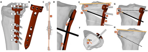
Figure 5. Qualitative evaluation of the preoperative planning solutions based on the ratings of three surgeons and two biomedical engineers. The individual ratings per case and reader are shown for the manual (A) and algorithm (B) solutions. The bar chart (C) represent the mean ratings for the manual and algorithm solutions for all 53 patient cases.

2.4.1.5. Implementation details

The MOO was implemented in Matlab (Matlab 2021a, The MathWorks Inc., Natick, MA, USA) using the genetic algorithm for multiobjective optimization from the Global Optimization toolbox. It applies a controlled elitist genetic algorithm (a variant of NSGA-II [44]). The algorithm parameters are summarized in Table 4. The first population in both stages is initialized using the default option in Matlab, which uses a quasirandom Sobol sequence to generate a well-dispersed population of chromosomes [57]. The default functions for mutations and crossover were used.

Table 4. Parameters of the multiobjective optimization algorithm.

Stage	1	2
Max # of generations	200	200
Parameters in chromosome	5	12
Number of objectives	2	3
Function tolerance	0.01	0.01
Pareto fraction	0.35	0.35

For the first stage, ${\mathrm{f}}_1$ and ${\mathrm{f}}_2$ were considered during the optimization: (12) $${\mathrm{X}}_{\mathrm{S}1}=\underset{\overrightarrow{x1}}{\mathit{arg min}}\left({\mathrm{w}}_1{\mathrm{f}}_1\right(\overrightarrow{x1}), {{\mathrm{w}}_2\mathrm{f}}_2(\overrightarrow{x1}\left)\right)$$(12) whereby ${\mathrm{X}}_{\mathrm{S}1}$ denotes the final pareto set of solutions after stage 1, $\overrightarrow{\mathrm{x}1}$ denotes the chromosome containing x1-5 and ${\mathrm{w}}_1= {\mathrm{w}}_2$ = 1.

After convergence, the solution with the lowest sum of ${\mathrm{f}}_1$ and ${\mathrm{f}}_2$ was chosen as the first stages’ final solution ${\overrightarrow{x}}_{s1}.$ (13) $${\overrightarrow{x}}_{s1}=\underset{{\overrightarrow{x}}_i\mathrm{ }\in \mathrm{ }{\mathrm{X}}_{\mathrm{S}1}}{\mathit{arg}\mathrm{ }\mathit{min}}\left({\mathrm{w}}_1{\mathrm{f}}_1\right({\overrightarrow{x}}_i)+\mathrm{ }{\mathrm{w}}_2{\mathrm{f}}_2({\overrightarrow{x}}_i\left)\right)$$(13)

For stage 2, all three fitness functions were considered based on the following weightening schema: (14) $${\mathrm{X}}_{\mathrm{S}2}=\underset{\overrightarrow{x2}}{\mathit{arg min}}\left({\mathrm{w}}_1{\mathrm{f}}_1\right(\overrightarrow{x2}), {{\mathrm{w}}_2\mathrm{f}}_2(\overrightarrow{x2}), {{\mathrm{w}}_3\mathrm{f}}_3(\overrightarrow{x2}\left)\right)$$(14) whereby ${\mathrm{X}}_{\mathrm{S}2}$ denotes the matrix holding the final pareto set of solutions after stage 2, $\overrightarrow{\mathrm{x}2}$ denotes the chromosome containing x1-12 and ${\mathrm{w}}_1= {\mathrm{w}}_2$ = 0.1 while ${\mathrm{w}}_3$ = 1.

To chose the final solution ${\overrightarrow{x}}_{s2}$ from the pareto set ${\mathrm{X}}_{\mathrm{S}2},$ we applied the following scheme: (15) $${\overrightarrow{x}}_{s2}=\underset{{\overrightarrow{x}}_i\mathrm{ }\in \mathrm{ }{\mathrm{X}}_{\mathrm{S}2}}{\mathit{arg}\mathrm{ }\mathit{min}}{f}_1\left({\overrightarrow{x}}_i\right)\mathrm{ }\left|\mathrm{ }{f}_3\right({\overrightarrow{x}}_i)\mathrm{ }\le \mathrm{ }p+m$$(15) whereby p = $\min \hspace{0.17em} f_3\left({\overrightarrow{x}}_j\right), {\overrightarrow{x}}_j \in \mathrm{ }{\mathrm{X}}_{\mathrm{S}2}$ and $m$ is an empirically determined margin set to 0.2.

To keep the optimization time as short as possible for simpler cases but still allow to find solutions for more complex cases, stage 2 was implemented as follows: The algorithm was run with a population size of 400. Whenever it was either not able to find a solution at all or the weighted sum of all fitness functions (see Equation (14)(14) $${\mathrm{X}}_{\mathrm{S}2}=\underset{\overrightarrow{x2}}{\mathit{arg min}}\left({\mathrm{w}}_1{\mathrm{f}}_1\right(\overrightarrow{x2}), {{\mathrm{w}}_2\mathrm{f}}_2(\overrightarrow{x2}), {{\mathrm{w}}_3\mathrm{f}}_3(\overrightarrow{x2}\left)\right)$$(14) ) was higher than 2, the population size was increased by 100 and the algorithm was rerun, up to a maximal population size of 1000.

2.5. Experiments/evaluation

2.5.1. Data

The pipeline was evaluated using a large database of retrospective cases of lower limb deformities. The study was approved by the local ethics committee and informed consent was obtained from all patients (Zurich Cantonal Ethics Commission, KEK 2018-02242).

All patients who underwent a tibial corrective osteotomy procedure in our institution between January 2015 and May 2020 and had a complete radiological dataset were included in the final evaluation of the pipeline. A full radiological dataset consisted of the following preoperative images:

• A biplanar standing long-leg radiograph (EOS imaging system, EOS, Paris, France)

• A CT scan (Philips Brilliance 64, Philips Healthcare, Best, The Netherlands, or Somatom Definition AS Siemens Healthcare, Erlangen, Germany) according to the MyOsteotomy CT protocol (Medacta SA, Switzerland). Hip, knee and ankle joints are scanned while the shaft regions were skipped to reduce radiation exposure. Slice thickness was 1 mm with a spacing of either 0.5 or 0.8 mm, in-plane resolution was either 0.2 or 0.4 mm. The slice size was 512 x 512 pixels, while the number of slices was different in every scan.

Patients with an incomplete radiological dataset were excluded, resulting in a total of 50 patients, of whom three patients were operated on both legs. Mean age at surgery was 44.3 ± 7.7 years, with 28 of the 53 legs were left legs, and a gender distribution of 39 males and 14 females. All of the patients suffered from varus deformities and therefore received a medial OWHTO.

2.5.2. Gold standard manual 3D planning

Biomedical engineers conducted manual preoperative planning in 3D for all 53 cases previous to the surgery, which was executed in our institution. The deformity assessment was performed as described in section Manual 3D deformity assessment. Based on the results, the surgeons determined the postoperative target values for MA and TS and the engineers manually combined all osteotomy parameters (e.g. location and direction of osteotomy axis, osteotomy plane, fixation plate, etc.). The planning was performed in our in-house planning software CASPA (CASPA 5.32, University Hospital Balgrist, Zurich, Switzerland).

2.5.3. Verification and validation

For our experiments, the target values ${\mathrm{\Phi }}_{MA}$ and ${\mathrm{\Phi }}_{TS}$ for the optimization were set to the same values for MA and TS which were chosen by the biomedical engineers in the manual preoperative planning of our patients. The final results of the pipeline were assessed both in quantitative accuracy (given the predefined target values for MA and TS) as well as qualitative feasibility. To this end, we asked three surgeons (two seniors (R1, R2), one attending (R3)) and two biomedical engineers (one senior (R4), one junior (R5)), to independently evaluate the automated as well as the previously performed manual preoperative planning solutions for each of the 53 cases. They were not directly involved in the development of the pipeline but were asked for feedback on the generated solutions at an intermediate stage. This feedback was further used to improve the algorithm parameter and constraints. After the algorithm was finalized, they graded both solutions in a blinded manner and categorized them into not acceptable, acceptable (could serve as the basis for preoperative planning), good (minor corrections required) and excellent (no corrections required). The evaluation was based on the positioning of the osteotomy axis as well as the cutting plane and the placement of the fixation plate including the screws. The readers were asked to give a reason for their grading whenever it was not excellent.

Adiditonal to the final planning solutions, we evaluated the performance of the individual components of the pipeline in the first two modules M1 and M2. The automatically segmented 3D models were assessed using the dice coefficient and the accuracy of the DL network for landmark localization was determined in terms of mean Euclidean distance between the predicted and the manually annotated (ground truth) landmarks. Moreover, the resulting deviation in the MA angle was calculated and the normal vector of the automatically fitted slope plane was projected to the sagittal plane and compared to the manually annotated, sagittally projected ground truth vector. The mean angular deviation was measured in degrees.

3. Results

A NVIDIA Quadro RTX 6000 with 24 GB RAM was used for training and testing the networks as well as running the MOO algorithm.

3.1. Module 1 - segmentation and landmark localization

The mean dice coefficients for the bone model segmentations were 0.98 ± 0.0, 0.98 ± 0.02, 0.95 ± 0.11 and 0.96 ± 0.05 for femur, tibia, patella and fibula.

The mean translational errors for hip, knee and ankle localization in 3D from the ten-fold cross validation were 1.3 ± 0.8 mm (range 0.2 − 5.9 mm), 1.8 ± 1.4 mm (range 0.2 − 11.6 mm) and 1.7 ± 0.9 mm (range 0.3 − 5.1 mm), respectively. The number of landmarks with an error below 2 mm were 90%, 71%, and 70%, respectively. The mean resulting deviation from the manually annotated MA was 0.1 ± 0.2°. The angular deviation in the sagittal plane between the ground truth and the automatically calculated slope normal vector $n_S$ was 1.5 ± 1.1°. Training a segmentation network for one fold took about 75, 270 and 75 min for hip, knee and ankle CTs. 3D Landmark localization networks were trained for about 40 min for stage 1 and 90 min for stage 2.

3.2. Module 2 - registration

The 2D–3D registration approach was previously published [19] and we therefore summarize the respective results here. The registration accuracy was evaluated using a sawbone model, to which we attached metal beads for the calculation of the ground truth translation between CT and EOS. The translation error between ground truth transformation and registration was 1.1, 0.3 and −0.1 mm and 0.0, 0.5 and −0.4 mm for femur and tibia in x, y and z direction, respectively. The resulting Euclidean distance was 1.1 mm and 0.6 mm for femur and tibia. The rotational errors were 0.0°, 0.1° and 1.2° for the femur and 0.0°, −0.2° and 1.1° for the tibia around x-, y- and z-axes. Clinical evaluation proved feasibility on real patient data. The mean difference for the MA was 2.1 ± 1.7°, 37.3% of the patients had differences of 2° or more between the weight-bearing and non-weight-bearing states.

3.3. Module 3 - multiobjective optimization

Five expert readers evaluated the algorithm’s preoperative solutions in a blinded manner. They used gradings from 0 to 3, corresponding to the categories not acceptable (0), acceptable (1), good (2) and excellent (3). The MOO algorithm was able to find solutions for all 53 cases. The mean absolute errors between the given target values for MA and TS and the achieved values in the algorithm solutions were 0.02° ± 0.05° and 0.02° ± 0.09°, respectively. Convergence of stage 1 took around one minute. Stage 2 terminated after roughly 80 min on average.

The mean score for the manual solutions was 2.3 ± 0.7, while the algorithm solutions were rated with 2.6 ± 0.6 on average. The 265 ratings for the manual solutions (5 readers and 53 cases) were distributed in 1.9% (5) not acceptable, 11.3% (30) acceptable, 44.5% (118) good and 42.3% (112) excellent, while the same distribution for the algorithm solutions was 0% (0) not acceptable, 5,3% (14) acceptable, 29.1% (77) good and 65.7% (174) excellent. The five surgeons and engineers rated the algorithm solution equally good or better than the manual solution in 89.4% (237) of all 265 comparisons. No differences were found between male vs. female patient cases, or between left vs. right legs. The results are displayed in Figure 5(B).

3.3.1. Parameter analysis

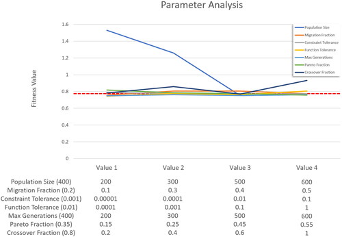
A sensitivity analysis was performed to determine how the genetic algorithm’s performance is affected by its settings. To achieve this, we reduced the algorithm’s runtime significantly by removing the computationally expensive penetration and distance checks of the fixation plate check points from the nonlinear constraints (g2 in the Constraints section). Even though the simplified version allows for small penetrations of the plate to the bone, it still produced very good solutions as the third fitness function penalizes both, severe penetrations and large gaps between plate and bone. When analyzing the results, it should be noted that the simplified constraints allow for more solutions and make it easier for the algorithm to find solutions (for example, with a smaller population size). This can result in slightly lower fitness values being generated compared to when the full version of the algorithm is applied.

Figure 6 shows the resulting mean fitness values after running the simplified algorithm for all 53 patient cases with varying parameters. For each parameter, four values were chosen, usually two below and two above the value used for the full version of the algorithm. Fort each parameter, the algorithm was run four times, with the value for the parameter being changed each time. All other parameters were set to their default value.

Figure 6. Parameter analysis. Resulting mean fitness value after varying several algorithm parameters in the simplified algorithm. The dashed line shows the final fitness value of 0.78 which was achieved by the full version of the algorithm with the default parameter settings (shown in brackets).

4. Discussion

The growing field of computer technologies in orthopedic surgery has also brought a change in surgical planning. Traditional 2D planning, based on simple line and angle calculations in 2D, has increasingly been replaced by 3D preoperative planning using CT-reconstructed bone models. However, the additional DoF also bring additional complexity, clear guidelines do not exist yet and computer-aided 3D planning is therefore laborious and highly dependent on the experience and skills of the human planner. Therefore, automating the preoperative planning seems reasonable and promises not only a reduction in effort and costs, but also objectification and standardization of the planning process. Its realization however is challenging; a wide range of clinical requirements and the extensive expertise of surgeons and engineers have to be translated into mathematical problems and adequate algorithms that can be performed by computation.

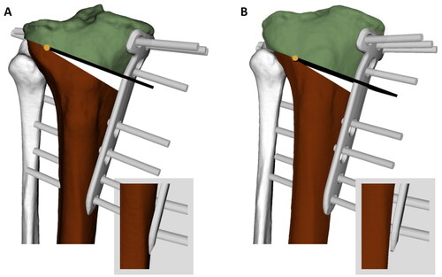
The evaluation obtained for our pipeline has shown that OWHTO planning can be successfully automated. The tedious processes of segmentation, annotation, coordinate system alignment, deformity measurement and weight-bearing transformation as well as the placement of osteotomy axis, cutting plane and fixation plate ran in a completely automated fashion. In addition, the target values for MA and TS were achieved very accurately. Our readers rated all automated planning solutions except one as good or excellent on average, and their overall mean rating was higher than the scores for the manual solutions. In seven cases, the mean rating for automated solutions was slightly lower than their corresponding manual solutions. The main point of criticism was the placement of the fixation plate, which was found to be too posterior and had small gaps between the plate and bone. Besides, the osteotomy axis was sometimes placed too distally as we chose a conservative strategy in selecting safety margins to avoid the risk of intraarticular fractures (see constraint g8). These problems can be addressed by further adjusting the algorithm constraints. Patient-specific fixation plates on the other hand are a promising approach to reduce gaps between the plate and the bone. Figure 7 shows both the manual and algorithm solution for the same case as an example for an improved solution generated by the algorithm.

Figure 7. Comparison between automated and manual solutions of one case. (A) Manual solution: The plate is placed too proximal and therefore, the screws are very close to the tibial plateau, which causes a high risk for fractures into the plateau. The screw S4 is located too close to the cut. Furthermore, the distal end of the plate penetrates the bone. (B) Algorithm solution: The osteotomy axis and cut as well as the plate is placed more distally, leaving enough security margin between screws and tibial plateau. Screw S4 has enough distance to the osteotomy cut and the distal end of the plate does not penetrate the bone.

The ratings have shown a relatively high degree of dissonance between the readers. Surgeons and engineers focus on different aspects (e.g. plate placement or osteotomy cut) based on their experience and background. In addition, they sometimes evaluate certain points with different degrees of importance, which leads to very different ratings. However, we could successfully adapt the algorithm parameters based on their feedback at an intermediate stage, such that the solutions of the algorithm corresponded to solutions on which clinical experts agree. They can therefore be used to generate baseline and ready-to-use preoperative solutions. This baseline can be further adapted to personal preferences or patient-specific requirements by adjusting constraints or changing the relative weighting of clinical objectives. Our approach does not only save time (it takes around 2 h of expert work per case to manually perform every task which is included in our pipeline), but successfully tackles the previously mentioned challenge of balancing automation and adaptability as well as the incorporation of clinical expertise. Using such a fully automated, adaptable framework, surgeons could calculate multiple solutions based on different user-defined criteria without spending additional time in front of the computer.

As part of the pipeline, we have trained DL networks to automatically segment the 3D bone models from CT scans as well as localize the required landmarks for deformity assessment. The segmentation accuracy was very similar to previous studies [58,59]. For landmark localization, our objective was to identify a single landmark in the CT scans of hip, knee, and ankle joints, respectively. As a consequence, we cannot benefit from learning the spatial configuration of multiple landmarks in the same image. Our error for the KJC and the AJC was higher than the mean error of the landmarks localized by Zhao et al. [43]. When investigating the cases with KJC errors higher than 4 mm, we found that all of them had either burr holes or metal implants from previous surgeries or severe anatomical abnormalities. The AJC on the other hand is not directly defined based on a shape feature but as the center of mass of all tibial and fibular articular surface points. Therefore, its localization with respect to e.g. the bone contours of the talus varies slightly and makes its localization more challenging.

Payer et al. [42] attributed their good performance to their data augmentation regime including elastic and intensity transformations, which could also be a viable approach to further improve the performance of our landmark localization module. Additionally, deep-learning based strategies such as inpainting and more diverse datasets could help to increase the network’s robustness toward metal parts or other abnormalities.

The registration module allows to bring the CT-reconstructed 3D models into a weight-bearing state. In previous studies, we have shown that approximately 40% of all patients have a difference of at least 2° and up to 6.2° between the frontal alignment in the loaded and unloaded states, and that there is an average difference of about 2° [10,19]. Such a difference is relevant for planning. The extent to which the loaded and unloaded values of frontal alignment are considered when calculating the correction angle is up to the responsible surgeon. This decision should be based on multiple clinical aspects, such as the range of motion, the state of the ligaments, the degree of degeneration as well as the patient’s activities.

Our pipeline was validated using 53 real patient datasets, which is to the best of our knowledge the largest series of patients in the literature with a CT scan and biplanar standing radiographs. The dataset contains cases with severely deformed bones or patients which were previously operated and therefore had burr holes or metal implants in their imaging data. This broad range of patient cases was challenging especially for the definition of the constraints during the MOO framework implementation, but at the same time ensures the pipeline’s generalizability.

Our protocol requires both a full CT scan of the entire leg and a biplanar standing radiograph, which, depending on the clinic, is not always part of the standard protocol. The acquisition of standing radiographs is part of the standard workflow everywhere, and highly specialized centers use the EOS system to significantly reduce the radiation exposure and acquire biplanar images in a 90° angle. The proposed registration approach could also be implemented for standard uniplanar full-leg standing radiography in order to align the 3D models to the standing position in the frontal plane. Compared to radiography, the acquisition of CT scans exposes the patient to more radiation and has to be considered carefully. Therefore, our CT protocol skips the shaft regions of femur and tibia. Technological developments, such as ultra low-dose CT or bone MRI, could be used in the future to further reduce the radiation dose.

Image-free approaches for navigation and intraoperative planning have been proposed [60] but were found to produce poor results in axial and sagittal planes [61]. The deformity is intraoperatively assessed based on pointer-acquired landmarks in the supine position and the subsequent planning does not consider the patient-specific anatomy or plate and screw positioning.

As a limitation, we want to address the possible dependency of our gold standard solutions on the experience of the involved planners, as we have used the solutions that were implemented in the respective surgeries at that time. As described in section Manual 3D deformity assessment, our manual annotations are performed in an in-house developed preoperative planning software which supports a standardized landmark annotation and reduces the differences between the readers. The agreement in landmark annotation between readers was assessed in a previous study [10], resulting in very good intraclass correlation coefficient for MA measurement [0.988 (95% CI: 0.981–0.992)]. Similarly, the segmentation is performed in a standardized, semi-automatic way which is widely used in literature and has been validated previously [62]. Finally, the final planning solutions were developed in multiple revision rounds between surgeons and engineers, ensuring the quality of the solutions. It was recently shown that significant variabilities exist only between planners with different levels of experience, but not between experienced planners [63].

Our MOO algorithm has shown to be very well capable of producing solutions for all patients, which were rated as good or excellent in all but one case. In this one case, the plate was still placed too close to the articular surface of the tibia. Moreover, for a few cases, it took very long to find a good solution (up to 7.5 h in one case). This is usually due to difficult anatomical conditions or the very strict constraints and low thresholds for rerunning stage 2 (fitness value lower than 2). In 90% of all cases the algorithm terminated within 2 h, which is however still too long for interactive adaptations by a user. One option would be to calculate a baseline solution and adapt it from there with a significantly reduced search space and therefore shorter optimization times.

So far, we have implemented our pipeline for a medial OWHTO, since all patients in our cohort had varus deformities. Future work could include the option for closing wedge as well as double osteotomies (femoral and tibial), which will bring new challenges such as defining a second osteotomy cut and additional constraints. Manual planning of double osteotomies is highly complex; it’s automation would therefore significantly increase the planning capabilities. The calculation of the mechanical medial proximal tibial angle (mMPTA) as well as the mechanical distal lateral femoral angle (mDLFA) could be easily implemented and considered when choosing the most appropriate surgical strategy.

Although we have showcased the capabilities of the method only on the plate model used in our institution, plates from other manufacturers can be easily integrated. Cadaver experiments could be used to compare planned and actual interventions for osteotomy and fixation plate placement. Lastly, it is conceivable that in the future, the CT scan will be replaced by a 3D reconstruction based on two (or more) 2D radiographs. While it has already been approached by using statistical shape models (SSM) [64], the use of patient specific intstruments (PSI) requires a higher accuracy than SSMs can provide in the case of highly pathological cases. Recently, Kasten et al. successfully used DL to reconstruct a knee joint from biplanar radiographs [50].

Currently, our modules are still implemented on different platforms and therefore it still requires manual work to transfer the results. However, each of the modules is completely automated and replaces a previously laborious manual process. The reported times are only computational and do not require any additional interaction with the user. The combination of all modules into one integrated solution, using the same software platform, could make the laborious part of the preoperative planning of OWHTO largely independent of human users.

Disclosure statement

No potential conflict of interest was reported by the author(s).

Data availability statement

The datasets analyzed during the current study are not publicly available due to individual privacy reasons but are available from the corresponding author upon reasonable request.

Additional information

Funding

This work was supported by the Swiss National Science Foundation under Grant No. 320030_182352/1.

References

- Paley D, Maar DC, Herzenberg JE. New concepts in high tibial osteotomy for medial compartment osteoarthritis. Orthop Clin North Am. 1994;25(3):483–498.
- Lee SS, Kim JH, Kim S, et al. Avoiding overcorrection to increase patient satisfaction after open wedge high tibial osteotomy. Am J Sports Med. 2022;50(9):2453–2461. 20:3635465221102144.
- Hernigou P, Medevielle D, Debeyre J, et al. Proximal tibial osteotomy for osteoarthritis with varus deformity. A ten to thirteen-year follow-up study. J Bone Joint Surg Am. 1987;69(3):332–354.
- Nha KW, Kim HJ, Ahn HS, et al. Change in posterior tibial slope After open-wedge and closed-wedge high tibial osteotomy: a meta-analysis. Am J Sports Med. 2016;44(11):3006–3013.
- Giffin JR, Vogrin TM, Zantop T, et al. Effects of increasing tibial slope on the biomechanics of the knee. Am J Sports Med. 2004;32(2):376–382.
- Voos JE, Suero EM, Citak M, et al. Effect of tibial slope on the stability of the anterior cruciate ligament-deficient knee. Knee Surg Sports Traumatol Arthrosc. 2012;20(8):1626–1631.
- Yamaguchi KT, Cheung EC, Markolf KL, et al. Effects of anterior closing wedge tibial osteotomy on anterior cruciate ligament force and knee kinematics. Am J Sports Med. 2018; Feb46(2):370–377.
- Hodel S, Zindel C, Jud L, et al. Influence of medial open wedge high tibial osteotomy on tibial tuberosity-trochlear groove distance. Knee Surg Sports Traumatol Arthrosc. 2023;31(4):1500–1506.
- Paley D. Principles of deformity correction. Berlin, Heidelberg: Springer; 2002.
- Jud L, Roth T, Furnstahl P, et al. The impact of limb loading and the measurement modality (2D versus 3D) on the measurement of the limb loading dependent lower extremity parameters. BMC Musculoskelet Disord. 2020;21(1):418.
- Fürnstahl P, Schweizer A, Graf M, et al. Surgical treatment of long-bone deformities: 3D preoperative planning and patient-specific instrumentation. In: Zheng G, Li S, editors. Computational radiology for orthopaedic intervensions. Vol. 23. Cham: Springer; 2016.
- Roth T, Rahm S, Jungwirth-Weinberger A, et al. Restoring range of motion in reduced acetabular version by increasing femoral antetorsion - What about joint load? Clin Biomech. 2021;87:105409.
- Munier M, Donnez M, Ollivier M, et al. Can three-dimensional patient-specific cutting guides be used to achieve optimal correction for high tibial osteotomy? Pilot study. Orthop Traumatol Surg Res. 2017;103(2):245–250.
- Ewurum CH, Guo Y, Pagnha S, et al. Surgical navigation in orthopedics: workflow and system review. Adv Exp Med Biol. 2018;1093:47–63.
- Chen AF, Kazarian GS, Jessop GW, et al. Robotic technology in orthopaedic surgery. J Bone Joint Surg Am. 2018;100(22):1984–1992.
- Joskowicz L, Hazan EJ. Computer aided orthopaedic surgery: incremental shift or paradigm change? Med Image Anal. 2016;33:84–90.
- Carrillo F, Vlachopoulos L, Schweizer A, et al. editors. A time saver: optimization approach for the fully automatic 3D planning of forearm osteotomies. Cham: Springer International Publishing; 2017.
- Vercauteren T, Unberath M, Padoy N, et al. CAI4CAI: the rise of contextual artificial intelligence in computer assisted interventions. Proc IEEE Inst Electr Electron Eng. 2020;108(1):198–214.
- Roth T, Carrillo F, Wieczorek M, et al. Three-dimensional preoperative planning in the weight-bearing state: validation and clinical evaluation. Insights Imaging. 2021;12(1):44.
- Eck M, Hoschek J, Weber U. Three-dimensional determination of an oblique osteotomy in the hip by mathematical optimization fulfilling some anatomical demands. J Biomech. 1990;23(10):1061–1067.
- Schkommodau E, Frenkel A, Belei P, et al. Computer-assisted optimization of correction osteotomies on lower extremities. Comput Aided Surg. 2005;10(5-6):345–350.
- Belei P, Schkommodau E, Frenkel A, et al. Computer-assisted single- or double-cut oblique osteotomies for the correction of lower limb deformities. Proc Inst Mech Eng H. 2007;221(7):787–800.
- Spellucci P. Numerische verfahren der nichtlinearen optimierung. Basel: Birkhäuser; 1993.
- Carrillo F, Roner S, von Atzigen M, et al. An automatic genetic algorithm framework for the optimization of three-dimensional surgical plans of forearm corrective osteotomies. Med Image Anal. 2020;60:101598.
- Caprara S, Fasser MR, Spirig JM, et al. Bone density optimized pedicle screw instrumentation improves screw pull-out force in lumbar vertebrae. Comput Methods Biomech Biomed Engin. 2021;9:1–11.
- Hill D, Williamson T, Lai CY, et al. Automated resection planning for bone tumor surgery. Comput Biol Med. 2021;137:104777.
- Lambrechts A, Wirix-Speetjens R, Maes F, et al. Artificial intelligence based patient-specific preoperative planning algorithm for total knee arthroplasty. Front Robot AI. 2022;9:840282.
- Yue Y, Gao Q, Zhao M, et al. Prediction of knee prosthesis using patient gender and BMI With non-marked X-Ray by deep learning. Front Surg. 2022;9:798761.
- Tschannen M, Vlachopoulos L, Gerber C, et al. Regression forest-based automatic estimation of the articular margin plane for shoulder prosthesis planning. Med Image Anal. 2016;31:88–97.
- Kulyk P, Vlachopoulos L, Fürnstahl P, et al. editors. Fully automatic planning of total shoulder arthroplasty Without segmentation: a deep learning based approach. Cham: Springer International Publishing; 2019.
- Ackermann J, Wieland M, Hoch A, et al. editors. A new approach to orthopedic surgery planning using deep reinforcement learning and simulation. Cham: Springer International Publishing; 2021.
- Esfandiari H, Anglin C, Guy P, et al. A comparative analysis of intensity-based 2D-3D registration for intraoperative use in pedicle screw insertion surgeries. Int J Comput Assist Radiol Surg. 2019;14(10):1725–1739.
- Risholm P, Golby AJ, Wells W. 3rd. Multimodal image registration for preoperative planning and image-guided neurosurgical procedures. Neurosurg Clin N Am. 2011;22(2):197–206, viii.
- Postolka B, List R, Thelen B, et al. Evaluation of an intensity-based algorithm for 2D/3D registration of natural knee videofluoroscopy data. Med Eng Phys. 2020;77:107–113.
- Yamazaki T, Watanabe T, Nakajima Y, et al. Improvement of depth position in 2-D/3-D registration of knee implants using single-plane fluoroscopy. IEEE Trans Med Imaging. 2004;23(5):602–612.
- Matsushita T, Watanabe S, Araki D, et al. Differences in preoperative planning for high-tibial osteotomy between the standing and supine positions. Knee Surg Relat Res. 2021;33(1):8.
- Schoenmakers DAL, Feczko PZ, Boonen B, et al. Measurement of lower limb alignment: there are within-person differences between weight-bearing and non-weight-bearing measurement modalities. Knee Surg Sports Traumatol Arthrosc. 2017;25(11):3569–3575.
- Wieser K, Furnstahl P, Carrillo F, et al. Assessment of the isometry of the anterolateral ligament in a 3-dimensional weight-bearing computed tomography simulation. Arthroscopy. 2017;33(5):1016–1023.
- Kobayashi K, Sakamoto M, Tanabe Y, et al. Automated image registration for assessing three-dimensional alignment of entire lower extremity and implant position using bi-plane radiography. J Biomech. 2009; 42(16):2818–2822.
- Noothout JMH, de Vos BD, Wolterink JM, et al. Deep learning-based regression and classification for automatic landmark localization in medical images. IEEE Trans Med Imaging. 2020;39(12):4011–4022.
- Payer C ,Štern D, Bischof H, et al. editors. Regressing heatmaps for multiple landmark localization using CNNs. Cham: Springer International Publishing; 2016.
- Payer C, Stern D, Bischof H, et al. Integrating spatial configuration into heatmap regression based CNNs for landmark localization. Med Image Anal. 2019;54:207–219.
- Zhao QJ, Zhu JH, Zhu JJ, et al. Bone anatomical landmark localization with cascaded spatial configuration network. Meas Sci Technol. 2022;33(6):065401.
- Kalyanmoy D. Multi-Objective optimization using evolutionary algorithms. Chichester, England: John Wiley & Sons; 2001.
- Lorensen WE, Cline HE, editors. Marching cubes: a high resolution 3D surface construction algorithm. ACM siggraph computer graphics. ACM; 1987.
- Roscoe L. Stereolithography interface specification. America-3D Systems Inc.; 1988.
- Schneider P, Eberly DH. Geometric tools for computer graphics. Elsevier; 2002.
- Eberly D. Least squares fitting of data. Chapel Hill (NC): Magic Software; 2000. p. 1–10.
- Ronneberger O, Fischer P, Brox T, editors. U-Net: convolutional networks for biomedical image segmentation. Cham: Springer International Publishing; 2015.
- Kasten Y, Doktofsky D, Kovler I, editors. End-to-end convolutional neural network for 3D reconstruction of knee bones from bi-planar X-ray images. International Workshop on Machine Learning for Medical Image Reconstruction. Lima: Springer; 2020.
- Abadi M, Barham P, Chen J, et al. editors. {TensorFlow}: a system for {Large-Scale} machine learning. In: 12th USENIX symposium on operating systems design and implementation (OSDI 16). 2016.
- Torr PHS, Zisserman A. MLESAC: a new robust estimator with application to estimating image geometry. Comput Vision Image Understanding. 2000;78(1):138–156.
- Markelj P, Tomazevic D, Likar B, et al. A review of 3D/2D registration methods for image-guided interventions. Med Image Anal. 2012;16(3):642–661.
- LaRose D. Iterative X-Ray/CT registration using accelerated volume rendering. Pittsburgh (PA): Carnegie Mellon University; 2001.
- Powell MJD. The BOBYQA algorithm for bound constrained optimization without derivatives. 2009.
- Johnson SG. The NLopt nonlinear-optimization package. http://github.com/stevengj/nlopt
- Sobol IM. On the distribution of points in a cube and the approximate evaluation of integrals. USSR Computational Mathemat Mathemat Phys. 1967;7(4):86–112.
- Marzorati D, Sarti M, Mainardi L, et al. Deep 3D convolutional networks to segment bones affected by severe osteoarthritis in CT scans for PSI-based knee surgical planning. IEEE Access. 2020;8:196394–196407.
- Maintier L ,Maguet E, Clavé A, et al. editors. Tibial and femoral bones segmentation on CT-scans: a deep learning approach. In: Proceedings of the 20th annual meeting of the interna. 2022.
- Lorenz S, Morgenstern M, Imhoff AB. Development of an image-free navigation tool for high tibial osteotomy. Operat Techniq Orthopaed. 2007;17(1):58–65.
- Pearle AD, Goleski P, Musahl V, et al. Reliability of image-free navigation to monitor lower-limb alignment. J Bone Joint Surg Am. 2009;91:90–94.
- Cook DJ, Gladowski DA, Acuff HN, et al. Variability of manual lumbar spine segmentation. Int J Spine Surg. 2012;6:167–173.
- Zindel C, Furnstahl P, Hoch A, et al. Inter-rater variability of three-dimensional fracture reduction planning according to the educational background. J Orthop Surg Res. 2021;16(1):159.
- Zheng G, Hommel H, Akcoltekin A, et al. A novel technology for 3D knee prosthesis planning and treatment evaluation using 2D X-ray radiographs: a clinical evaluation. Int J Comput Assist Radiol Surg. 2018;13(8):1151–1158.