Throughput control and revenue optimization of a poultry product batcher

Abstract

This article studies the optimal control of batching equipment in the poultry processing industry. The problem is to determine a control policy that maximizes the long-term average revenue while achieving a target throughput. This problem is formulated as a Markov Decision Process (MDP). The developed MDP model captures the unique characteristics of poultry processing operations, such as, the trade-off between giveaway and throughput. Structural properties of the optimal policy are derived for small-sized problems where batching equipment utilizes a single bin. Since the MDP model is numerically intractable for industry-sized problems, we propose a heuristic index policy with a Dynamic Rejection Threshold (DRT). The DRT heuristic is constructed based on the salient characteristics of the problem setting and is easy to implement in practice. Numerical experiments demonstrate that DRT performs well. We present an industry case study where DRT is benchmarked against current practice, which shows that the expected revenue can be potentially increased by over 2% (yielding an additional revenue between 750,000 and 2,270,000 Euros per year) through the use of DRT.

Keywords:

• Bin-covering problem
• Markov decision processes
• index policies
• case study

1. Introduction

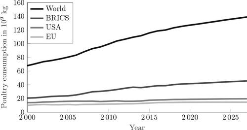
Global poultry meat consumption is projected to grow in the foreseeable future (OECD, 2017), as shown in Figure 1. Especially emerging markets such as Brazil, Russia, India, China, and South-Africa (BRICS) contribute to this projected growth. In more developed markets such as Europe or the United States, the demand for poultry products is saturated, which has led to increased pressure on the profit margins. However, retailers are large and powerful, and are able to put much of this pressure on their suppliers instead (Manning and Baines, 2004). Consequently, poultry processing plants experience increasing financial challenges, forcing them to explore new avenues for cost reduction in order to remain competitive. In this article, we consider the perspective of a poultry processing plant that faces demand from retailers, and aims to maximize their revenue through novel production control policies.

Figure 1. Past and forecasted poultry consumption per year for selected regions (OECD, 2017)

Farmers breed broilers before delivering them to poultry processing plants. At these plants, broilers are processed into a variety of final products (e.g., fillets, legs or wings). A processing plant using high-end equipment is typically capable of processing 15,000 broilers per hour for 16 hours per day. Each broiler can be sold as whole or processed into different parts, and packaged according to customer demand. The majority of demand comes from retailers, who impose a strict daily target throughput on poultry processing plants, i.e., they require a minimum amount of products produced per day. In addition, retailers require that each delivered (retail) batch contains a pre-specified target weight and pay a fixed price per batch of products. Additional weight over this target weight is not paid for, and is called giveaway. These retail batches are the packaged products one can purchase at supermarkets. The remaining demand comes from customers such as restaurant chains, who impose no target throughput. Such customers order large batches of products (bulk batch) rather than retail batches. Processing plants are paid for all weight in a bulk batch (i.e., no giveaway), although the price per unit weight of a bulk batch is lower compared with a retail batch.

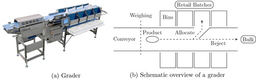
Batchers are machines used to produce retail batches. Figure 2(a) shows a grader, which is a batcher typically used in poultry processing plants. A schematic overview of this machine is shown in Figure 2(b). Each item arriving on the conveyor is weighed and placed in one of the available bins or rejected. A grader producing retail batches is allowed to reject items and send them to a downstream process that produces bulk batches. For practitioners, this leads to a critical trade-off between giveaway and throughput: by rejecting items, the giveaway can be reduced. However, rejecting items lowers the throughput, and may lead to a failure to comply with the target throughput. Therefore, we consider the following problem setting. A grader produces retail batches with a given target weight and target throughput. Each completed retail batch has a fixed value, and all rejected weight is processed as bulk batches, which have a lower value per gram. The goal is to simultaneously achieve the target throughput and maximize the overall revenue, by either allocating items to a bin in the grader, or rejecting them.

Figure 2. The batcher considered in this article.

The problem is relevant in practice, as the profit margins of processing plants are decreasing and giveaway reduction is an important avenue for cost reduction. For example, in a high-end processing plant, each percentage of giveaway reduction producing fillet batches is worth over a million Euro per year in revenue. Grader algorithms used in practice are able to control the fraction of items allocated to retail batches, but cannot control the throughput directly. It is challenging to achieve the target throughput, as throughput and giveaway are conflicting objectives, and the impact of the giveaway–throughput trade-off on the total expected revenue is not fully understood.

To address these challenges, we formulate a Markov Decision Process (MDP) model capturing the trade-off between giveaway and throughput. For a special case of the problem with a single bin and no throughput constraint, we show that optimal policies have a threshold-type structure on a subset of the state space. Due to the curse of dimensionality, the MDP model cannot be solved for industry-sized problems. In order to remedy this problem, a heuristic algorithm is developed, that is capable of achieving a given target throughput while minimizing the giveaway.

The heuristic introduced in this article is shown to be competitive with the MDP formulation for small-sized problems. The developed algorithm significantly outperforms the best-known heuristic, increasing revenue by up to 5% for the same target throughput. Testing this algorithm on a practically-relevant benchmark (provided by our industry partner) shows an increased revenue in all studied settings. In particular, our numerical analysis estimates that the revenue can potentially be increased between 750,000 and 2,270,000 Euros per year. Lastly, the revenue is studied for different target weights, throughput requirements, and relative values of bulk batches compared with retail batches. In numerical experiments, we anticipate revenue improvements up to 15% between different production settings, illustrating the high sensitivity of revenue to the production setting.

This article is organized as follows. In Section 2, literature relevant to this problem and the proposed algorithm are discussed. Next, Section 3 introduces the model describing the grader, item weights, and performance measures. Section 4 discusses heuristic grader policies, and the proposed extension to setting a target throughput. Simulation experiments are presented in Section 5, and our conclusions and recommendations for future work are summarized in Section 6.

2. Literature

The grader considered in this article has the property that products arrive one-by-one, products must be allocated or rejected immediately, and the grader can add products to batches in one of its bins. The problem of minimizing giveaway using such a batcher is known as an online K-bounded bin-covering problem with rejection. Online refers to the type of arrival process, K refers to the number of bins, and the bin-covering problem refers to the challenge of minimizing the long-term average overfill (giveaway) per bin.

Packing problems such as the bin-covering problem have been widely studied. Frequently, stylized off-line or unbounded problems are considered, which permit sorting of items and have an unlimited number of available bins. However, these assumptions might not be realistic for most production settings, as equipment and items have physical limitations. In this context, heuristics are typically necessary to deal with practically-sized problems. Csirik et al. (2001) introduce and analyze the Sum-of-Squares (SS) algorithm for bin covering that is online and bounded. Ásgeirsson (2014) introduces a prospect function to forecast the eventual giveaway of a bin and uses this function to develop algorithms for the online and bounded case. Similar to the prospect function, Peeters et al. (2017) introduce an index policy to predict giveaway and control multiple graders in parallel. Some research considers bin-covering problems with the option to reject items. Most algorithms developed in this context require a partitioning of item weights or an unbounded setting (Dósa and He, 2006; Correa and Epstein, 2008). Lastly, Peeters et al. (2019) introduce a heuristic based on an index function to control the throughput in an online and bounded setting. To the best of our knowledge, only Peeters et al. (2019) consider a problem setting similar to ours. However, Peeters et al. (2019) focus soley on developing a heuristic solution, and conduct a simulation study to assess its performance. In contrast, we build a stochastic optimization model for an online bin-covering problem with rejection, and exploit the structural properties of optimal policies. In addition, we enhance the heuristic proposed by Peeters et al. (2019) and study its performance both analytically and numerically.

Some studies employ exact methods such as Markov chains to solve packing problems. For instance, Asgeirsson and Stein (2006) and Asgeirsson and Stein (2009) utilize Markov chains to predict giveaway in different system states, and use the information to allocate products in their Min-Bin-State-Cost algorithm. Both consider an online and bounded setting. Coffman Jr et al. (1993) model the Best Fit algorithm as an infinite multi-dimensional Markov chain to analyze its performance. While online, Best Fit can only be used in an unbounded setting. Finally, Ásgeirsson (2014) introduces an MDP formulation of the online and bounded problem, and develops new heuristics based on the resulting optimal policies. In the current article, we continue the line of research of Asgeirsson and Stein (2006, 2009); Ásgeirsson (2014); Peeters et al. (2017); Peeters et al. (2019). They each study policies that utilize giveaway prediction in the form of index-type policies.

We summarize our contributions as follows:

1. We study a practically-relevant problem of optimizing batching and rejection decisions, and develop an MDP formulation (and a corresponding Linear Program formulation) for an online K-bounded bin-covering problem with rejection. Our model captures the salient features of poultry processing operations, such as, the trade-off between giveaway and throughput.

2. We analyze the structural properties of optimal policies, and show that optimal policies have a switching-curve structure under certain special cases (i.e., there exists a certain threshold value on item weight and bin weight, such that, it is optimal to only reject items when the system’s state exceeds these thresholds). However, we show that this switching-curve structure exists only for a subset of the state space (so called closing-states) under a special case of the problem with a single bin and no throughput requirement.¹

3. To solve industry-size problems, we develop a heuristic based on index policies. Our proposed heuristic adopts dynamic rejection thresholds to manage the giveaway–throughput trade-off. In addition, we prove that the proposed heuristic achieves the target throughput.

4. We present an industry case study to illustrate the use of the optimization approach and quantify its potential impact on practice. In addition, numerical experiments show that our proposed heuristic outperforms other best-known heuristics (e.g., Peeters et al. (2019), and current practice).

In summary, our models formalize our understanding on the online bin-covering problem in the poultry processing industry, and our results inform practitioners on the potential impact of the giveaway–throughput trade-off on the long-term average revenue.

3. Model

This section describes the problem of controlling a grader, and models the batching process. Section 3.1 provides a formal description of the grader, which is used in Section 3.2 to introduce the MDP model and corresponding Linear Program (LP) formulation. Structural results for the special case of a single bin with no throughput constraint are presented in Section 3.3. A summary of notation used throughout the paper is provided in online Appendix A.

3.1. Grader model

In practice, the grader is typically dedicated to a certain product type (e.g., fillets). In this setting, the grader is tasked with allocating items (e.g., fillets) to bins, or letting them pass to a bulk batching station as follows. Items arrive on a conveyor belt at the grader and are weighed to the nearest integer gram. The set of observed weights is $\mathcal{W}=\{w_{\text{min}},w_{\text{min}}+1,\dots ,w_{\text{max}}\}$ and p(w) is the probability that a product weighs w grams. The grader can place an arriving item in one of its K available bins or reject it. Bins are labeled 1 through K, and the set of available bins is $\mathcal{K}=\{1,2,\dots ,K\}.$ When bins are filled to their target weight B or more, they are emptied instantaneously (i.e., the target weight for each bin is B, and hence, giveaway is obtained when the weight of a bin exceeds the target weight B). The weight in bin $k\in \mathcal{K}$ is indicated as $v_k\in \mathcal{V}=\{0,1,\dots ,B-1\}.$ The interested reader can find a more detailed description of the production process in Peeters et al. (2017).

Let μ denote the average item weight and T the average inter-arrival time of products. So $\frac{\mu }{T}$ is the average weight arriving per time unit. Suppose that the due date of an order of Q batches with target weight B is D time units from now. Then the long-term target throughput of batched weight per time unit is $\frac{Q·B}{D},$ which should be less than $\frac{\mu }{T}.$ This translates to a target of batching a fraction $q=\frac{Q·B·T}{D·\mu }$ of the arriving weight per time unit. Hence, the goal is to allocate or reject items such that the revenue is maximized, under the condition that in the long term (at least) a fraction q of the arriving weight is batched. In Section 3.2, we present an MDP formulation of this problem.

3.2. MDP model

To define the MDP model, we need to specify states, actions, rewards and transitions. Decision epochs correspond with the arrivals of items. State $s=(v_1,\dots ,v_K,w)\in \mathcal{S}={\mathcal{V}}^K\times \mathcal{W}$ records the weights in all bins just before arrival of an item as well as the weight of the arriving item. Action $a\in \left\{0\right\}\cup \mathcal{K}$ denotes rejection of the arriving item if a = 0 and allocation of the item to bin a if $a\in \mathcal{K}.$ The normalized value of retail batches is 1 per gram and the normalized value of rejected weight is r_r per gram, where $0<r_r<1.$ The revenue for giveaway is zero, so the value of a batch of size $\ge B$ is equal to B. The revenue for batched weight is incurred when the batch is completed. The reward of action a in state $s=(v_1,\dots ,v_K,w)$ is denoted by $r(v_1,\dots ,v_K,w|a)$ and given by $$r(v_1,\dots ,v_K,w|a)\mathrm{}=\{\begin{array}{cc}0,\hspace{1em}\hfill & \text{if}\mathrm{}{v}_a+w<B,\mathrm{}\text{and}\mathrm{}a\in \mathcal{K},\hfill \\ B,\hspace{1em}\hfill & \text{if}\mathrm{}{v}_a+w\ge B,\mathrm{}\text{and}\mathrm{}a\in \mathcal{K},\hfill \\ r_r·w,\hspace{1em}\hfill & \text{if}\mathrm{}a=0.\hfill \end{array}$$

The probability of making a transition from state $s=(v_1,\dots ,v_K,w)$ to $s\prime =(v_1^{\prime },\dots ,v_K^{\prime },w\prime )$ when taking action a is denoted by $t(s\prime |s,a).$ This transition probability is given by (1) $$t(s\prime |s,a)=\{\begin{array}{c}p(w\prime ),\hspace{1em}\text{where}\mathrm{}s\prime =(v_1,\dots ,e(v_a+w),\dots ,v_K,w\prime )\mathrm{}\text{if}\mathrm{}a\in \mathcal{K},\hfill \\ p(w\prime ),\hspace{1em}\text{where}\mathrm{}s\prime =(v_1,\dots ,v_K,w\prime )\hspace{1em}\mathrm{}\text{if}\mathrm{}a=0,\hfill \end{array}$$(1) where the function e(x) is defined as $$e(x)\mathrm{}=\{\begin{array}{cc}x,\hfill & x<B,\hfill \\ 0,\hfill & x\ge B.\hfill \end{array}$$

The objective is to maximize the long-term average reward per item, provided the throughput target is met. To do so, we employ a LP formulation of the MDP (Derman, 1970). Let x_sa denote the long-term average fraction of times action $a\in \mathcal{A}$ is taken in state $s\in \mathcal{S}.$ To formulate the throughput constraint we note that the average weight per item allocated to the grader is (2) $$\sum _{s\in \mathcal{S}}\sum _{a\in \mathcal{K}}{x}_{sa}·w.$$(2)

The allocated weight can be divided into throughput weight and giveaway. Throughput weight is defined as the weight that is added to a batch below the target weight, and giveaway is the weight that is added more than the target weight of a batch. The long-term average giveaway per item is (3) $$\sum _{s\in \mathcal{S}}\sum _{a\in \mathcal{K}}{x}_{sa}·g(v_a+w),$$(3) where the giveaway function g(x) of a bin with weight $x\in \mathcal{W}$ is specified as (4) $$g(x)\mathrm{}=\{\begin{array}{cc}0,\hfill & x\le B,\hfill \\ x-B,\hfill & x>B.\hfill \end{array}$$(4)

Subtracting giveaway (3) from the allocated weight (2) yields the long-term average throughput weight per item. The throughput constraint states that this should be greater than or equal to a fraction q of the average item weight μ, in other words $$\sum _{s\in \mathcal{S}}\sum _{a\in \mathcal{K}}{x}_{sa}(w-g(v_a+w))\ge q·\mu$$

The LP formulation of the MDP now reads as follows: (5a) $${\underset{x}{\text{max}}}_{}\sum _{s\in \mathcal{S}}\sum _{a\in \mathcal{A}}r(s|a)x_{sa}$$(5a) (5b) $$\mathrm{s}.\mathrm{t}.\sum _{a\in \mathcal{A}}{x}_{s\prime a}-\sum _{s\in \mathcal{S}}\sum _{a\in \mathcal{A}}t(s\prime |s,a)x_{sa}=0,\hspace{1em}\mathrm{}\text{for}\mathrm{}\text{all}\mathrm{}s\prime \in \mathcal{S}$$(5b) (5c) $$\sum _{s\in \mathcal{S}}\sum _{a\in \mathcal{A}}{x}_{sa}=1$$(5c) (5d) $$\sum _{s\in \mathcal{S}}\sum _{a\in \mathcal{K}}{x}_{sa}(w-g(v_a+w))\ge q·\mu$$(5d) (5e) $$x_{sa}\ge 0,\hspace{1em}\mathrm{}\text{for}\mathrm{}\text{all}\mathrm{}s\in \mathcal{S}\mathrm{}\text{and}\mathrm{}a\in \mathcal{A}.$$(5e)

The objective of maximizing the long-term average reward per item is expressed by (5a). Equations (5b)(5b) $$\mathrm{s}.\mathrm{t}.\sum _{a\in \mathcal{A}}{x}_{s\prime a}-\sum _{s\in \mathcal{S}}\sum _{a\in \mathcal{A}}t(s\prime |s,a)x_{sa}=0,\hspace{1em}\mathrm{}\text{for}\mathrm{}\text{all}\mathrm{}s\prime \in \mathcal{S}$$(5b) are the balance equations. Equations (5c)(5c) $$\sum _{s\in \mathcal{S}}\sum _{a\in \mathcal{A}}{x}_{sa}=1$$(5c) and (5d)(5d) $$\sum _{s\in \mathcal{S}}\sum _{a\in \mathcal{K}}{x}_{sa}(w-g(v_a+w))\ge q·\mu$$(5d) are the normalization equation and the throughput constraint, respectively.

The above LP formulation may have no feasible solutions, i.e., the target of batching a fraction q of the arriving weight per unit may not be achievable. The LP problem below determines the maximal achievable target throughput $q^{*}:$ (6a) $${\underset{x}{\text{max}}}_{}\frac{1}{\mu }\sum _{s\in \mathcal{S}}\sum _{a\in \mathcal{K}}{x}_{sa}(w-g(v_a+w))$$(6a) (6b) $$\mathrm{s}.\mathrm{t}.\sum _{a\in \mathcal{A}}{x}_{s\prime a}-\sum _{s\in \mathcal{S}}\sum _{a\in \mathcal{A}}t(s\prime |s,a)x_{sa}=0,\hspace{1em}\mathrm{}\text{for}\mathrm{}\text{all}\mathrm{}s\prime \in \mathcal{S}$$(6b) (6c) $$\sum _{s\in \mathcal{S}}\sum _{a\in \mathcal{A}}{x}_{sa}=1$$(6c) (6d) $$x_{sa}\ge 0,\hspace{1em}\mathrm{}\text{for}\mathrm{}\text{all}\mathrm{}s\in \mathcal{S}\mathrm{}\text{and}\mathrm{}a\in \mathcal{A}.$$(6d)

The following theorem presents a necessary and sufficient condition for feasibility of the MDP.

Theorem 1.

LP problem (5a)-(5e) has a feasible solution if and only if $q\le q^{*}.$

Proof.

LP problem (6a)-(6d) is feasible, since the balance equations (6b)(6b) $$\mathrm{s}.\mathrm{t}.\sum _{a\in \mathcal{A}}{x}_{s\prime a}-\sum _{s\in \mathcal{S}}\sum _{a\in \mathcal{A}}t(s\prime |s,a)x_{sa}=0,\hspace{1em}\mathrm{}\text{for}\mathrm{}\text{all}\mathrm{}s\prime \in \mathcal{S}$$(6b) are feasible. Let $x_{sa}^{*}$ denote the solution with maximal target throughput $q^{*}.$ Then $x_{sa}^{*}$ is a feasible solution of (5b)-(5e) if $q\le q^{*}.$ On the other hand, if $q>q^{*},$ there can be no feasible solution of (5b)-(5e), since this solution would yield a target throughput exceeding $q^{*}$ which the maximal throughput. □

3.3. Structural results

To study the structural properties of optimal policies, we now consider a special case of the problem with a single bin (K = 1) and no throughput constraint. We focus on this special case because the theoretical analysis (Section 3.3) and numerical experiments (Section 5.3) indicate that optimal policies do not necessarily exhibit a structural behavior (even for the special case with a single bin). All proofs are available in online Appendix B.

To exclude that it is optimal to reject every arriving item, we assume in this section that (7) $$g_a>r_r\mu ,$$(7) where g_a is the average reward of the always-accept policy and $r_r\mu$ is the average reward of the always-reject policy. Let $a^{*}(v,w)$ denote an optimal action in state (v, w). Next, we derive structural properties of optimal actions in states (v, w) for which $v+w\ge B.$ Hereafter, these states will be referred to as closing-states.

Theorem 2.

For states (v, w) with $v+w\ge B$ there exist $w^{*}(v)$ such that $a^{*}(v,w)=1$ for $w<w^{*}(v)$, and $a^{*}(v,w)=0$ for $w\ge w^{*}(v).$

For a given bin level v, Theorem 2 characterizes the structural properties of optimal policies for closing-states. In particular, Theorem 2 indicates that, for given bin level v, there exists a threshold from which it is optimal to only reject items. This makes sense: once it is profitable to reject an item, this is also profitable for heavier items, as they result in the same immediate reward B but lead to higher giveaway. The next theorem is symmetrical to Theorem 2, stating that, for given item weight w (instead of bin level v), there exists a threshold from which it is optimal to only reject items.

Theorem 3.

For states (v, w) with $v+w\ge B$ there exist $v^{*}(w)$ such that $a^{*}(v,w)=1$ for $v<v^{*}(w)$, and $a^{*}(v,w)=0$ for $v\ge v^{*}(w).$

For closing-states (v, w) with $v+w\ge B,$ Theorems 2 and 3 indicate that rejection thresholds exist in both w and v. From a practical perspective, this result means that optimal policies have a switching-curve structure for closing-states. A visual representation of optimal policies are provided in Figure 7 for a problem setting with a single bin and no throughput constraint. As illustrated in Figure 7, optimal policies have a switching-curve structure for closing-states, although it is hard to derive structural properties on other parts of the state space.

In realistic settings, the state space of the MDP model will be “too big” for numerical calculations, i.e., the size of the state space is $B^k(w_{\text{max}}-w_{\text{min}}+1)$ and the size of the action space is k + 1. Observe that the space space grows exponentially in the number of bins k. For a standard industry-size problem with K = 8 bins (as presented in Section 5), the state space can easily reach a magnitude of 10²² states. Consequently, we turn to efficient approximate methods for online bin-covering problems. In Section 4, we present heuristic methods for controlling the grader with rejection.

4. Heuristic policies with rejection

Heuristic policies have been successfully used in bin-covering problems in a practical setting (Ásgeirsson, 2014; Peeters et al., 2017, Peeters et al., 2019). In this section, we formally describe policies that are typically used and motivate their use in our specific setting. Then, these policies are extended to allow for rejection of items.

First, we introduce some notation. For any allocation policy, the grader evolves as a Markov chain on state space $\mathcal{S}.$ In the following we assume this Markov chain is irreducible. After N items have been processed, the total throughput weight is denoted as the random variable $w_N^b,$ the total giveaway as $w_N^g$ and the total rejected weight as $w_N^r.$ When item N + 1 arrives with weight $w\in \mathcal{W}$ and finds weights $v_1,\dots ,v_K$ in the K bins (so the Markov chain is in state $s=(v_1,\dots ,v_K,w)$), these quantities are adapted depending on whether item N + 1 is accepted ($a\in \mathcal{K}$) or rejected (a = 0). Consistent with Peeters et al. (2019), this update procedure is modeled in (8): (8) $$\begin{array}{c}{w}_{N+1}^b=\{\begin{array}{cc}{w}_N^b+(w-g(v_a+w)),\hfill & \mathrm{}\text{if}\mathrm{}a\in \mathcal{K},\hfill \\ w_N^b,\hfill & \mathrm{}\text{if}\mathrm{}a=0,\hfill \end{array}\hfill \\ w_{N+1}^g\hfill & =\{\begin{array}{cc}{w}_N^g+g(v_a+w),\hfill & \mathrm{}\text{if}\mathrm{}a\in \mathcal{K},\hfill \\ w_N^g,\hfill & \mathrm{}\text{if}\mathrm{}a=0,\hfill \end{array}\hfill \\ w_{N+1}^r\hfill & =\{\begin{array}{cc}{w}_N^r,\hfill & \mathrm{}\text{if}\mathrm{}a\in \mathcal{K},\hfill \\ w_N^r+w,\hfill & \mathrm{}\text{if}\mathrm{}a=0.\hfill \end{array}\hfill \end{array}$$(8)

Let w_N denote the total weight of the first N items. Then we have: (9) $$w_N=w_N^b+w_N^g+w_N^r.$$(9)

By defining the fraction of throughput weight ${\overline{w}}_N^b=w_N^b/w_N,$ giveaway ${\overline{w}}_N^g=w_N^g/w_N,$ and rejected weight ${\overline{w}}_N^r=w_N^r/w_N,$ we obtain from (9) that: (10) $$1={\overline{w}}_N^b+{\overline{w}}_N^g+{\overline{w}}_N^r.$$(10)

Since the Markov chain is finite and irreducible, the time averages $w_N^b/N,w_N^g/N$ and $w_N^r/N$ converge as $N\to \infty$ with probability 1. Hence, also the long-term fraction of throughput weight ${\overline{w}}^b=\underset{N\to \infty }{\lim }{w}_N^b/w_N,$ giveaway ${\overline{w}}^g=\underset{N\to \infty }{\lim }{w}_N^g/w_N,$ and rejected weight ${\overline{w}}^r=\underset{N\to \infty }{\lim }{w}_N^r/w_N$ exist and, by (10), satisfy (11) $$1={\overline{w}}^b+{\overline{w}}^g+{\overline{w}}^r.$$(11)

Clearly, the long-term average revenue per gram is ${\overline{w}}^b+r_r·{\overline{w}}^r,$ and the long-term average loss per gram is ${\overline{w}}^g+(1-r_r)·{\overline{w}}^r.$ Below we describe heuristic policies that try to minimize ${\overline{w}}_N^g$ provided ${\overline{w}}_N^b\to q$ as $N\to \infty .$

4.1. Heuristic grader policies

This section introduces a type of heuristic policy that previously has been used to control poultry product batchers see Ásgeirsson (2014); Peeters et al. (2017) and Peeters et al. (2019). These types of policies are known as index policies, and are modeled in (12)-(18) Peeters et al. (2017). Let function f(v) be the loss of a bin filled to level $v\ge B$ and let $\mathcal{\ell }(v)$ be the expected loss of a bin with level v, assuming that the bin is filled with items with weight distribution p(w). Hence, $\mathcal{\ell }(v)$ can be calculated recursively as (12) $$\mathcal{\ell }(v)=\{\begin{array}{c}f(v),\hspace{1em}\hspace{1em}\hspace{1em}\hspace{1em}\hspace{1em}\hspace{1em}\hspace{1em}\hspace{1em}\hspace{1em}\hspace{1em}\hspace{1em}\hspace{1em}\hspace{1em}\hspace{1em}v\ge B,\hfill \\ \mathbb{E}[\mathcal{\ell }(v+W)]=\sum _{w\in \mathcal{W}}p(w)\mathcal{\ell }(v+w),\hspace{1em}v=B-1,B-2,\dots ,1,\hfill \end{array}$$(12) where the random variable W denotes the weight of an arriving item. Index policies use the loss function $\mathcal{\ell }(v)$ to assign items to bins, attempting to minimize the long-term giveaway. In this setting, Ásgeirsson (2014) proposes differential and ratio policies for selecting a policy-optimal bin $k^{*}(v_1,\dots ,v_K,w).$ These policies are specified in (13) and (14), respectively: (13) $$k^{*}(v_1,\dots ,v_K,w)=\text{arg}\underset{k\in \mathcal{K}}{\text{max}}\{\mathcal{\ell }(v_k)-\mathcal{\ell }(v_k+w)\},$$(13) (14) $$k^{*}(v_1,\dots ,v_K,w)=\text{arg}\underset{k\in \mathcal{K}}{\text{max}}\left\{\frac{\mathcal{\ell }(v_k)}{\mathcal{\ell }(v_k+w)}\right\}.$$(14)

The corresponding policy-optimal value per state for the differential and ratio policies are given by (15) $${\mathcal{\ell }}^{*}(v_1,\dots ,v_K,w)=\underset{k\in \mathcal{K}}{\max }\{\mathcal{\ell }(v_k)-\mathcal{\ell }(v_k+w)\},$$(15) (16) $${\mathcal{\ell }}^{*}(v_1,\dots ,v_K,w)=\underset{k\in \mathcal{K}}{\max }\left\{\frac{\mathcal{\ell }(v_k)}{\mathcal{\ell }(v_k+w)}\right\}.$$(16)

A well-performing policy in Ásgeirsson (2014) is the ratio policy using a PRospect Exponential loss function (PRE), which is of the form (17) $$f(v)=1-{\beta }^{v-B},\hspace{1em}v\ge B,$$(17) where β is a discount factor between zero and one. Peeters et al. (2019) apply the differential policy using a loss function of the following form: (18) $$f(v)={(v-B)}^{\alpha },\hspace{1em}v\ge B.$$(18)

This policy is referred to as the Index Policy with Power function (IPP). Depending on the power α, giveaway can be neglected (α = 0), discounted ($0<\alpha <1$), considered directly (α = 1), or amplified ($\alpha >1$). Peeters et al. (2019) experimentally observe that the power α minimizing giveaway is always between zero and one. They use the following iterative procedure to tune α. Initially set $\alpha =0.5$ and estimate the giveaway ${\overline{w}}^g$ through simulation. Step 1) is to consider $\alpha \hspace{0.17em}\pm \hspace{0.17em}{\Delta }_1$ with ${\Delta }_1=2^{-2}.$ If either value yields lower giveaway, update α to the one with lowest giveaway. Step 2) is to consider $\alpha \hspace{0.17em}\pm \hspace{0.17em}{\Delta }_2$ with ${\Delta }_2=2^{-3},$ and update α if it improves upon the giveaway. The procedure is repeated until the step size ${\Delta }_A=2^{-(A+1)}$ in step A is sufficiently small. In the next section, index policies are extended to allow for rejection of items.

4.2. Rejection threshold

An index policy assigns an arriving item to bin $k^{*}$ yielding the highest reduction in expected loss ${\mathcal{\ell }}^{*},$ where $k^{*}$ and ${\mathcal{\ell }}^{*}$ are shorthand notations for $k^{*}(v_1,\dots ,v_K,w)$ and ${\mathcal{\ell }}^{*}(v_1,\dots ,v_K,w),$ respectively. Clearly, ${\mathcal{\ell }}^{*}$ allows for a direct comparison between states: states with high ${\mathcal{\ell }}^{*}$ may be preferable. Following this observation, ${\mathcal{\ell }}^{*}$ can be used to decide whether an item should be accepted or rejected. Ásgeirsson (2014) applies this idea to control the number of accepted items and introduces a rejection threshold R: an item is accepted if ${\mathcal{\ell }}^{*}\ge R,$ and rejected otherwise. Threshold R indirectly controls both giveaway and fraction of allocated items. Figure 3 illustrates the threshold R = 0 together with index values ${\min }_{w\in \mathcal{W}}\{\mathcal{\ell }(v)-\mathcal{\ell }(v+w)\}$ and ${\max }_{w\in \mathcal{W}}\{\mathcal{\ell }(v)-\mathcal{\ell }(v+w)\}$ for a discrete Normal item weight distribution ${\mathcal{N}}_D(100,15)$ (see Section 5.1).

Figure 3. Maximum and minimum indexes per bin level v.

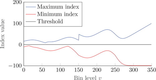
Interestingly, Figure 3 shows that the range of index values varies strongly. As a result, trial-and-error will be necessary to determine a threshold R that yields the desired throughput, if it exists. Moreover, Figure 3 suggests, by increasing the threshold R, that the system may end up in a situation where ${\max }_{w\in \mathcal{W}}\{\mathcal{\ell }(v_i)-\mathcal{\ell }(v_i+w)\}<R$ for each bin $i\in \mathcal{K}.$ So all arriving items will be rejected, and the target throughput will never be achieved. In order to prevent this situation and to set the throughput target directly, we propose to dynamically update the threshold. That is, let R_N denote the threshold value after having processed N items, then item N + 1 is accepted and assigned to $k^{*}$ if ${\mathcal{\ell }}^{*}\ge R_N,$ and rejected otherwise, and the threshold is updated as follows: (19) $$R_{N+1}=\{\begin{array}{cc}{R}_N-C_1·g(v_{k^{*}}+w)+C_2·(w-g(v_{k^{*}}+w)),\hfill & \mathrm{}\text{if}\mathrm{}{a}_{N+1}=k^{*},\hfill \\ R_N-C_1·w,\hfill & \mathrm{}\text{if}\mathrm{}{a}_{N+1}=0,\hfill \end{array}$$(19) where $a_{N+1}$ is the decision for item N + 1, and C₁ and C₂ are positive constants. Clearly, an item weight that contributes to the throughput is scaled by C₂ and increases the threshold, and an item weight that does not, is scaled by C₁ and decreases the threshold. Below we first heuristically argue how to choose the constants C₁ and C₂ such that the target throughput q is achieved. From (19) we readily obtain: $$R_N=R_0-C_1(w_N^g+w_N^r)+w_N^b{C}_2,$$ where R₀ is the initial threshold, and by substituting (9): (20) $$R_N=R_0-C_1(w_N-w_N^b)+w_N^b{C}_2.$$(20)

The total change in threshold value after N items is (21) $$\Delta R_N=R_N-R_0=-C_1(w_N-w_N^b)+w_N^b{C}_2.$$(21)

Normalizing $\Delta R_N$ by the total processed weight w_N, yields the threshold displacement per processed gram, which by substitution of (11), can be written as (22) $$\Delta {\overline{R}}_N=\frac{\Delta R_N}{w_N}=-C_1\frac{(w_N-w_N^b)}{w_N}+C_2\frac{w_N^b}{w_N}=-C_1(1-{\overline{w}}_N^b)+C_2{\overline{w}}_N^b.$$(22)

As $N\to \infty ,$ we obtain the long-term threshold displacement per processed gram: (23) $$\Delta \overline{R}=-C_1(1-{\overline{w}}^b)+C_2{\overline{w}}^b,$$(23) assuming that the limit ${\overline{w}}^b$ exists. Clearly, if $\Delta \overline{R}>0,$ then $R_N\to \infty$ as $N\to \infty$ and all items will be rejected, and if $\Delta \overline{R}<0,$ then $R_N\to -\infty$ and no items will be rejected. Hence, to be able to achieve the long-term target throughput $0<q<1,$ we have to impose $\Delta \overline{R}=0,$ yielding: (24) $$C_2=C_1\left(\frac{1}{{\overline{w}}^b}-1\right).$$(24)

The goal of the grader policy is to achieve the target throughput, ${\overline{w}}^b=q.$ So we set (25) $$C_1=C>0,\hspace{1em}{C}_2=C\left(\frac{1}{q}-1\right).$$(25)

If C₁ and C₂ satisfy (25), then we claim that, by using an index policy with threshold R_N updated according to (19), the throughput converges to the target q. To support this claim consider again (22). By substituting (25), we find that after N items have been processed: (26) $$\Delta {\overline{R}}_N=-C(1-{\overline{w}}_N^b)+C\left(\frac{1}{q}-1\right){\overline{w}}_N^b=C\left(\frac{{\overline{w}}_N^b}{q}-1\right).$$(26)

For the case where case ${\overline{w}}_N^b>q,$ it follows that $\Delta {\overline{R}}_N>0.$ As a result, the threshold increases and fewer items will be accepted. Similarly, if ${\overline{w}}_N^b<q,$ it follows that $\Delta {\overline{R}}_N<0.$ In this case the threshold decreases, such that more items will be accepted instead. In conclusion, if the throughput deviates from the target, the threshold updates will attempt to push it back.

To make this claim rigorous, note that the grader now evolves as a Markov chain with states $(v_1,\dots ,v_K,w,R)\in \mathcal{S}\times \mathcal{R},$ where $\mathcal{R}$ is the set of possible values for the threshold R. To obtain a countable set $\mathcal{R},$ we make the (mild) assumption that the target throughput q is a rational number. By (25), this implies that C₁ and C₂ are also rational, provided C is also chosen as a rational number, say $C_1=k_1/n$ and $C_2=k_2/n$ for some integers $k_1,k_2,n.$ Then $\mathcal{R}$ consists of all grid points $\dots ,-\frac{2}{n},-\frac{1}{n},0,\frac{1}{n},\frac{2}{n},\dots .$ Thus, the state space $\mathcal{S}\times \mathcal{R}$ is an infinite strip of grid points. The state transitions are specified by (1) and (19). Since ${\mathcal{\ell }}^{*}$ is bounded (as the weight distribution is finite), it follows that in states $(v_1,\dots ,v_K,w,R)$ with R sufficiently large, items are always rejected and transitions are directed to states with a smaller threshold. Thus, these states are transient. However, to prevent the Markov chain escaping to R = – ∞ (and no items will be rejected anymore), we have to satisfy a mean drift condition (Neuts, 1995) that states that the mean change of R in states $(v_1,\dots ,v_K,w,R)$ with R sufficiently small, is positive. More formally, the mean drift condition states that, if (27) $$\mathbb{E}[-C_1·g(V_{k^{*}}+W)+C_2·(W-g(V_{k^{*}}+W))]>0,$$(27) then the Markov chain on the infinite strip $\mathcal{S}\times \mathcal{R}$ is stable. In (27), the random variable W denotes the item weight and $V_{k^{*}}$ is the random content of the bin to which the item is allocated, in the finite Markov chain on $\mathcal{S}$ for the grader with no rejection. Substituting (25) into (27), we get (28) $$q<\frac{\mathbb{E}\left[W\right]-\mathbb{E}[g(V_{k^{*}}+W)]}{\mathbb{E}\left[W\right]}=1-\frac{\mathbb{E}[g(V_{k^{*}}+W)]}{\mu }.$$(28)

Note that the right-hand side corresponds to the long-term fraction of throughput weight for the grader with no rejection. Hence, for the Markov chain with a dynamic rejection threshold to be stable, the target q should be less than the maximal achievable throughput. If this Markov chain is stable, then indeed the limit ${\overline{w}}^b$ exists and $\Delta \overline{R}=0,$ from which we can conclude, by (23), that ${\overline{w}}^b=q.$ Summarizing, we proved the following result.

Theorem 4.

An index policy employing a rejection threshold that is dynamically updated according to (19) achieves target throughput q provided constants C₁ and C₂ satisfy (25) and q satisfies (28).

This approach to equip an index policy with a rejection threshold that is dynamically updated according to (19), is summarized in Algorithm 1, which will be referred to as index policy with Dynamic Rejection Threshold (DRT).

Algorithm 1.

Index policy with Dynamic Rejection Threshold (DRT).

Choose C > 0 and set C₁, C₂ according to (25). Initialize threshold R₀. Set N = 0 and repeat the following steps:

1. Determine the policy-optimal value ${\mathcal{\ell }}^{*}$ for item N + 1 with weight $w\in \mathcal{W}$. If ${\mathcal{\ell }}^{*}\ge R_N$ go to Step 2. Otherwise go to step 3.

2. Allocate item N + 1 to bin $k^{*}$. Empty this bin if $v_{k^{*}}\ge B$. Calculate $R_{N+1}$ according to Equation (19)(19) $$R_{N+1}=\{\begin{array}{cc}{R}_N-C_1·g(v_{k^{*}}+w)+C_2·(w-g(v_{k^{*}}+w)),\hfill & \mathrm{}\text{if}\mathrm{}{a}_{N+1}=k^{*},\hfill \\ R_N-C_1·w,\hfill & \mathrm{}\text{if}\mathrm{}{a}_{N+1}=0,\hfill \end{array}$$(19) . Set $N=N+1$. Return to step 1.

3. Reject item N + 1. Calculate $R_{N+1}$ according to Equation (19)(19) $$R_{N+1}=\{\begin{array}{cc}{R}_N-C_1·g(v_{k^{*}}+w)+C_2·(w-g(v_{k^{*}}+w)),\hfill & \mathrm{}\text{if}\mathrm{}{a}_{N+1}=k^{*},\hfill \\ R_N-C_1·w,\hfill & \mathrm{}\text{if}\mathrm{}{a}_{N+1}=0,\hfill \end{array}$$(19) . Set $N=N+1$. Return to step 1.

end.

The constant C scales the step size to adapt the rejection threshold. The larger C, the larger the average step size. The scheme proposed in Peeters et al. (2019) to dynamically adapt the threshold assumes a fixed constant C = 1. In Section 5, we will investigate through a simulation study the effect of the choice of C on the giveaway ${\overline{w}}^g,$ throughput ${\overline{w}}^b,$ and convergence to the target throughput q. For this study we investigate different index policies in addition to DRT.

5. Numerical results

In this section, we specifically aim to understand: (i) whether DRT can manage the throughput–giveaway trade-off; (ii) how DRT performs compared to the best known algorithms from practice and literature as well as MDP; and (iii) the impact of the production setting (target throughput, target weight, relative value of bulk batches) on the revenue. In order to address these points, we first describe the settings under which the experiments are performed. Then, we investigate the behavior of DRT through a numerical study performed in Matlab. In this study, the sensitivity of DRT to the scale parameter C is tested first. The best known algorithm in the literature is the Index Policy with Power function and Throughput target q (IPPT(q)) which is proposed in Peeters et al. (2019), which utilizes the differential policy of (13). We conduct a simulation study that compares DRT, IPPT(q) and MDP under different settings. Finally, we benchmark the revenue generated by using DRT against results provided by our industrial partner, and we study the impact of different production settings on the revenue.

5.1. Parameter and problem settings

The following settings are used in the numerical experiments. A discretized Normal distribution is used to generate product weights. That is, an item with weight w is sampled with probability $$p(w)=\frac{\varphi (w|\mu ,{\sigma }^2)}{\sum _{x=w_{\text{min}}}^{w_{\text{max}}}\varphi (x|\mu ,{\sigma }^2)},\hspace{1em}w\in \mathcal{W},$$ where $\varphi (x|\mu ,{\sigma }^2)$ is the density of the Normal distribution with mean μ and variance ${\sigma }^2.$ In all experiments we use μ = 100, σ = 15, $w_{\text{min}}=1,$ and $w_{\text{max}}=199.$ The discretized Normal distribution is denoted as ${\mathcal{N}}_D(\mu ,\sigma ).$ The grader uses K = 8 bins. Ásgeirsson (2014) showed that target weights that are (close to) a multiple of the mean item weight (for example, B = 300) generally yield low giveaway, and that the opposite is true for target weights that are far from a multiple of the mean item weight (such as B = 350). These cases are referred to as easy and hard, respectively. In the experiments we consider both easy and hard cases. Additionally, target throughputs in the range of zero through one are studied. Lastly, the relative value of bulk batches to retail batches per gram is based on practice, and typically ranges from 0.7 to 0.9. In the experiments, target weight, target throughput, and relative value of bulk batches are varied to illustrate the sensitivity of the performance in terms of revenue.

As mentioned in the previous section, we equip DRT with different index policies. In particular, we study IPP and PRE with the differential policy (13) or ratio policy (14). For each application of DRT we initialize $R_0=0.$ Furthermore, DRT in combination with an index policy has two important parameters: the scale parameter C and the parameters α and β in the loss functions (18) and (17) of IPP and PRE, respectively. For given value of C, α or β are tuned to minimize giveaway in A = 9 steps of the procedure described at the end of Section 4.1. In the next section we focus on how to tune the parameter C. In every simulation run, the order size Q is fixed at 10,000 batches, corresponding to a large customer order. In other words, items are generated until 10,000 batches are completed.

5.2. Parameter tuning

This section presents our findings regarding the impact of the scale parameter C in DRT. For expository purposes we have selected DRT in combination with IPP and a differential policy. Target weight B = 350, and target throughput q = 0.5 are used in the analysis². We investigate how ${\overline{w}}_N^b$ changes per item N. The results for the first N = 1000 items using $C={10}^{-4},{10}^{-5},$ and ${10}^{-6}$ are plotted in Figure 4.

Figure 4. Throughput after N items.

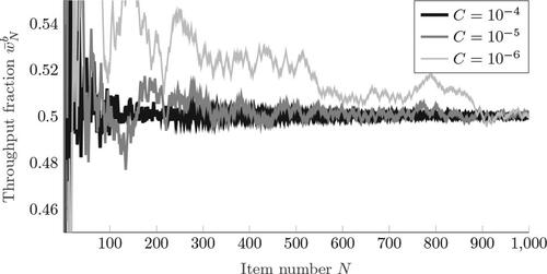
Figure 4 suggests that for all values of C the throughput approaches the target q = 0.5. Convergence is faster for larger values of C. Furthermore, Figure 5 shows that this behavior is caused by increased sensitivity of the threshold with respect to item allocations. Higher values of C result in higher variability of R_N. Most importantly, these figures suggest that DRT indeed approaches the target throughput q as N gets sufficiently large. So what prevents us from selecting an arbitrarily large value of C? This question is answered in Figure 6, which shows the absolute deviation from the target throughput $|{\overline{w}}_N^b-q|$ (Figure 6(a)) and giveaway ${\overline{w}}_N^g$ (Figure 6(b)) for different values of C and different policies. In particular, we study IPP and PRE with differential and ratio policies.

Figure 5. Value of threshold after N items.

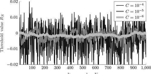
Figure 6. Sensitivity of various policies to C.

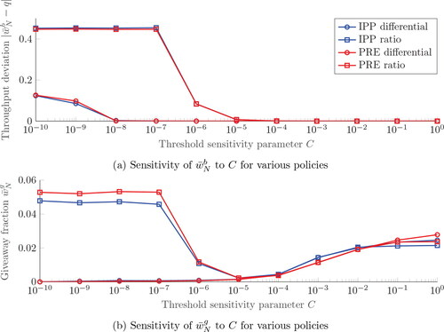
The data in Figure 6(a) presents a clear pattern, where DRT is no longer able to achieve the target throughput for small values of C. As observed in Figure 4, convergence to the target throughput is slower for smaller values of C, suggesting that there has been insufficient time for the algorithm to converge. As a result, for smaller order sizes, the minimal feasible value of C and corresponding giveaway should be larger. However, deviations from the target throughput occur much sooner for the ratio policies than the differential policies, as the range of values obtained for ratio policies is generally much greater. The disadvantage of ratio policies is further compounded by their poor giveaway performance for low values of C.

Instead, sensitivity of the giveaway of both differential policies is low from $C={10}^{-7}$ through $C={10}^{-5},$ where the deviation from the target throughput is small. We conclude that differential policies outperform ratio policies, with minimal difference between IPP and PRE. Due to their similar hallmarks, we proceed with DRT equipped with IPP utilizing a differential policy, although PRE appears equally suitable. In the following, we will simply refer to this combination of DRT and IPP as DRT. Finally, note that the value of the PRE differential policy for C = 1 corresponds to the peformance of the IPPT(q). We conclude that employing DRT leads to a substantial giveaway reduction of almost 2.4 percentage points when using $C={10}^{-7}$ with an IPP differential policy, illustrating the added value of DRT.

Based on these findings, we propose the following procedure to tune C. The idea is to set C as small as possible (for minimal giveaway), while still achieving the target throughput. The initial value of C is taken to be one, as Figure 6 suggests that this value achieves fast convergence to the target throughput. Subsequently, C is progressively decreased by division of 10 (to limit calculation time) as long as the permitted deviation δ from the target throughput is not violated. This procedure is used to conduct the remaining experiments, where tolerance δ is taken to be 0.1% of the target throughput q.

5.3. Numerical analysis of small-scale problems

In this section, we numerically explore the structure of the optimal policy for the single bin problem K = 1, and compare the performance of the DRT and IPPT(q) algorithms against the optimal solution produced by the MDP model.

5.3.1. Structural analysis

First, we consider a special case with K = 1 and no target throughput requirement, which has been studied in Section 3.3. The optimal policy is obtained by the value iteration algorithm (Puterman, 2014). For a specific problem instance with K = 1, B = 350 and normalized revenue of rejected weight $r_r=0.8$ per gram, Figure 7 shows the optimal actions in states (v, w). The closing-states (i.e., states (v, w) where v + w = B) have been marked white for clarity.

Figure 7. Optimal action per state $a^{*}(v,w)$ for K = 1, B = 350, and $r_r=0.8.$

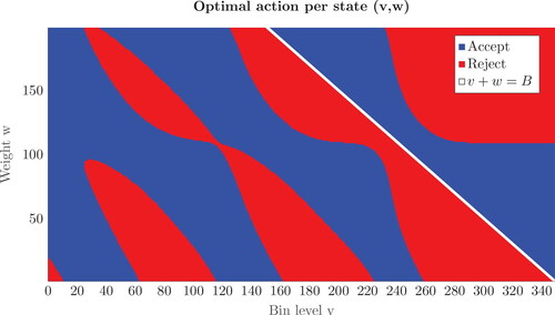
We observe from Figure 7 that optimal policies do not have a simple structure. Only in the area of closing-states (as marked white in Figure 7), do we see that the optimal policy is characterized by a switching curve. This insight aligns with Theorems 2 and 3. However, Figure 7 shows that optimal policies do not have a structure for non-closing-states. Therefore, Figure 7 illustrates that structural insights cannot be easily derived for non-closing states, even when we consider a special case with single bin and no throughput requirement. These observations also substantiate the analytical difficulty and practical challenges associated with our problem setting.

5.3.2. Performance of heuristics

Next, we benchmark DRT and IPPT(q) against the optimal solution obtained by the constrained MDP in Section 3.2. In addition, the solution (OPT) of the unconstrained MDP is determined to quantify the impact of the throughput constraint on the revenue. The constrained MDP is solved to optimality using LP solver in Matlab. and the unconstrained version is solved by value iteration. In order to keep the solution time tractable, a small-scale problem is considered.

We take K = 1, and the target weights and item sizes are scaled down with a factor 10 compared with the previously considered problem instances. Specifically, we consider batch sizes B = 30 and 35, and item weights $w\sim {\mathcal{N}}_D(10,1.5).$ The maximum and minimum item weights are taken to be $w_{\text{max}}=19$ and $w_{\text{min}}=\text{one}.$ respectively. Under these settings, the standard deviation of the discretized distribution deviates less than ${10}^{-8}$ from σ. Furthermore, both $r_r=0.7$ and 0.9 are considered. The target throughput is varied from q = 0 through q = 0.8 in steps of 0.1. A total of 10,000 batches are completed per parameter settings for both DRT and IPPT(q).

Figure 8 shows that the optimal revenue per gram is lower for the hard case B = 35 than for the easy one B = 30. Additionally, for all algorithms, the revenue is increasing in the target q, which is as expected, since batched weight (with little giveaway) is more valuable than rejected weight. Furthermore, the difference in revenue between the MDP solution and DRT is negligible, as it is less than 0.0022 in all cases. However, there is a significant gap between IPPT(q) and DRT, illustrating the impact of tuning the scale parameter C on the revenue.

Figure 8. Revenue per gram for $r_r=0.7,$ and B = 30 (left) and 35 (right).

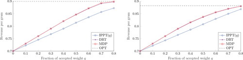
The second instance with higher value of rejected weight ($r_r=0.9$) is presented in Figure 9. We observe that the revenue curves are no longer strictly increasing and the fraction of accepted weight maximizing revenue is smaller than in Figure 8. Again DRT performs close to MDP, with the difference in revenue staying below 0.0026. For all algorithms, the revenue per gram is significantly higher than in case $r_r=0.7.$ For example, the gap in revenue between the MDP curves in Figures 8 and 9 ranges from 0.023 to 0.2. Lastly, it is concluded that DRT significantly outperforms IPPT(q) in all experiments.

Figure 9. Revenue per gram for $r_r=0.9,$ and B = 30 (left) and 35 (right).

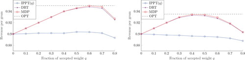
In conclusion, for small-scale problems, DRT results in near-optimal performance in all settings, and significantly outperforms IPPT(q) in terms of revenue. Next, we will study DRT in a case study.

5.4. Managerial insights: An industry case study

In this section, we perform experiments and case studies to provide insight for managers. Specifically, DRT is benchmarked against the algorithm currently used in practice to quantify the room for improvement. Insight into the trade-off between throughput and giveaway is obtained through additional experimentation. Lastly, sensitivity of the revenue with respect to different production settings in terms of flock, order, and revenue values are studied.

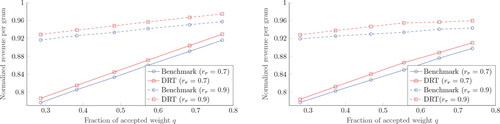
First, the performance of DRT is benchmarked in a practical setting. Our industrial partner provided us with simulation results of their state-of-the-art batcher. Algorithms currently used in practice are not capable of controlling the throughput, but solely control the fraction of items allocated. Hence, to get a fair comparison, the achieved throughputs from the benchmark case are used as target throughput in DRT. Additionally, DRT is tested with the item weight distribution and target weights from our industrial partner. In particular, for a grader with K = 8 bins, 10,000 items are generated using a ${\mathcal{N}}_D(100,15)$ distribution, varying the target throughput and using target weights B = 300 and 350, respectively.

DRT outperforms the benchmark in all settings. As shown in Figure 10, for the case B = 300, up to 0.015 more revenue per gram can be achieved. Also shown in Figure 10 is that for the case B = 350, the increase in revenue per gram ranges from approximately 0.01 to 0.02. To illustrate the impact of such a reduction, consider the following setting. A plant processes 15,000 broilers per hour for 16 hours per day. The plant is operational for 300 days per year, the average broiler weight processed is 1500 grams and the total fillet weight per broiler is 25% or 375 grams (Peeters et al., 2017), all broilers are processed into fillets, and the value of fillets is 4 Euro per kilogram. In such a case, an increase of 0.01 in the normalized revenue per gram represents a revenue increase of 1,080,000 Euro in fillets alone. This translates to yearly cost savings of between 750,000 and 2,270,000 Euro when using DRT over the benchmark. Moreover, implementation costs of DRT are relatively low, since only modifications in the allocation software are required.

Figure 10. Revenue per gram for the benchmark and DRT for B = 300 and 350.

Second, we study the relation between algorithm performance and the target weight. Figure 11 shows the giveaway of IPP without target throughput at different target weights after 10,000 bins are filled. The performance of IPP is used as baseline to generate target throughputs for the DRT algorithm, each of which are mentioned in the legend. Specifically, the target throughput of DRT is set to 75% and 50% of IPP throughput at each target weight, and the target weight is varied from 200 to 500 in steps of 10.

Figure 11. Giveaway per gram for different target weights.

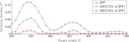
Figure 11 shows that, for all algorithms, the giveaway is relatively low for target weights that are a multiple of the mean item weight, and relatively high for target weights that are in between these values (illustrating the easy and hard cases). Furthermore, the overall level of giveaway decreases at higher target weights: more combinations of items can be made in larger bins, providing algorithms more flexibility to reduce giveaway. When the target throughput is lowered to 75% of the baseline, a significant giveaway reduction can be observed. DRT achieves close-to-zero giveaway around target weights that are a multiple of the mean product weight, as well as at target weights of 400 grams or higher. An additional giveaway reduction is achieved when only 50% of the baseline throughput is required, achieving negligible giveaway at all target weights except around B = 250. Figure 12 shows the corresponding revenue for $r_r=0.7$ and 0.9.

Figure 12. Revenue per gram for different target throughputs.

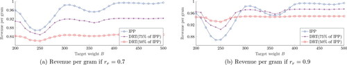
Figure 12 illustrates the revenue for different target throughputs. There is a strong relationship between revenue and normalized revenue of rejected weight. For $r_r=0.7,$ the baseline algorithm generates a higher revenue for all target weights. All algorithms obtain a relatively high revenue for target weights yielding low giveaway. When the value of rejected weight is increased to $r_r=0.9,$ a completely different picture is observed. Lower target throughputs (and thus more rejected weight) yield a higher revenue in cases where IPP yields high giveaway. Poultry plants have reported target weights towards the lower end of the studied setting. The potential gain in revenue for different throughput targets at these lower target weights strongly depends on r_r. For the case $r_r=0.7,$ a different production setting can yield up to 0.15 additional revenue per gram. For the case $r_r=0.9,$ this number changes to 0.06 per gram.

For plant managers, it is interesting to consider the above results in their production strategy. If their production setting changes, it is important to understand the ramifications in terms of revenue. Below, a number of different options and their impact on the revenue are discussed:

1. Suppose a customer demands batches with higher target weights B, which also corresponds to a higher throughput q. Figure 12(a) indicates that this change yields higher revenue if r_r is low, but Figure 12(b) shows that this potential gain strongly depends on how much B changes in case r_r is high.

2. Suppose the target throughput q is increased, because a customer demands more batches. The revenue increases if r_r is low (see Figure 12(a)), or if both r_r and the target weight B are high, as can be seen in the right part of Figure 12(b).

3. Suppose the target throughput is decreased, because a customer demands fewer batches. The revenue only increases if both r_r and giveaway are high, as indicated by Figures 11 and 12(b).

To conclude, DRT equipped with IPP converges to the target throughput in all cases presented, and yields low giveaway by tuning the scale parameter C. This indicates that DRT is capable of managing the throughput–giveaway trade-off well. Second, numerical experiments for small-scale problems show that the structure of the optimal policy is complicated and that DRT achieves near-optimal performance and significantly outperforms IPPT(q). Third, we have seen that DRT outperforms the algorithm currently used in practice in a wide range of realistic problem settings for the industry. Lastly, the revenue per gram of processed weight appears to be sensitive to the relative value of weight processed as bulk batches, target throughput, and target weight.

6. Conclusions and future work

This article studies a problem relevant to the poultry processing industry. Retail customers order batches with a given target weight for which they pay a fixed price, and impose a target throughput on poultry processing plants. Additional weight in these batches is not paid for by retailers, and thereby results in giveaway. Weight that is not used in making retail batches is rejected to a batching process that creates bulk batches, which are worth less per weight compared with retail batches. Operating under this target throughput, the goal of poultry processing plants is to maximize the revenue by minimizing the giveaway.

This problem is formulated as an MDP. In a special case of the problem with single bin and no throughput constraint, we derived structural results for states where item allocation immediately results in a filled bin. In particular, we identified that optimal policies have a switching-curve structure under certain conditions. Since the MDP model is computationally intractable for industry-sized problems, we introduced a new heuristic algorithm called DRT, using a dynamically updated rejection threshold.

The performance of DRT was investigated in a numerical study. For small-scale problems, DRT appeared to perform close to optimal. In addition, a case study was performed, where DRT was benchmarked against simulation results provided by our industrial partner. Numerical experiments showed a significant improvement under all studied settings. In particular, for a realistic setting obtained from our industry partner, numerical experiments anticipated a revenue increase of up to 2% (which translates to millions per year) through the use of DRT.

Using insights from the numerical analysis, managers will be able to identify their current production setting and make informed decisions about future changes. Specifically, when customers request changes in the production setting in terms of target weight, target throughput, or relative value of bulk compared with retail batches, managers will be able to identify and quantify the expected outcome. As a future work, it will be interesting to investigate whether DRT can be adapted to other optimization problems where rejection is an option, such as bin-packing or knapsack problems. As another direction for future research, machine learning models could be trained to predict the item weight distribution on a rolling horizon.

Acknowledgments

The authors thank the Department Editor and two anonymous referees for their constructive comments that helped significantly improve this article.

Additional information

Notes on contributors

Kay Peeters

Kay Peeters is a PhD student of the dynamics and control research group at the Eindhoven University of Technology. He holds an MSc degree in mechanical engineering from the same university. His PhD project is centered around the optimization of poultry processing plants, with a focus on control, planning, and design. His research interests include discrete-event simulation of manufacturing networks, production control and production scheduling.

Ivo J. B. F. Adan

Ivo J. B. F. Adan is a professor at the Department of Industrial Engineering of the Eindhoven University of Technology. His current research interests are in the modeling and design of manufacturing systems, warehousing systems and transportation systems, and more specifically, in the analysis of multi-dimensional Markov processes and queueing models.

Tugce Martagan

Tugce Martagan is an assistant professor and Marie S. Curie Research Fellow in the Department of Industrial Engineering at Eindhoven University of Technology. She received her PhD in industrial engineering from the University of Wisconsin-Madison. Her research interests include stochastic modeling and optimization of manufacturing systems.

Notes

1 When we relax our assumptions on special cases to capture other problem configurations, numerical experiments indicate that optimal policies are complex and do not exhibit a structural behavior.

2 These values are chosen based on production data obtained from our industry partners, and represent common industry practices.

References

- Ásgeirsson, A. (2014) On-line algorithms for bin-covering problems with known item distributions. Ph.D. thesis, Georgia Institute of Technology, Atlanta, GA.
- Asgeirsson, E. and Stein, C. (2006) Using Markov chains to design algorithms for bounded-space on-line bin cover, in Proceedings of the Meeting on Algorithm Engineering & Expermiments, Springer, New York, NY, pp. 75–85.
- Asgeirsson, E. and Stein, C. (2009) Bounded space online bin cover. Journal of Scheduling, 12(5), 461–474.
- Coffman Jr, E.G., Johnson, D.S., Shor, P.W. and Weber, R.R. (1993) Markov chains, computer proofs, and average-case analysis of best fit bin packing, in Proceedings of the Twenty-Fifth Annual ACM Symposium on Theory of Computing, Association for Computing Machinery, New York, NY, pp. 412–421.
- Correa, J.R. and Epstein, L. (2008) Bin packing with controllable item sizes. Information and Computation, 206(8), 1003–1016.
- Csirik, J., Johnson, D.S. and Kenyon, C. (2001) Better approximation algorithms for bin covering, in Proceedings of the Twelfth Annual ACM-SIAM Symposium on Discrete Algorithms, Society for Industrial and Applied Mathematics, USA, pp. 557–566.
- Derman, C. (1970) Finite State Markovian Decision Processes, Academic Press, Inc., Orlando, FL.
- Dósa, G. and He, Y. (2006) Bin packing problems with rejection penalties and their dual problems. Information and Computation, 204(5), 795–815.
- Manning, L. and Baines, R. (2004) Globalisation: A study of the poultry-meat supply chain. British Food Journal, 106(10/11), 819–836.
- Neuts, M. (1995) Matrix-Geometric Solutions in Stochastic Models: An Algorithmic Approach, Dover Publications, New York.
- OECD (2017, November) Meat consumption. Available at
- Peeters, K., Adan, I. and Martagan, T. (2019) Throughput control and giveaway minimization of a poultry product batcher, in 2019 Winter Simulation Conference, IEEE Press, Piscataway, NJ, pp. 2131–2141.
- Peeters, K., Martagan, T., Adan, I. and Cruysen, P. (2017) Control and design of the fillet batching process in a poultry processing plant, in 2017 Winter Simulation Conference, IEEE Press, Piscataway, NJ, pp. 3816–3827.
- Puterman, M.L. (2014) Markov Decision Processes: Discrete Stochastic Dynamic Programming, John Wiley & Sons, Hoboken, NJ.