The digital twin synchronization problem: Framework, formulations, and analysis

Abstract

As the adoption of digital twins increases steadily, it is necessary to determine how to operate them most effectively and efficiently. In this article, the digital twin synchronization problem is introduced and defined formally. Frequent synchronizations would increase cost and data traffic congestion, whereas infrequent synchronizations would increase the bias of the predictions and yield wrong decisions. This work defines the synchronization problem variants in different contexts. To discuss the problem and its solution, the problem of determining when to synchronize an unreliable production system with its digital twin to minimize the average synchronization and bias costs is formulated and analyzed analytically. The state-independent, state-dependent, and full-information solutions have been determined by using a stochastic model of the system. Solving the synchronization problem using simulation is discussed, and an approximate policy is proposed. Our results show that the performance of the state-dependent policy is close to the optimal solution that can be obtained with full information and significantly better than the performance of the state-independent policy. Furthermore, the approximate periodic state-dependent policy yields near-optimal results. To operate digital twins more effectively, the digital twin synchronization problem must be considered and solved to determine the optimal synchronization policy.

Keywords:

• Digital twins
• simulation
• production systems
• information update

1. Introduction

Following the adoption of new data communication and processing technologies in intelligent manufacturing, digital twins are considered one of the critical technologies in Industry 4.0 (Tao et al., 2019). One of the most common uses of a digital twin is monitoring a machine or a manufacturing system in real-time. However, they also allow us to predict the system’s future state by using simulation experiments that exploit the most recent information on the system state. The digital twin is also used to assist a decision with its predicted performance, also known in the literature as prescription. Monitoring, prediction, and prescriptions are some of the external services or functionalities provided by digital twins.

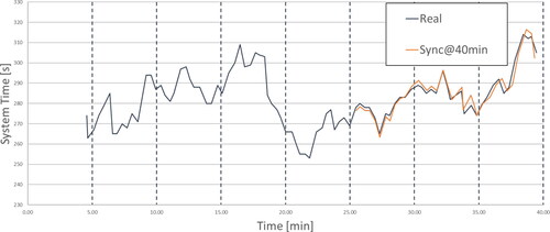
As data-collection and processing technology advances, the detail level of digital twins also increases to capture the dynamics of a manufacturing system with accuracy. A digital twin of a complex system, such as a manufacturing plant, may include thousands of variables that track the system dynamics. As the complexity of a digital twin increases, reflecting all the changes in the physical system in the digital twin, synchronizing the digital twin with the current status of the system, using the digital and to predict the system’s future performance, and using these predictions to make and revise decisions effectively become more challenging (Lugaresi and Matta, 2018). In particular, synchronizing all the variables with the data collected from the system, using the collected data to update the predictions, and using these predictions to make decisions take time, require more resources, and may affect the real-time operation of digital twins. On the other hand, not synchronizing a digital twin with the actual state of the physical system may lead to inaccurate predictions, especially in highly dynamic contexts. Figure 1 shows an example of a digital twin that predicts the system time in a production facility while synchronizing with the real system. While synchronizing a digital twin will improve its predictive capability into the future, the costs related to retrieving and processing data, updating models, obtaining predictions, and updating decisions must be compared with the benefits arising from an improved prediction. A method must be developed to make an operational decision to determine when and how to synchronize a digital twin to balance these costs.

Figure 1. An example of synchronization executed in real time; synchronization frequency is 40 minutes. The values represented in the graph are the system time of parts processed in a production system: measured from the physical system (blue) and predicted by the digital twin (red) since the 25th minute.

This study defines and analyzes the optimal synchronization problem as a dynamic stochastic control problem. Since synchronization can involve multiple decisions, different variants of the synchronization problem are discussed. The objective of the control problem is to minimize the expected total cost of synchronizing the digital twin and the total misalignment costs caused by the prediction error due to not synchronizing the digital twin in a given period. We focus on the digital twin synchronization problem for a manufacturing system. In this setting, the number of parts produced in a given time interval by a production system that observes downtime will be lower than when the system is up and running. If the digital twin is used as a simulation tool to predict the daily resource requirements that depend on daily production, the production system must be simulated again. Simulating the system again requires initializing the simulation model with the current state of the production system. We formulate the problem as a stochastic optimal control problem that minimizes the expected synchronization and bias costs by determining when to synchronize and when not to synchronize the digital twin based on the observation of the state of the production system. By formulating the problem as a stochastic nonlinear integer program, we determine the state-dependent and state-independent policies using a scenario approach. We also discuss how the synchronization problem can be solved using simulation and propose an approximate policy. The performances of the state-dependent, state-independent, approximate, and full-information policies are compared.

The organization of the remaining part of this article is as follows. The pertinent literature is reviewed in Section 2. Section 3 discusses the different forms of synchronization that can be relevant in real applications. The optimal digital twin synchronization problem is introduced and defined formally for the general case in Section 4. The optimal digital twin synchronization problem for an unreliable production system is given in Section 5. The solution to the synchronization problem using simulation is discussed in Section 6. The exact analytical solution of the optimal digital twin synchronization problem for an unreliable production system that yields the state-independent, state-dependent, and full-information policies is obtained by using a scenario approach, and an approximate synchronization policy is proposed in Section 7. Numerical results that analyze the effect of system parameters on the performance of the state-independent and state-dependent policies are given in Section 8. Finally, the conclusions are provided in Section 9.

2. Literature review

The tradeoff between acquiring more information for decision-making and acting with the existing information has been discussed in different settings (Moore and Whinston, 1986; Ballou and Pazer, 1995). We focus our review on studies addressing this problem in simulation and digital twins. In the simulation literature, Sargent (2013) states that increasing confidence in a model has a diminishing return on the value obtained from that model. Similarly, in the digital twin synchronization problem, synchronizing the digital twin more frequently increases the confidence in a simulation model, but at a cost. The additional cost of synchronizing a digital twin may not be justified if the benefits of improving the predictions are limited.

In the context of digital twins, synchronization may burden the communication network. Modoni et al. (2019) acknowledge that a high frequency and detailed synchronization can entail a significant processing cost, and proper balancing should be pursued. In Kuts et al. (2019), experiments are run in a manufacturing laboratory demo center to test a synchronization Internet–of–Things (IoT) architecture; a criterion of evaluation is the ping time in the network communications. With a similar purpose, Ait-Alla et al. (2019) study the impact of positioning more sensors on the communication speed between physical and digital systems. Jia et al. (2021) explore the clock synchronization problem in industrial IoT systems and consider network resource consumption as a critical criterion for assessing and validating synchronization algorithms. In Hashash et al. (2022), near-zero latency is indicated as a significant criterion for sustaining high quality–of–service for dynamic digital twins operating in variable environments. An upper limit value for the maximum time allowed for the data synchronization task is considered in the demonstration reported in Manothiang and Nuratch (2021). Summarizing from this first stream of work, the containment of the synchronization frequency is expected to help decrease resource network consumption, latency, and communication failures.

The prediction of a digital twin can differ from the behavior of a physical system, and de-synchronization may affect the quality of the prediction. Gao et al. (2021) present an anomaly detection framework for monitoring the different behavior between digital twin and physical system due to modeling errors and sensor and faults in the physical system. This difference may lead to additional problems when digital twins are used for different decisions. Hanisch et al. (2005) define the online simulation initialization problem that focuses on aligning system variables with the available data. Zipper and Diedrich (2019) specify an optimization problem to synchronize the states of the digital twin with the physical system and detect changes; the objective is the minimization of the error between measurements from a physical system and predictions from its digital twin. Zipper (2021) presents an extension of the state synchronization methodology to synchronize online simulations in real-time. Zipper and Diedrich (2019) and Zipper (2021) focus on the digital twin of a physical resource that has an analytical model that can be used to evaluate its performance in a deterministic way. In Hashash et al. (2022), the authors present a dual objective optimization problem to minimize the loss function between the simulation of an autonomous vehicle traversing a dynamic environment obtained by a deep neural network at the wireless network edge and the physical twin. The tradeoff between the accuracy obtained by training the model again and the time that will be used to train the model is addressed in this study. Lengerke et al. (2022) present a goal-oriented communication approach to decide when to synchronize subject to traffic control and probabilistic synchronization performance constraints to balance the tradeoff between the additional data traffic generated by more frequent synchronizations and the accuracy. A different synchronization problem has been presented by Qin et al. (2022), in which the authors deal with the alignment of robot manipulations in robot-assisted surgeries.

Synchronizing digital twins with their respective physical systems may involve updates of the simulation models used for predictions. Cardin and Castagna (2011) discuss different operational problems when digital twins are used as a forecasting tool for production planning. Model inaccuracies can be caused by inadequate model level or because the physical system is generally an asset with a long life cycle that is inevitably prone to changes. In Müller et al. (2022), the data sources from physical and digital twins are compared to detect anomalies. In Negri et al. (2021), the authors propose a framework for production scheduling using the last data collected from the field but they do not consider the synchronization problem.

Another stream of literature dealing with synchronization focuses on the IoT architecture. In Manothiang and Nuratch (2021), the authors focus on a detailed architecture that includes 3D equipment models. They show that data communication between their physical and digital systems can be completed in milliseconds.

This study follows our preliminary work where the digital twin synchronization problem was defined, and a stylistic problem of predicting the number of successes in a given number of binomial trials was used to discuss different synchronization policies (Tan and Matta, 2022). Our study differs from the previous studies in terms of the setting used and in terms of the methodology used. We focus on a digital twin of a manufacturing system that is primarily used to predict its future performance. Unlike the synchronization problem for a digital twin that monitors a machine, a discrete-event simulation that captures the interaction among different entities is used to predict its future performance. The performance of a manufacturing system is significantly affected by random events, such as machine failures, random processing time, or random arrivals. As a result, even if the digital twin uses a correct model to represent the physical system, synchronization may be necessary to make the digital twin follow the physical system’s random trajectories. Therefore, the synchronization problem is related to increasing the accuracy of the predictions by using more frequent synchronizations without neglecting their related costs.

The contribution of this article is 2-fold. First, the optimal digital twin synchronization problem, with its variants, for a manufacturing system is formally defined as a stochastic control problem. Second, the optimal digital twin synchronization problem for a specific unreliable production system is solved analytically to explain the problem and its solution in detail. The solution to the synchronization problem by using simulation is also discussed. The state-independent and state-dependent policies are determined exactly and compared with the optimal solution obtained with full information and an approximate policy. It is shown that the state-dependent policy significantly improves the performance compared with the state-independent policy and yields an average cost close to the one that can be obtained with the full information. Furthermore, the proposed approximate policy delivers a near-optimal performance.

3. Synchronization problems

To use the primary services provided by the digital twin effectively, the digital system and the physical system need to be kept aligned. There can be various reasons for the misalignment between the digital and physical systems. First, the randomness intrinsic in the physical processes may cause deviations of the digital twin from the real system trajectory. A second reason is related to the evolution of the physical system. Indeed, manufacturing systems have a long life cycle in which many changes are introduced to improve system efficiency, match customer demand, etc. In addition, equipment may degrade over time. Therefore, upon a system change (natural or artificial), the digital twin starts deviating from its real twin, and a model update is necessary. Lastly, it may happen that the digital twin is using models that are not fully representative of the physical system. In this case, a model update is necessary.

According to the literature described in the previous section, in particular (Gao et al., 2021; Hashash et al., 2022; Lugaresi and Matta, 2018; and Modoni et al., 2019) synchronizing a digital twin may involve several activities ranging from retrieving the system state to updating the action prescribed by the digital twin. State retrieval is an activity always needed when a synchronization task is executed. Indeed, an alignment of the digital twin must know entirely or partially the system state. Therefore, every form of synchronization problem includes a state update activity that transfers the system state from physical to digital. Further, the system can be partially observable, and some tasks might be executed to build an estimate of the current state of the physical system. Predictions from a digital twin are continuously compared with measurements from the system, when available. The performance estimates are renewed every time synchronization occurs by launching a new prediction calculation. If deviations are detected from the comparison, an update of either the digital model logic or its parameters could be necessary to realign the twins. Furthermore, the prediction and the prescription may need to be updated upon a disruptive event. All these activities require an effort in terms of time needed for their execution and data communication flow.

The most straightforward synchronization problem is the prediction update problem, which aims at deciding when to execute a new simulation experiment to obtain an updated estimate of the performance of the digital twin. Table 1 gives a list of the synchronization problems discussed in this section. Depending on the detail level of the digital model and the complexity of the system, obtaining a new prediction may involve a significant amount of time. When a simple digital twin, e.g., a digital twin of an electric motor, is used, the time for generating a new prediction is very short (less than a second). On the contrary, this time can be large for complex systems that require detailed simulation, such as the case for estimating the lead time in semiconductor manufacturing systems. In these cases, deciding when to simulate becomes relevant because the new prediction must be available before the decision epoch. The activities included in this type of synchronization are the state update and the simulation experiment for the prediction.

Table 1. Relevant synchronization problems

Problem	Activities				Decisions
	State	Prediction	Model	Prescription
Prediction update	●	●			When to provide a new prediction
Model update	●	●	●		When to modify the digital twin model
Prescription update	●	●		●	When to provide a new decision
Synchronization problem	●	●	●		When to modify the digital twin model and update the prediction
General synchronization problem	●	●	●	●	When to modify the digital twin model, update the prediction and the decision

All the activities are updates of different components (state, prediction, model, prescription) and require effort. Prediction update and model update are single-type decision problems. Synchronization and general synchronization problems are joint decision problems. All problems are dynamic in a multi-stage time horizon setting.

Another problem often discussed in the literature is the realignment of the model used by the digital twin for generating the prediction referred to as the model update problem in Table 1. The model update may involve only updating its parameters or increasing the detail level of the model and determining its parameters by using the most recent observations from the physical system. Indeed, when a significant enough deviation of the prediction from the measured performance is detected, a model change is needed, or simply changing an inadequate model topology. The deviation can be caused by several reasons, such as modification of the physical system, having insufficient detail level of the model, or using parameters estimated from old data. The changes can be related to the model logic, the parameters used in the model, or both. The activities to be included in this type of synchronization are the state update, the model update, and the prediction update. The prediction update may be needed because the last available prediction is likely to be invalid. Frequent changes in the model may cause instability of predicted performance, explainability issues for decision-makers, unavailability of prediction service, and network communication issues. A rarely updated model can still be valid in static environments but not adequate in dynamic ones.

The prescription update problem has extensively been discussed in the decision-making literature. In the context of decisions assisted by digital twins, a prescription has to be considered as a decision. The action to update a decision must be evaluated together with the decision of re-obtaining a new prediction because the last can decrease the error and possibly improve the decision. Thus, this problem defines when to update the prediction and when to update the decision. The activities to be included in this type of synchronization are the state update, the prediction update, and the prescription update.

The most treated problem in the literature is the update of the model and the prediction. For this reason, when we refer to this problem in this work, we use the name synchronization problem. However, the reader must be aware that the same terms are used in the literature indistinctly also for the other different problems shown in Table 1. This problem defines when to update the model and provide a new prediction, whereas the prescription decision is not considered. The activities to be included in this type of synchronization are the state update, the prediction update, and the model update. The extension of this problem is reported in Table 1 as the general synchronization problem and also includes the prediction update. To the best of our knowledge, this problem has not yet been addressed in the literature.

4. Optimal digital twin synchronization problem

Following the framework in Section 3, we now present a general formulation of the synchronization problem. Considering the scope of the general synchronization problem depicted in Table 1, the objective of the optimal digital twin synchronization problem is finding an optimal policy that determines when to update the predictions obtained by the digital twin, when to update the digital twin model, and when to update the decision at each decision epoch based on the observed state of the system.

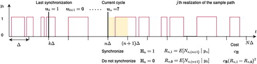
Figure 2 shows a sample evolution of the next period’s resource requirements (R_n,1 and R_n,0) that is used as the primary performance measure of an unreliable production system tracked by a digital twin and the synchronization decisions given at every Δ cycles (${\mathrm{H}}_n$) depending on the state of the station (y_n). In this example, only the prediction synchronization problem is depicted. The optimal digital twin synchronization problem yields a policy that determines when to synchronize and when not to synchronize, depending on the state of the system at a given time. We define this illustrative synchronization problem formally in Section 5, discuss its solution using simulation in Section 6, and solve it optimally in Section 7.

Figure 2. The decisions, state variables, and costs associated with the synchronization decision of an unreliable station for a given sample path.

4.1. Physical system description

The physical system evolves stochastically with discrete time $t=0,1,\dots .$ The system is evaluated every Δ times intervals. The performance measure at time $n\Delta$ is a random variable denoted with R_n. Assuming that we are at the nth evaluation at time $n\Delta ,$ we are interested in predicting the expected performance at time $\tau \Delta ,\mathbb{E}[R_{\tau }]$ within the interval $n\Delta <\tau \Delta \le (n+\delta )\Delta$ as well as the expectation of other functions that depend on the system performance measure at time $\tau \Delta .$ The parameter δ is given and can be considered as the forecasting horizon.

The observed system state at time $k\Delta$ is y_k. For the general case, y_k can be a multidimensional tuple of discrete and continuous values. The tuple of observed system states available at time $n\Delta$ with the last observation at time $k\Delta ,$ k < n is depicted with the tuple ${\mathbf{y}}_{n,k}=(y_0,y_1,\dots ,y_k).$ Then the full history of the system states at time $n\Delta$ is ${\mathbf{y}}_{n,n}.$ The expected value of the performance measure given the full history is $\mathbb{E}[R_{\tau }|{\mathbf{y}}_{n,n}].$

4.2. Digital system description

A digital twin is available to calculate the predicted system performance numerically. The predicted system performance at time $\tau \Delta$ is denoted with ${\widehat{R}}_{\tau }.$ In this work, the digital twin is a discrete-event simulation model that represents the system dynamics relevant for estimating the key performance of the physical system. Since the physical system is stochastic, the simulation model is also stochastic. The simulation model is executed to predict system performance, such as production throughput, inventory levels, resource utilization, system time, service levels, etc. Due to the physical system’s stochastic behavior, the digital twin may become misaligned from the physical system, thus jeopardizing its prediction capabilities. This section presents the model of the digital twin used to decide when synchronizing digital and physical systems.

The simulation model is developed at a certain detail level d, where higher values correspond to more detailed models and adequacy to the physical system. Simulation input parameters are fitted based on real observations of the variables that are modeled in a stochastic way in the simulation model. Examples of such variables are part arrivals, failure events, processing times, etc. The set of the fitted input simulation parameters is denoted with p. When modifying the detail level and the parameters of the digital twin are considered, the detail level and the parameters at time $n\Delta$ are denoted with d_n and ${\mathbf{p}}_n,$ respectively.

The digital twin is a simulation program run at initial time 0 and evaluated at time instances $\Delta ,2\Delta ,\dots ,k\Delta ,\dots ,n\Delta .$ The state of the digital twin at time $n\Delta$ before the action at time $n\Delta$ is taken includes the available history of the physical system states ${\mathbf{y}}_{n,k}$ and the state of the digital twin model with its detail level d_n and parameters ${\mathbf{p}}_n.$ That is ${\mathbf{S}}_n=({\mathbf{y}}_{n,k},d_n,{\mathbf{p}}_n).$

The performance of the system at time $\tau \Delta$ predicted by simulation is a function g that depends on the values of the observations of the performance measures, the physical system states last synchronized at time $k\Delta ,k\le n,$ i.e., ${\mathbf{y}}_{n,k},$ the current digital twin model with its detail level and parameters, and the prediction interval. This estimate is denoted with function $g(\tau ,{\mathbf{y}}_{n,k},d_n,{\mathbf{p}}_n),$ i.e., $\mathbb{E}[{\widehat{R}}_{\tau }|{\mathbf{S}}_n]=g(\tau ,{\mathbf{y}}_{n,k},d_n,{\mathbf{p}}_n).$

Since the digital twin is not a perfect representation of the actual system, the prediction obtained by using the digital twin is not equal to the prediction that can be obtained by using the full history of physical system states, i.e., $\mathbb{E}[{\widehat{R}}_{\tau }|{\mathbf{S}}_n]\ne \mathbb{E}[R_{\tau }|{\mathbf{y}}_{n,n}].$ Another cause of prediction error is the inability to use all the information available on the actual performance until time $\Delta n.$ Indeed, as the digital twin uses new information, the model’s parameters are updated with the new information, and the detail level of the model is increased, the prediction is expected to improve. Therefore, to improve the accuracy of performance prediction made at time $n\Delta ,$ it is possible to synchronize simulation with the real system by updating the predictions by collecting y_n and using ${\mathbf{y}}_{n,n}$ or by modifying the model by increasing its detail level and/or updating its parameters with ${\mathbf{y}}_{n,n}$.

4.3. Actions

At each observation epoch, three different decisions need to be given: setting the detail level of the digital twin model, deciding whether to update its parameters with the most current observed data, and deciding whether to update the predictions.

The decision at time $n\Delta$ is given by ${\mathbf{u}}_n=({\mathrm{H}}_n,d_n,{\mathbf{p}}_n)$ where ${\mathrm{H}}_n$ is the prediction update decision that has a value of one if the prediction update decision is taken and zero otherwise, d_n is the detail level of the digital twin, and ${\mathbf{p}}_n$ is its parameters that will be used for running the digital twin following the decision at time $n\Delta .$ The set of decisions taken from time 0 until $n\Delta$ is given in the tuple ${\mathbf{\chi }}_n=({\mathbf{u}}_0,{\mathbf{u}}_1,\dots ,{\mathbf{u}}_{n-1}).$

At a given time, if a parameter update decision is taken, the current state of the physical system will be retrieved to determine the parameters with the current observation. The same values are then also used to update the predictions, i.e., ${\mathrm{H}}_n=1.$ Similarly, suppose it is decided to increase the detail level of the digital twin. In that case, the current state of the physical system will be retrieved, and the parameters of the model will be determined based on the updated detail level. The parameter update and the detail level increase decisions are parts of the model update decision.

Given that the predictions have been synchronized at time $k\Delta ,$ at time $n\Delta >k\Delta ,$ the detail level has been changed at time $l\Delta ,$ and the parameters are updated at time $m\Delta ,n\Delta >l\Delta >m\Delta$ if a synchronization action is not taken at time $n\Delta ,$ that is if the predictions are not updated, the detail level of the model is not modified, and its parameters are not updated, the state of the digital twin does not change, i.e., ${\mathbf{S}}_{n+1}={\mathbf{S}}_n=({\mathbf{y}}_{n,k},{\mathrm{d}}_l,{\mathbf{p}}_m)=((y_0,y_1,\dots ,y_k),{\mathrm{d}}_l,{\mathbf{p}}_m).$

The prediction update action at time $n\Delta$ adds all the observations since the last synchronization of the system at time $k\Delta ,$ ($y_{k+1},y_{k+2},\dots ,y_n$) to the synchronization history. That is ${\mathbf{y}}_{n,n}=(y_0,y_1,\dots ,y_n)$ is used to make the prediction. The parameter update decision uses ${\mathbf{y}}_{n,n}$ to determine the updated values of the parameters ${\mathbf{p}}_n.$ Therefore, when the parameter update decision is taken, ${\mathbf{p}}_n\ne {\mathbf{p}}_m.$ The model-detail-level-increase decision modifies the logic of the digital twin to d_n and updates its parameters. Therefore, when the model-detail-level-increase decision is taken, d_n > d_l and $d_n\ne d_l.$ Since the additional information can only be used to improve the accuracy and is ignored otherwise, the system’s accuracy cannot degrade with a synchronization action. With the new observation, the prediction of the expected value of the performance measure at time $\tau \Delta ,n\Delta \le \tau \Delta \le (n+\delta )\Delta$ can be updated, and the bias of the estimated performance will likely be reduced. However, this reduction is likely to decrease as τ increases.

The state ${\mathbf{S}}_{n+1}$ at time $(n+1)\Delta$ is determined based on the previous state ${\mathbf{S}}_n$ and on the action ${\mathbf{u}}_n=({\mathrm{H}}_n,d_n,{\mathbf{p}}_n)$ taken at time $n\Delta$: (1) $${\mathit{S}}_{n+1}=S^{\mathrm{M}}({\mathit{S}}_n,{\mathit{u}}_n)=\{\begin{array}{cc}((y_0,y_1,\dots ,y_k,\dots ,y_n),d_l,{\mathbf{p}}_m)\hfill & ({\mathrm{H}}_n=1,d_n=d_l,{\mathbf{p}}_n={\mathbf{p}}_m)\hfill \\ ((y_0,y_1,\dots ,y_k,\dots ,y_n),d_l,{\mathbf{p}}_n)\hfill & ({\mathrm{H}}_n=1,d_n=d_l,{\mathbf{p}}_n\ne {\mathbf{p}}_m)\hfill \\ ((y_0,y_1,\dots ,y_k,\dots ,y_n),d_n,{\mathbf{p}}_n)\hfill & ({\mathrm{H}}_n=1,d_n>d_l,{\mathbf{p}}_n\ne {\mathbf{p}}_m)\hfill \\ ((y_0,y_1,\dots ,y_k),d_l,{\mathbf{p}}_m)\hfill & ({\mathrm{H}}_n=0,d_n=d_l,{\mathbf{p}}_n={\mathbf{p}}_m)\hfill \end{array}$$(1) where $S^{\mathrm{M}}$ denotes the transition function. In Equation (1)(1) $${\mathit{S}}_{n+1}=S^{\mathrm{M}}({\mathit{S}}_n,{\mathit{u}}_n)=\{\begin{array}{cc}((y_0,y_1,\dots ,y_k,\dots ,y_n),d_l,{\mathbf{p}}_m)\hfill & ({\mathrm{H}}_n=1,d_n=d_l,{\mathbf{p}}_n={\mathbf{p}}_m)\hfill \\ ((y_0,y_1,\dots ,y_k,\dots ,y_n),d_l,{\mathbf{p}}_n)\hfill & ({\mathrm{H}}_n=1,d_n=d_l,{\mathbf{p}}_n\ne {\mathbf{p}}_m)\hfill \\ ((y_0,y_1,\dots ,y_k,\dots ,y_n),d_n,{\mathbf{p}}_n)\hfill & ({\mathrm{H}}_n=1,d_n>d_l,{\mathbf{p}}_n\ne {\mathbf{p}}_m)\hfill \\ ((y_0,y_1,\dots ,y_k),d_l,{\mathbf{p}}_m)\hfill & ({\mathrm{H}}_n=0,d_n=d_l,{\mathbf{p}}_n={\mathbf{p}}_m)\hfill \end{array}$$(1) , the first transition corresponds to the prediction update decision, the second corresponds to the parameter update decision, the third depicts the model-detail-level-increase decision, and the last is the no synchronization decision.

4.4. Costs

Each synchronization action has a cost that increases proportionally with the time and resources used to align the digital twin with its physical counterpart. Cost increases when the detail level of the digital twin is increased, and its parameters are updated. The total digital twin cost of action ${\mathbf{u}}_n=({\mathrm{H}}_n,d_n,{\mathbf{p}}_n),$ is (2) $$C_{\text{DT}}({\mathbf{u}}_n)=f({\mathrm{H}}_n,d_n,{\mathbf{p}}_n)$$(2) where $f(·)$ is an increasing function of ${\mathrm{H}}_n,$ d_n, and ${\mathrm{I}}_{\{{\mathbf{p}}_n\ne {\mathbf{p}}_m\}}$ and ${\mathrm{I}}_x$ has a value of one if condition x is satisfied and zero otherwise.

The cost of increasing the detail level is expected to increase as d_n approaches one, and a fixed cost of parameter update cost is expected to be incurred if ${\mathbf{p}}_n\ne {\mathbf{p}}_m$ (Sargent, 2013). Furthermore, the cost of updating the predictions is lower than the cost of updating the parameters of the digital twin, and the cost of updating the parameters is lower than the cost of increasing its detail level.

The cost related to the prediction bias for the prediction at time $\tau \Delta$ is denoted with $c_{\mathrm{B}}(\tau ,{\mathbf{S}}_n,{\mathbf{u}}_n).$ This cost depends on the difference between the expected value of the performance measure at time $\Delta \tau$ (with $(n+1)\Delta \le \tau \Delta \le N\Delta$) obtained by using the full history at time $n\Delta$ in the most detailed digital twin, and the performance measures obtained with the digital twin following the synchronization decision.

The prediction bias cost related to the synchronization decision at time $n\Delta$ for the period $\tau >n$ is assumed as follows: (3) $$C_{\mathrm{B}}(\tau ,{\mathbf{S}}_n,{\mathbf{u}}_n)=h\left(\mathbb{E}\left[R_N\right|{\mathbf{y}}_n],g(\tau ,{\mathbf{y}}_{n,k},d_n,{\mathbf{p}}_n)\right)$$(3) where function $h(·)$ is a convex function. To calculate the bias cost, an estimate of $\mathbb{E}[R_{\tau }|{\mathbf{y}}_{n,n}]$ can be obtained from the available history or by using the digital twin. Function $g(\tau ,{\mathbf{y}}_{n,k},d_n,{\mathbf{p}}_n)$ can be obtained by using the digital twin.

The synchronization action costs can be set depending on the relative accuracy improvement to be obtained with a synchronization action that requires a particular level of resource to be used.

4.5. The optimal synchronization problem

The main problem considered in the general synchronization problem is deciding whether to update the predictions by using the current observations of the real system, whether to update the parameters of the digital twin, and whether to increase its detail level. The decision can be taken at any time epoch until N and balances the tradeoff between the bias of the prediction and the total costs incurred to make the prediction.

The objective is finding a policy Π that sets the decision variables ${\mathbf{u}}_n$ based on the observed state variables ${\mathbf{S}}_n,$ i.e., ${\mathbf{u}}_n=U^{\Pi }({\mathbf{S}}_n)$ to minimize the expected cumulative cost of prediction bias and of synchronizations: (4) $$\underset{{}_{\Pi }}{\mathrm{\text{min}}}\sum _{n=0}^N{C}_{\text{DT}}(U^{\Pi }({\mathbf{S}}_n))+\mathbb{E}[C_{\mathrm{B}}(S^{\mathrm{M}}({\mathbf{S}}_n,U^{\Pi }({\mathbf{S}}_n))\left|{\mathbf{S}}_0\right]$$(4) where the cost functions are defined with Equations (2)(2) $$C_{\text{DT}}({\mathbf{u}}_n)=f({\mathrm{H}}_n,d_n,{\mathbf{p}}_n)$$(2) and (3)(3) $$C_{\mathrm{B}}(\tau ,{\mathbf{S}}_n,{\mathbf{u}}_n)=h\left(\mathbb{E}\left[R_N\right|{\mathbf{y}}_n],g(\tau ,{\mathbf{y}}_{n,k},d_n,{\mathbf{p}}_n)\right)$$(3) , and Equation (1)(1) $${\mathit{S}}_{n+1}=S^{\mathrm{M}}({\mathit{S}}_n,{\mathit{u}}_n)=\{\begin{array}{cc}((y_0,y_1,\dots ,y_k,\dots ,y_n),d_l,{\mathbf{p}}_m)\hfill & ({\mathrm{H}}_n=1,d_n=d_l,{\mathbf{p}}_n={\mathbf{p}}_m)\hfill \\ ((y_0,y_1,\dots ,y_k,\dots ,y_n),d_l,{\mathbf{p}}_n)\hfill & ({\mathrm{H}}_n=1,d_n=d_l,{\mathbf{p}}_n\ne {\mathbf{p}}_m)\hfill \\ ((y_0,y_1,\dots ,y_k,\dots ,y_n),d_n,{\mathbf{p}}_n)\hfill & ({\mathrm{H}}_n=1,d_n>d_l,{\mathbf{p}}_n\ne {\mathbf{p}}_m)\hfill \\ ((y_0,y_1,\dots ,y_k),d_l,{\mathbf{p}}_m)\hfill & ({\mathrm{H}}_n=0,d_n=d_l,{\mathbf{p}}_n={\mathbf{p}}_m)\hfill \end{array}$$(1) describes the transition equations.

To solve this problem, a digital twin estimates the expected bias cost for different control actions by calculating the bias cost for different sample paths. At each period n, the history of observations, together with the digital twin, is used to have an estimate of the expected value of the performance measure $\mathbb{E}[R_{\tau }|{\mathbf{y}}_{n,n}].$

In addition to the functional parameters that specify the synchronization and bias costs, this problem uses a digital twin that provides the predictions of the performance measure based on the available state information and the history of system observations as the model inputs and yields the optimal synchronization policy as its output.

With the exogenous random process given for the evolution of the performance measure of the physical system, this problem can be analyzed as a sequential decision-making problem by using different approaches, including reinforcement learning (Powell, 2021). This is a challenging problem since the evolution of the performance measure of the physical system, as well as the effect of the synchronization actions on the accuracy improvement, need to be learned and updated with the new information starting with the prior estimates.

5. Digital twin synchronization of a production system

We now present the problem of synchronizing an unreliable production system’s digital twin to decide whether to update the predictions by using the current observations to explain the synchronization problem and discuss its solution.

5.1. Problem description

The following example explains the problem to be analyzed in this section: a production system that produces one part every hour is observed every morning to predict the resource requirements for a 10-h day. Depending on the prediction of the number of parts to be produced in the next 10 h, the resource requirements, such as the number of workers, are revised. If the output of the production system was not affected by any failures, i.e., if the production system were reliable, 10 parts would be produced during this day and the resource requirements would be set without considering a possible deviation during the day. However, since the production system is unreliable, the number of parts to be produced in a 10-h period will be random. A digital twin that simulates the operation of the production system yields a prediction of the number of parts to be produced during the next 10 h. Synchronizing the digital twin with the state of the production system, e.g., whether it is up and running or down at the beginning of the day, allows obtaining a better prediction of the number of parts to be produced during this period. However, since synchronizing the digital twin comes at a cost that includes retrieving the data, updating the simulation, and revising the resource requirement decision based on the updated prediction, the synchronization decision needs to be given by considering the cost of synchronization and the expected benefits of improving the predictions.

In this example, we focus on the prediction update problem. The model update problem for this setting includes updating the parameters of the simulation model, e.g., the estimates of the failure and repair probabilities of the machine in case they are not known in advance, and updating the detail level of the simulation problem. Here, we assume that the most detailed simulation model with the exact parameters of the failure and repair probabilities are used in the digital twin. In this setting, the prescription update refers to determining the resources to be used in the next time period. We consider the case where the prescription decision is set each time; we update our prediction. These simplifications allow us to analyze the synchronization problem analytically for this particular case. As an extension of this model, an imperfect simulation model with initial estimates of the failures and repair parameters can be used, and a learning problem can be set up to update these estimates at the selected periods depending on the state observations.

5.2. Model

Table 2 describes the notation in the model, and Figure 2 depicts the decisions, state variables, and costs associated with the synchronization decision for a given sample path.

Table 2. Description of the main notation for the unreliable station model

Notation	Description
p	Failure probability in a cycle
r	Repair probability in a cycle
$\mathbf{p}=(p,r)$	Physical model parameters
Δ	Number of time periods in each cycle
$c_{\mathrm{H}}$	The cost for each synchronization
$c_{\mathrm{B}}$	The bias cost coefficient
$y_n\in \{0,1\}$	The state of the production system at time $n\Delta$
${\mathbf{y}}_{n,k}=(y_0,y_1,\dots ,y_k)$	The tuple of observations available at cycle n with the last synchronization at cycle k
${\mathbf{S}}_n=({\mathbf{y}}_{n,k})$	The state of the production system at time n
Rn	The resource requirement prediction at cycle n
$N_{t,t+\tau }$	Number of parts produced during the period $[t,t+\tau ]$
${\mathbf{u}}_n\in \{0,1\}$	The synchronization decision at time n (1: synchronized, 0 not synchronized)
$R_{n,{\mathbf{u}}_n}$	The resource requirement estimate at cycle n with the synchronization decision ${\mathbf{u}}_n$
πt	The probability that the station is up and running at time t

5.2.1. Physical model

We focus on the simulation synchronization problem for a production system composed of a single unreliable station. The station is never starved and never blocked. The system is observed at the end of each cycle, equal to a part’s processing time. The probability that the station working on an item breaks down at the end of the cycle is denoted with p. Given that the station is down at the beginning of a cycle, the probability that the station is repaired at the end of the cycle is r. According to this description, the state of the physical system is the state of the station at time t that can be either one (up and running) or zero (down), i.e., $y_t\in \{0,1\}.$

The evolution of the system state can be used to estimate the failure and repair probabilities. Let ${\text{MTTF}}_t$ and ${\text{MTTR}}_t$ be the mean time to failure and mean time to repair observed from the state of the system $y_0,y_1,\dots ,y_t$ at time t. Then the failure and repair probability estimates at time t, ${\tilde{p}}_t,$ and ${\tilde{r}}_t$ are $1/{\text{MTTF}}_t$ and $1/{\text{MTTR}}_t,$ respectively.

5.2.2. Digital twin model

We assume that a perfect digital twin, in this case a discrete-event simulation model, with the detail level d = 1 and perfect parameters $\mathbf{p}=(p,r)$ is used to obtain the predictions based on the available history of the state of the machine. Since the detail level and the parameters are not modified, the state of the digital twin at time t is ${\mathbf{S}}_n=(y_{n,k}$).

5.2.3. Performance measure

The system’s future resource requirements are evaluated periodically each Δ cycle until the end of the planning period, e.g., at times $\Delta ,2\Delta ,3\Delta ,\dots ,K\Delta$ to determine the resource requirements for the following period. The resource requirement prediction at the nth evaluation for the period $[n\Delta ,(n+1)\Delta )$ is the main performance measure denoted by R_n. At time $n\Delta ,$ the system observation yields y_n which is the state of the machine at time $n\Delta ,$ i.e., whether the machine is up (y_n = 1) or down (y_n = 0) at the time of observation.

The resource requirement in a given time interval is proportional to the expected number of parts to be produced during this interval denoted by $\mathbb{E}[N_{t,t+\tau }]$ where $N_{t,t+\tau }$ is the number of parts to be produced during the interval $[t,t+\tau ).$ The resource consumption unit is rescaled to measure the resource consumption with an equal number of parts produced.

5.2.4. Control

Since only the prediction update decision is considered and the model detail level and parameters are not updated, the synchronization decision at time $n\Delta$ is ${\mathbf{u}}_n=({\mathbf{H}}_n)$ which has a value of one if the digital twin is synchronized at time n and zero otherwise.

For this system, due to the Markovian property, the prediction for the next period depends only on the state of the system at the most recent synchronization. That is, $\mathbb{E}[{\widehat{R}}_{\tau }|{\mathbf{y}}_{n,k}]=\mathbb{E}[{\widehat{R}}_{\tau }|y_k].$ Therefore, only the most recent observation y_k, not the history up to this time ${\mathbf{y}}_{n,k}$ is included in the state description. The state ${\mathbf{S}}_{n+1}$ at time $(n+1)\Delta$ is determined based on the state at previous time ${\mathbf{S}}_n$ that reflects the last transition at time $k\Delta$ and on the action ${\mathbf{u}}_n=({\mathrm{H}}_n)$ taken at time $\Delta n$: (5) $${\mathit{S}}_{n+1}=S^{\mathrm{M}}({\mathbf{S}}_n,{\mathbf{u}}_n)=\{\begin{array}{cc}{y}_n\hfill & {\mathrm{H}}_n=1\hfill \\ y_k\hfill & {\mathrm{H}}_n=0\hfill \end{array}$$(5) where $S^{\mathrm{M}}$ denotes the transition function.

5.2.5. Costs

The estimate of the resource requirements for the upcoming period n depends on the last observed state of the digital twin. Not using the most recent observation of the physical system and the performance measures yields a prediction error for the resource requirements. Let $R_{n,{\mathbf{u}}_n}$ be the resource requirement estimate obtained at time $n\Delta$ with the synchronization decision taken ${\mathbf{u}}_n.$ The best estimate can be obtained by synchronization at time $n\Delta$ with the decision ${\mathbf{u}}_n=1$ is $R_{n,1}.$ The bias cost is assumed to be a quadratic loss function that depends on the difference between the best estimate and the estimate based on the synchronization decision. Accordingly, $C_{\mathrm{B}}(n,{\mathbf{S}}_n,{\mathbf{u}}_n)=c_{\mathrm{B}}{(R_{n,{\mathbf{u}}_n}-R_{n,1})}^2.$ A linear digital twin synchronization cost is used. That is, $C_{\text{DT}}({\mathbf{u}}_n)=c_{\mathrm{H}}{\mathrm{H}}_n$ where $c_{\mathrm{H}}$ is the cost for each synchronization.

5.2.6. Synchronization problem

The synchronization problem is to minimize the total synchronization and bias cost over N evaluation periods: (6) $$\underset{{}_{\left\{{\mathbf{u}}_n\right\}}}{\mathrm{\text{min}}}\sum _{n=0}^N{C}_{\text{DT}}({\mathbf{u}}_n)+\mathbb{E}[C_{\mathrm{B}}(S^{\mathrm{M}}({\mathbf{S}}_n,{\mathbf{u}}_n),{\mathbf{u}}_n))\left|{\mathbf{S}}_n\right].$$(6)

5.2.7. State-independent and state-dependent policies for the synchronization problem

We consider two different policies: state-independent policy and state-dependent policy. In the state-independent policy, the synchronization decision is made without differentiating the observed state of the system y_n. That is, the decision is given only based on n. On the other hand, the state-dependent policy differentiates the decision based on the observation n and the observation y_n.

For the state-independent policy, let ${\mathrm{h}}_n\in \{0,1\}$ denote the synchronization decision at the nth evaluation of the system. Then, the objective is to determine the optimal state-independent policy, ${\mathbf{u}}_n={\mathrm{h}}_n\in \{0,1\},n=0,1,\dots ,N$ to solve the problem in Equation (6)(6) $$\underset{{}_{\left\{{\mathbf{u}}_n\right\}}}{\mathrm{\text{min}}}\sum _{n=0}^N{C}_{\text{DT}}({\mathbf{u}}_n)+\mathbb{E}[C_{\mathrm{B}}(S^{\mathrm{M}}({\mathbf{S}}_n,{\mathbf{u}}_n),{\mathbf{u}}_n))\left|{\mathbf{S}}_n\right].$$(6) .

For the state-dependent policy for the unreliable station synchronization problem, the prediction of the performance measure depends only on the current system state of the station and not on the recent observations of the performance measure. Let ${\mathrm{h}}_{n,Y_n}\in \{0,1\}$ denote the synchronization decision at the nth evaluation of the system when the state of the station is observed to be $y_n=Y_n\in \{0,1\}.$ Then, for the state-dependent policy, the decision variables are ${\mathbf{u}}_n={\mathrm{h}}_{n,Y_n}\in \{0,1\},n=0,1,\dots ,N$ to solve the problem in Equation (6)(6) $$\underset{{}_{\left\{{\mathbf{u}}_n\right\}}}{\mathrm{\text{min}}}\sum _{n=0}^N{C}_{\text{DT}}({\mathbf{u}}_n)+\mathbb{E}[C_{\mathrm{B}}(S^{\mathrm{M}}({\mathbf{S}}_n,{\mathbf{u}}_n),{\mathbf{u}}_n))\left|{\mathbf{S}}_n\right].$$(6) .

6. Solution of the synchronization problem using simulation

The model described above can be analyzed using simulation to determine the optimal synchronization policy. The simulation approach requires obtaining the estimates of the objective function for each decision and using a simulation-optimization approach to determine the optimal policy. As a result, the policy to be determined using simulation is prone to estimation errors.

The simulation approach requires estimating the resource requirement prediction based on the state of the system at the last synchronization at time $k\Delta ,r_{n,k}({\mathbf{S}}_k)=\mathbb{E}[N_{n\Delta ,(n+1)\Delta }|{\mathbf{S}}_n]$ for all values of ${\mathbf{S}}_n,k=1,\dots ,n,n=1,\dots ,N-1.$ In general, when there are many states in the state space, estimating the performance measures based on the observations is challenging and requires different learning approaches.

In the case of an unreliable station, the system state at the nth evaluation can be in one of two states ${\mathbf{S}}_n=y_n\in \{0,1\}.$ Therefore, only $\mathbb{E}[N_{(k+m)\Delta ,(k+m+1)\Delta }|y_k=1]$ and $\mathbb{E}[N_{(k+m)\Delta ,(k+m+1)\Delta }|y_k=0],k=1,N-1,m=0,N-k-1$ need to be estimated. This estimation can be done effectively by using averages of the observations. Let $y_t^j$ be the state of the machine at time t and $N_{t,t+\tau }^j$ be the number of parts produced during $[t,t+\tau )$ in the jth sample path, $j=1,\dots ,J$ where J is the total number of sample paths obtained using the digital twin. If the machine is up at time k, one part will be produced during $[k,k+1).$ Therefore, (7) $$N_{n\Delta ,(n+1)\Delta }^j=\sum _{i=0}^{\Delta -1}{y}_{n+i}^j.$$(7)

As a result, the estimate of the resource requirement prediction based on the last synchronization at time $k\Delta ,{\tilde{r}}_{n,k}(y_k)$ can be obtained from the digital twin as (8) $${\tilde{r}}_{n,k}(y_k)=\{\begin{array}{cc}\frac{\sum _{j=1}^J{y}_k^j{N}_{n\Delta ,(n+1)\Delta }^j}{\sum _{j=1}^J{y}_k^j}=\frac{\sum _{j=1}^J{y}_k^j\sum _{i=0}^{\Delta -1}{y}_{n+i}^j}{\sum _{j=1}^J{y}_k^j},\hfill & y_k=1\hfill \\ \frac{\sum _{j=1}^J(1-y_k^j)N_{n\Delta ,(n+1)\Delta }^j}{\sum _{j=1}^J(1-y_k^j)}=\frac{\sum _{j=1}^J(1-y_k^j)\sum _{i=0}^{\Delta -1}{y}_{n+i}^j}{\sum _{j=1}^J(1-y_k^j)},\hfill & y_k=0\hfill \end{array}.$$(8)

Once ${\tilde{r}}_{n,k}$ is obtained from simulation, the estimate of the resource requirement based on the synchronization decision at time n, ${\tilde{R}}_{n,{\mathbf{u}}_n}$ is (9) $${\tilde{R}}_{n,{\mathbf{u}}_n}=\{\begin{array}{cc}{\tilde{r}}_{n,n}(y_n),\hfill & {\mathbf{u}}_n=1\hfill \\ {\tilde{r}}_{n,k}(y_k),\hfill & {\mathbf{u}}_n=0\hfill \end{array}.$$(9)

Since ${\tilde{R}}_{n,{\mathbf{u}}_n}$ and ${\tilde{R}}_{n,1}$ are available, the bias cost based on the synchronization decision at time $n\Delta$ be evaluated from the digital twin as $C_{\mathrm{B}}(n,{\mathbf{S}}_n,{\mathbf{u}}_n)=c_{\mathrm{B}}{({\tilde{R}}_{n,{\mathbf{u}}_n}-{\tilde{R}}_{n,1})}^2.$ Once the costs associated with the decisions are estimated, a simulation optimization approach can be used to minimize the total average cost given in Equation (6)(6) $$\underset{{}_{\left\{{\mathbf{u}}_n\right\}}}{\mathrm{\text{min}}}\sum _{n=0}^N{C}_{\text{DT}}({\mathbf{u}}_n)+\mathbb{E}[C_{\mathrm{B}}(S^{\mathrm{M}}({\mathbf{S}}_n,{\mathbf{u}}_n),{\mathbf{u}}_n))\left|{\mathbf{S}}_n\right].$$(6) .

7. Exact analytical solution of the synchronization problem of the unreliable production system

As described in the preceding section, a simulation approach can be used to estimate $C_{\mathrm{B}}(n,{\mathbf{S}}_n,{\mathbf{u}}_n)$ for each decision, and then a simulation-optimization approach can be used to determine the solution of the synchronization problem. However, since the solution found by the simulation may not yield the optimal synchronization policy due to the estimation errors, we use an analytical model to focus on the optimal solution of the synchronization problem. The analytical model yields the exact solution to the problem for the specific case of an unreliable station.

7.1. Performance measures

For a single unreliable station, the expected number of parts produced by this station during the period $[t,t+\tau )$ conditioned on the state of the system at time t, $\mathbb{E}[N_{t,t+\tau }|y_t]$ is given in Tan (1999) as (10) $$\mathbb{E}\left[N_{t,t+\tau }\right|y_t]=\frac{r}{p+r}\tau +\frac{{\pi }_{t}p-(1-{\pi }_t)r}{{(p+r)}^2}\left(1-{(1-p-r)}^{\tau }\right)$$(10) where ${\pi }_t=\mathbf{\text{prob}}[y_t=1]$ is the probability that the station is up and running at time t. Furthermore, given that the probability that the station is up and running at the kth evaluation period is π_k, the probability that the station will be up and running at the evaluation period n is also given in Tan (1999) as (11) $${\pi }_{n,k}=\mathbf{\text{prob}}[y_n=1|y_k=1]=\frac{r}{p+r}+\frac{{\pi }_{k}p-(1-{\pi }_k)r}{p+r}{(1-p-r)}^{(n-k)\Delta }.$$(11)

Since the state of the system is observed with certainty following a synchronization decision, π_k is either one if y_k = 1 or zero if y_k = 0, e.g., ${\pi }_k=y_k$ in Equation (11)(11) $${\pi }_{n,k}=\mathbf{\text{prob}}[y_n=1|y_k=1]=\frac{r}{p+r}+\frac{{\pi }_{k}p-(1-{\pi }_k)r}{p+r}{(1-p-r)}^{(n-k)\Delta }.$$(11) .

Therefore, the resource requirement, which is the expected number of parts produced by this station during the period $[n\Delta ,(n+1)\Delta )$ conditioned on the state of the system at time $k\Delta ,\mathbb{E}[N_{n\Delta ,(n+1)\Delta }|y_k]$ is given as (12) $$r_{n,k}(y_k)=\mathbb{E}\left[N_{n\Delta ,(n+1)\Delta }\right|y_k]=\frac{r}{p+r}\Delta +\frac{{\pi }_{n,k}p-(1-{\pi }_{n,k})r}{{(p+r)}^2}\left(1-{(1-p-r)}^{\Delta }\right)$$(12) where ${\pi }_{n,k}$ is given in Equation (11)(11) $${\pi }_{n,k}=\mathbf{\text{prob}}[y_n=1|y_k=1]=\frac{r}{p+r}+\frac{{\pi }_{k}p-(1-{\pi }_k)r}{p+r}{(1-p-r)}^{(n-k)\Delta }.$$(11) with ${\pi }_k=y_k.$ Appendix A given in the online supplement discusses the effect of synchronization on the resource requirements with a numerical experiment.

The resource requirement based on the synchronization decision at time n can be expressed as $R_{n,{\mathbf{u}}_n}$ is (13) $$R_{n,{\mathbf{u}}_n}=\{\begin{array}{cc}{r}_{n,n}(y_n)\hfill & {\mathbf{u}}_n=1\hfill \\ r_{n,k}(y_k)\hfill & {\mathbf{u}}_n=0\hfill \end{array}$$(13) where $r_{n,k}$ is given in Equation (12)(12) $$r_{n,k}(y_k)=\mathbb{E}\left[N_{n\Delta ,(n+1)\Delta }\right|y_k]=\frac{r}{p+r}\Delta +\frac{{\pi }_{n,k}p-(1-{\pi }_{n,k})r}{{(p+r)}^2}\left(1-{(1-p-r)}^{\Delta }\right)$$(12) . With these expressions, the bias cost $C_{\mathrm{B}}(n,{\mathbf{S}}_n,{\mathbf{u}}_n)=c_{\mathrm{B}}{(R_{n,{\mathbf{u}}_n}-R_{n,1})}^2$ is available in closed-form in terms of the system parameters, state of the system ${\mathbf{S}}_n,$ and the synchronization decision ${\mathbf{u}}_n$ at the nth evaluation.

7.2. Solution of the optimal synchronization problem

Since the analytical method presented in the preceding section yields the objective function in closed-form based on the state of the system and the synchronization decisions at different periods, the synchronization problem to determine the state-independent and state-dependent policies can be formulated as a mathematical program.

For the state-independent case, the following formulation is used to determine the optimal state-independent policy, ${\mathbf{u}}_n={\mathrm{h}}_n,n=0,1,\dots ,N$ and the average total cost ${\gamma }^{\text{SI}}:$ (14) $$\underset{\left\{{\mathrm{h}}_n\right\}}{\mathrm{\text{min}}}\sum _{n=1}^N\left(c_{\mathrm{H}}{\mathrm{h}}_n+c_{\mathrm{B}}\mathbb{E}\left[{\left(R_{n,{\mathbf{u}}_n}-R_{n,1}\right)}^2\right]\right)$$(14) (15) $$R_{n,1}=\frac{r}{p+r}\Delta +\frac{Y_{n}p-(1-Y_n)r}{{(p+r)}^2}\left(1-{(1-p-r)}^{\Delta }\right),n=1,\dots ,N$$(15) (16) $$Z_{n+1}=Z_n(1-{\mathrm{h}}_n)+Y_n{\mathrm{h}}_n,n=1,\dots ,N$$(16) (17) $$k_{n+1}=k_n(1-{\mathrm{h}}_n)+n{\mathrm{h}}_n,n=1,\dots ,N$$(17) (18) $${\lambda }_n=Y_{n\Delta }{\mathrm{h}}_n+(1-{\mathrm{h}}_n)\left(\frac{r}{p+r}+\frac{Z_{n}p-(1-Z_n)r}{p+r}{(1-p-r)}^{(n-k_n)\Delta }\right),n=1,\dots ,N$$(18) (19) $$R_{n,{\mathbf{u}}_n}=\frac{r}{p+r}\Delta +\frac{{\lambda }_{n}p-(1-{\lambda }_n)r}{{(p+r)}^2}\left(1-{(1-p-r)}^{\Delta }\right),n=1,\dots ,N$$(19) (20) $${\mathrm{h}}_n\in \{0,1\},n=1,\dots ,N$$(20) (21) $$Z_1=y_0,k_1=0,$$(21) where y₀ is the initial state of the station and $\{Y_1,Y_2,\dots ,Y_N\}$ is the random realization of machine states at times $\Delta ,2\Delta ,\dots ,N\Delta .$

In this formulation, the total cost of synchronization and the prediction bias cost is given as the objective function in Equation (14)(14) $$\underset{\left\{{\mathrm{h}}_n\right\}}{\mathrm{\text{min}}}\sum _{n=1}^N\left(c_{\mathrm{H}}{\mathrm{h}}_n+c_{\mathrm{B}}\mathbb{E}\left[{\left(R_{n,{\mathbf{u}}_n}-R_{n,1}\right)}^2\right]\right)$$(14) . In the objective function, the expectation is over the sample path of the system that shows the state of the machine during the evaluation periods $n=1,\dots N.$ Equations (19)(19) $$R_{n,{\mathbf{u}}_n}=\frac{r}{p+r}\Delta +\frac{{\lambda }_{n}p-(1-{\lambda }_n)r}{{(p+r)}^2}\left(1-{(1-p-r)}^{\Delta }\right),n=1,\dots ,N$$(19) and (18)(18) $${\lambda }_n=Y_{n\Delta }{\mathrm{h}}_n+(1-{\mathrm{h}}_n)\left(\frac{r}{p+r}+\frac{Z_{n}p-(1-Z_n)r}{p+r}{(1-p-r)}^{(n-k_n)\Delta }\right),n=1,\dots ,N$$(18) with the initial value given in Equation (15)(15) $$R_{n,1}=\frac{r}{p+r}\Delta +\frac{Y_{n}p-(1-Y_n)r}{{(p+r)}^2}\left(1-{(1-p-r)}^{\Delta }\right),n=1,\dots ,N$$(15) implement the definition of the resource requirement based on the synchronization policy given in Equations (11)–(13)(13) $$R_{n,{\mathbf{u}}_n}=\{\begin{array}{cc}{r}_{n,n}(y_n)\hfill & {\mathbf{u}}_n=1\hfill \\ r_{n,k}(y_k)\hfill & {\mathbf{u}}_n=0\hfill \end{array}$$(13) .

Note that decision variables ${\mathrm{h}}_n$ depend only on the time epoch n and not the system state. As a result, the formulation given in Equations (14)–(21)(21) $$Z_1=y_0,k_1=0,$$(21) is a stochastic nonlinear integer programming formulation. For the general case, the solution to the above stochastic optimization problem can be determined by using a scenario approach.

In the state-dependent policy, the decisions depend on the evaluation period n and also the observation of the state variable Y_n, i.e., ${\mathbf{u}}_n={\mathrm{h}}_{\mathit{n},{\mathit{Y}}_{\mathit{n}}}.$ The formulation for the state-dependent policy Π where ${\mathbf{u}}_n=U^{\Pi }({\mathrm{S}}_n)$ is given in Appendix B in the online supplement.

7.2.1. Scenario approach to determine the optimal policies

We formulate the state-independent and state-dependent problems by enumerating all the possible scenarios and averaging the prediction cost. Specifically, the cost deriving from the decision taken at each period is averaged over all the possible combinations.

The total number of sample paths for the machine in $N\Delta$ cycles is $2^{\Delta N}.$ However, we only observe the system in N evaluation periods. For N evaluation periods, the number of all possible combinations for the machine states at each evaluation period is $2^N.$ We present a method to calculate the probability of each sample path of the evaluation periods with a given combination of machine states at times $\Delta ,2\Delta ,\dots ,N\Delta .$ This approach decreases the number of time-based sample paths ($2^{N\Delta }$) to evaluation period-based sample paths ($2^N$). This formulation is often called the deterministic equivalent linear program and can be afforded only for small values of N. Since the objective of this study is to define the synchronization problem and investigate the state-independent and state-dependent policies, the scenario approach is suitable by appropriately selecting N.

In each scenario $j=1,\dots ,2^N,$ the digital twin prediction can be updated upon a synchronization or taken from the previous period of the same scenario j. Let $O=o_{n,j},n=1,\dots ,N,j=1,\dots ,2^N,$ be an $N\times 2^N$ matrix where $o_{n,j}\in \{0,1\}$ shows whether the state of the machine in nth evaluation period is Up (1)(1) $${\mathit{S}}_{n+1}=S^{\mathrm{M}}({\mathit{S}}_n,{\mathit{u}}_n)=\{\begin{array}{cc}((y_0,y_1,\dots ,y_k,\dots ,y_n),d_l,{\mathbf{p}}_m)\hfill & ({\mathrm{H}}_n=1,d_n=d_l,{\mathbf{p}}_n={\mathbf{p}}_m)\hfill \\ ((y_0,y_1,\dots ,y_k,\dots ,y_n),d_l,{\mathbf{p}}_n)\hfill & ({\mathrm{H}}_n=1,d_n=d_l,{\mathbf{p}}_n\ne {\mathbf{p}}_m)\hfill \\ ((y_0,y_1,\dots ,y_k,\dots ,y_n),d_n,{\mathbf{p}}_n)\hfill & ({\mathrm{H}}_n=1,d_n>d_l,{\mathbf{p}}_n\ne {\mathbf{p}}_m)\hfill \\ ((y_0,y_1,\dots ,y_k),d_l,{\mathbf{p}}_m)\hfill & ({\mathrm{H}}_n=0,d_n=d_l,{\mathbf{p}}_n={\mathbf{p}}_m)\hfill \end{array}$$(1) or Down (0) in jth realization among $2^N$ possible sample paths of the evaluation periods.

The probability of a given path is the joint probability of the machine state at times $\Delta ,2\Delta ,\dots ,N\Delta .$ Due to the Markovian property of the evaluation of the physical system, this joint probability can be decomposed into N probabilities, where each component gives the probability of observing the state of the station at the end of an interval of Δ times units given the initial state of the station. The probability that the machine is up given the initial state is given in Equation (11)(11) $${\pi }_{n,k}=\mathbf{\text{prob}}[y_n=1|y_k=1]=\frac{r}{p+r}+\frac{{\pi }_{k}p-(1-{\pi }_k)r}{p+r}{(1-p-r)}^{(n-k)\Delta }.$$(11) . Therefore, the probability that the machine is down given the initial state is $1-{\pi }_{n\Delta }$ where ${\pi }_{n\Delta }$ is given in Equation (11)(11) $${\pi }_{n,k}=\mathbf{\text{prob}}[y_n=1|y_k=1]=\frac{r}{p+r}+\frac{{\pi }_{k}p-(1-{\pi }_k)r}{p+r}{(1-p-r)}^{(n-k)\Delta }.$$(11) . The states of the machine at time $n\Delta ,n=1,\dots ,N$ in the jth sample path are given in the matrix $O=\left\{o_{n,j}\right\}.$ Therefore, given the initial state of the machine $o_{0,j},$ the probability of scenario j can be calculated as (22) $$q_j=\prod _{n=1}^N{\psi }_n$$(22) where (23) $${\psi }_n=\{\begin{array}{cc}\frac{r}{p+r}+\frac{o_{n-1,j}p-(1-o_{n-1,j})r}{p+r}{(1-p-r)}^{\Delta }\hfill & o_{n,j}=1\hfill \\ \frac{p}{p+r}-\frac{o_{n-1,j}p-(1-o_{n-1,j})r}{p+r}{(1-p-r)}^{\Delta }\hfill & o_{n,j}=0\hfill \end{array}.$$(23)

Following these definitions, the following mathematical program gives the optimal state-independent synchronization policy and its average total cost ${\gamma }^{\text{SI}}:$ (24) $$\underset{\left\{{\mathrm{h}}_n\right\}}{\mathrm{\text{min}}}\sum _{n=1}^N\left(c_{\mathrm{H}}{\mathrm{h}}_n+\sum _{j=1}^{2^N}{q}_j{c}_{\mathrm{B}}\left(R_{n,{\mathbf{u}}_n}-R_{n,1}{)}^2\right)\right)$$(24) (25) $$R_{n,1}=\frac{r}{p+r}\Delta +\frac{o_{n,j}p-(1-o_{n,j})r}{{(p+r)}^2}\left(1-{(1-p-r)}^{\Delta }\right),n=1,\dots ,N,j=1,\dots ,2^N$$(25) (26) $$Z_{n+1,j}=Z_{n,j}(1-{\mathrm{h}}_n)+o_{n,j}{\mathrm{h}}_n,n=1,\dots ,N,j=1,\dots ,2^N$$(26) (27) $$k_{n+1,j}=k_{n,j}(1-{\mathrm{h}}_n)+n{\mathrm{h}}_n,n=1,\dots ,N,j=1,\dots ,2^N$$(27) (28) $$\begin{array}{l}{\lambda }_{n,j}=o_{n,j}{\mathrm{h}}_n+(1-{\mathrm{h}}_n)\\ \left(\frac{r}{p+r}+\frac{Z_{n,j}p-(1-Z_{n,j})r}{p+r}{(1-p-r)}^{(n-k_{n,j})\Delta }\right),\\ n=1,\dots ,N,j=1,\dots ,2^N\end{array}$$(28) (29) $$R_{n,{\mathbf{u}}_n}=\frac{r}{p+r}\Delta +\frac{{\lambda }_{n,j}p-(1-{\lambda }_{n,j})r}{{(p+r)}^2}\left(1-{(1-p-r)}^{\Delta }\right),n=1,\dots ,N,j=1,\dots ,2^N$$(29) (30) $$Z_{1,j}=y_0,j=1,\dots ,2^N$$(30) (31) $$k_{1,j}=0,j=1,\dots ,2^N$$(31) (32) $${\mathrm{h}}_n\in \{0,1\},n=1,\dots ,N$$(32) where y₀ is the initial state of the station and the sample paths $\{o_{1,j},\dots ,o_{N,j}\},j=1,\dots ,2^N$ are given in matrix O. The probability of observing the jth sample path in O, q_j, $j=1,\dots ,2^N$ is calculated based on the underlying Markov chain and given in Equation (22)(22) $$q_j=\prod _{n=1}^N{\psi }_n$$(22) . In the above formulation, the objective function given in Equation (24)(24) $$\underset{\left\{{\mathrm{h}}_n\right\}}{\mathrm{\text{min}}}\sum _{n=1}^N\left(c_{\mathrm{H}}{\mathrm{h}}_n+\sum _{j=1}^{2^N}{q}_j{c}_{\mathrm{B}}\left(R_{n,{\mathbf{u}}_n}-R_{n,1}{)}^2\right)\right)$$(24) includes the calculation of the expectation considering all scenario realizations of $\{y_1,y_2,\dots ,y_N\}$ in each scenario j with the corresponding probability q_j given in Equation (22)(22) $$q_j=\prod _{n=1}^N{\psi }_n$$(22) .

The inputs to this problem are the system parameters $p,r,\Delta ,N,$ the cost parameters $c_{\mathrm{H}}$ and $c_{\mathrm{B}},$ the initial state of the system y₀ and the sample path matrix O. The output is the synchronization decision vector $\left\{h_n\right\}$ that determines whether to synchronize the digital twin or not at period n.

For the state-independent policy, the average number of synchronizations during the simulation period from n = 1 to N denoted by β is the same for all sample paths and given as $\beta ={\sum }_{n=1}^N{\mathrm{h}}_n.$

To determine the state-dependent policy based on the scenario approach, a similar formulation as the one given for the state-independent case is developed and provided in Appendix C given in the online supplement. For the state-dependent policy, the number of synchronizations during the simulation period from n = 1 to N depends on the observation of different states and the defined state-dependent policy. For the jth sample path, the total number of synchronizations is ${\sum }_{n=1}^N{\mathrm{h}}_{n,o_{n,j}}.$ Therefore, depending on the probability of observing the sample path j and all possible sample paths, the average number of synchronizations is $\beta ={\sum }_{n=1}^N{\sum }_{j=1}^{2^N}{q}_j{\mathrm{h}}_{n,o_{n,j}}.$

7.2.2. Full-information policy

To compare the performances of the state-independent and state-dependent policies, the full-information policy that sets a different optimal synchronization policy for each sample path is also determined. For path j, an optimization policy sets the optimal state-dependent policy for the sample path j and yields the total cost of ${\gamma }_j^{\mathrm{F}}.$ After solving the problem under full information $2^N$ times for each sample path $\{o_{1,j},\dots ,o_{N,j}\},j=1,\dots ,2^N$ given in O, the average cost for the full-information policy is ${\gamma }^{\mathrm{F}}={\sum }_{j=1}^{2^N}{q}_j{\gamma }_j^{\mathrm{F}}.$

7.2.3. An approximate synchronization policy

For a stationary system, the solution of the optimal synchronization problem in the infinite horizon, given in Equation (4)(4) $$\underset{{}_{\Pi }}{\mathrm{\text{min}}}\sum _{n=0}^N{C}_{\text{DT}}(U^{\Pi }({\mathbf{S}}_n))+\mathbb{E}[C_{\mathrm{B}}(S^{\mathrm{M}}({\mathbf{S}}_n,U^{\Pi }({\mathbf{S}}_n))\left|{\mathbf{S}}_0\right]$$(4) as N approaches infinity, is expected to have a stationary policy. In this section, we investigate an approximate periodic synchronization policy. The periodic synchronization policy ${\Pi }^{\text{per}}$ where ${\mathbf{u}}_n={\mathrm{h}}_{n,Y_n}=U^{{\Pi }^{\text{per}}}({\mathbf{S}}_n)$ is defined by two binary variables ${\omega }_1,{\omega }_0\in \{0,1\}$ and two non-negative integers $m_1,m_0\in \{0,1,2,\dots \}$.

The periodic state-dependent synchronization policy with the parameters $({\omega }_1,m_1,{\omega }_0,m_0)$ sets the synchronization decision ${\mathrm{h}}_{n,Y_n}$ depending on the observation of the machine state Y_n being either one or zero according to the following equation: (33) $${\mathrm{h}}_{n,y}=\{\begin{array}{ccccc}{\omega }_y\hfill & \text{if}\hfill & m_y=0\hfill & \hfill & \hfill \\ {\omega }_y\hfill & \text{if}\hfill & m_y>0\hfill & \text{and}\hfill & n\equiv 0\hspace{1em}\mathrm{\text{mod}}\hspace{1em}{m}_y\hfill \\ 1-{\omega }_y\hfill & \text{if}\hfill & m_y>0\hfill & \text{and}\hfill & n\cancel{\equiv }0\hspace{1em}\mathrm{\text{mod}}\hspace{1em}{m}_y\hfill \end{array}$$(33) where $y\in \{0,1\},{\omega }_y\in \{0,1\},$ and $m_y\in \{0,1,2,\dots \}.$ Namely, for each machine state, this policy either keeps the same decision, i.e., always synchronize or never synchronize, or alternates the synchronize and do-not-synchronize decisions with a fixed period between them. For example, the state-dependent optimal policy for the case $c_{\mathrm{H}}=300$ given in Figure 3 is a periodic policy that can be described with the quadruple $({\omega }_1,m_1,{\omega }_0,m_0)=(0,0,0,2).$ Our numerical experiments given in Section 8 show that this policy yields near-optimal performance.

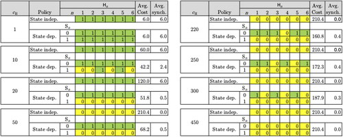
Figure 3. State-independent and state-dependent synchronization policies for different values of the synchronization cost ($c_{\mathrm{H}}$) and their average cost and the number of synchronizations ($c_{\mathrm{B}}=10,$ r = 0.09, p = 0.01, Δ = 10, N = 6, $y_0=1$).

8. Numerical results

We solve the optimization problems given in the preceding section exactly. The solution to these problems yields all the optimal state-independent and state-dependent policies. As benchmarks, the optimal policy under full information and approximate periodic policy are also determined. The optimal periodic state-dependent policy is characterized by the optimal values of the quadruple $({\omega }_1,m_1,{\omega }_0,m_0).$ We analyze the effects of the system parameters on the state-independent and state-dependent policies. We also examine the effects of the system parameters on the average costs and the average number of synchronizations and compare the performance of the optimal state-dependent and state-independent policies with the optimal policy under full information and the approximate periodic policy.

Figure 3 shows the state-independent and state-dependent solutions for different values of the synchronization cost, the average cost, and the average number of synchronizations for each policy. The solutions show that the optimal synchronization policy depends on the balance between the synchronization cost, bias cost, and evaluation period. When the synchronization cost is <50, the state-independent policy synchronizes the digital twin at all evaluation periods. When it is ≥50, the optimal state-independent policy does not synchronize the digital twin at any given time period. On the other hand, when the synchronization cost is <50, the state-dependent policy states that the digital twin should be synchronized at all time periods only when the station is observed to be down (0). When the synchronization cost is ≥20, the optimal state-dependent policy does not allow synchronization when the station is up (1)(1) $${\mathit{S}}_{n+1}=S^{\mathrm{M}}({\mathit{S}}_n,{\mathit{u}}_n)=\{\begin{array}{cc}((y_0,y_1,\dots ,y_k,\dots ,y_n),d_l,{\mathbf{p}}_m)\hfill & ({\mathrm{H}}_n=1,d_n=d_l,{\mathbf{p}}_n={\mathbf{p}}_m)\hfill \\ ((y_0,y_1,\dots ,y_k,\dots ,y_n),d_l,{\mathbf{p}}_n)\hfill & ({\mathrm{H}}_n=1,d_n=d_l,{\mathbf{p}}_n\ne {\mathbf{p}}_m)\hfill \\ ((y_0,y_1,\dots ,y_k,\dots ,y_n),d_n,{\mathbf{p}}_n)\hfill & ({\mathrm{H}}_n=1,d_n>d_l,{\mathbf{p}}_n\ne {\mathbf{p}}_m)\hfill \\ ((y_0,y_1,\dots ,y_k),d_l,{\mathbf{p}}_m)\hfill & ({\mathrm{H}}_n=0,d_n=d_l,{\mathbf{p}}_n={\mathbf{p}}_m)\hfill \end{array}$$(1) . The state-dependent policy also sets a synchronization rule that not only depends on the state of the station, but also the synchronization period. For example, when the synchronization cost is 10, the synchronization policy synchronizes the digital twin when the station is down at any given period or up in the third and fifth periods. Similarly, when the synchronization cost is 250, the state-dependent synchronization policy synchronizes the digital twin when the machine is down in the first, second, third, and fifth periods. When a synchronization policy synchronizes at selected periods in the planning horizon, the selected periods are approximately equally distributed in the planning horizon.

As the synchronization cost increases, the number of synchronizations used by the state-independent and state-dependent policies decreases as expected. While the state-dependent policy determines the states where the digital twin will be synchronized, the average number of synchronizations β depends on the probabilities of visiting these states. As a result, the average number of synchronizations will be lower than the number of states where a synchronization action is required in these states according to the synchronization policy. For example, when $c_{\mathrm{H}}=10,$ the state-dependent policy gives that the digital twin will be synchronized at each period when the machine is found to be down at the time of observation and in addition when the machine is up or down in periods 3 and 5. Although a total of eight synchronization decisions are defined for different state and period pairs, the average number of synchronizations is 2.4 based on the probabilities of observing these states. This is lower than the number of synchronizations used by the state-independent policy that synchronizes at every evaluation period.

The effects of the synchronization cost, average availability of the production system, repair rate, and the number of cycles between the observations are investigated with further experiments given in Appendix D given as an online supplement.

The experiments with varying synchronization cost shows that the average cost obtained using the state-dependent policy is very close to the average cost obtained under the full-information policy. The maximum deviation of the state-dependent policy’s average cost compared with the full-information policy’s average cost is 12% for the cases analyzed. The average number of synchronizations under the state-dependent policy for a given synchronization cost is also very close to the average number of synchronizations under the full-information policy.

The experiments that investigate the effect of the system availability ($u=\frac{r}{p+r}$) show that when the availability is above 60%, the number of parts to be produced during the Δ time periods does not vary much around the expected value. As a result, resource requirement prediction can be done better. This yields a lower number of synchronizations and a lower average cost. When the average availability is lower than 60%, the variability of the number of parts to be produced increases with an increasing u that yields an increase in the total average cost.

For the same average availability, increasing the repair rate increases the probability that the state of the machine is up and running at the time of observations. In this case, observing the state does not improve the synchronization policy, and the state-dependent, state-independent, and full-information policy solutions become closer to each other. Similar to the effect of the repair rate, the number of cycles between the observations affects the policies depending on the likelihood of observing state changes at each observation. As Δ increases, the likelihood of observing that the machine is up and running approaches its steady-state value. Therefore, incorporating the machine’s initial state in the policy does not improve the policies. However, if the observation period allows observing state changes, the state-dependent policy yields a better average cost.

The experiments show that the periodic state-dependent policy yields either exactly the optimal cost or an average cost that is within 2% of the optimal cost. The average percentage difference for 54 cases reported in Appendix D of the online supplement is 0.54%.

9. Conclusions

In this article, the digital twin synchronization problem is introduced and defined formally. The digital twin synchronization problem determines when to synchronize a digital twin and when not to synchronize it at each period depending on the observations to balance the cost of synchronizing a digital twin with the physical system with the benefit of improving the prediction of a performance measure with the synchronization. We define the different variants of the synchronization problem in different contexts. Namely, we discuss the prediction update, model update, and prescription update as different variants of the general synchronization problem.

After giving the general model and formulation of the digital twin synchronization problem, the problem of synchronizing an unreliable production system with its digital twin is formulated. The state-independent, state-dependent, and full-information solutions have been determined by using a stochastic model of the system. Although the problem could be analyzed using discrete-event simulation, the analysis of the stochastic model allows solving the stochastic optimization problem exactly with the scenario approach. This approach allows us to focus on the exact optimal solution without the need to predict the objective function value of the optimization problem by using simulation for each decision and then a simulation-optimization approach.

Our numerical experiments show that the optimal synchronization policy does not synchronize the digital twin at all observation periods. Furthermore, the state-dependent policy incorporating the state of the system, whether the machine is up or down during the observation periods, yields significantly better results than the state-independent solution. The average cost of the state-dependent policy is also close to the average cost that can be obtained with the full information. The effects of the system parameters on the benefits of using a state-dependent policy have been investigated through numerical experiments. We also investigated the optimal control problem in the infinite horizon and suggested an approximate periodic synchronization policy. The comparison of the performance of this policy with the optimal policy shows that the proposed periodic policy is a very good approximation and yields either optimal or near-optimal results. This policy can also be implemented in more complicated systems to determine the synchronization policy.

This research can be extended in different ways. To introduce and analyze the synchronization problem with an analytically tractable special case, we focus on the prediction update problem under the full information case. Accordingly, a scenario approach is used to determine the optimal solution. The general synchronization problem with the decisions on when to update the predictions, the model, and the prescription without the full information is a challenging problem. A sequential decision-making approach, such as reinforcement learning can be used to analyze a case where the effect of the decisions on the overall objective function needs to be estimated from the observed data without requiring an extensive number of simulations.

In the simplified production system example analyzed in this article, the system state is either up or down and fully observable. In a complex manufacturing system, determining when or not to synchronize the digital twin requires developing an indicator based on a subset of the observable states. This is left for future research. In this study, the optimal state-dependent solution for the finite horizon case is determined numerically. A future research challenge is showing the optimal policy structure for the finite and infinite horizon cases.

In conclusion, we show that an optimal digital twin synchronization policy balances the cost of synchronizing a digital twin with the physical system with the benefit of effectively improving the prediction of a performance measure with synchronization. Furthermore, this policy should depend on the system state during the observation periods.

Data availability statement

The data that support the findings of this study are available from the corresponding author upon reasonable request.

Additional information

Funding

Research leading to these results has received funding from Horizon Europe Program under grant agreement no. 101092021 (project Auto-twin).

Notes on contributors

Barış Tan

Barış Tan is a Professor of Operations Management and Industrial Engineering at Koç University, Istanbul, Turkey. His areas of expertise are in design and control of production systems, supply chain management, and stochastic modeling. He received a BS degree in electrical and electronics engineering from Bogazici University, ME in industrial and systems engineering, MSE in manufacturing systems, and PhD in operations research from the University of Florida.

Andrea Matta

Andrea Matta is a Full Professor of Manufacturing and Production Systems at the Department of Mechanical Engineering of Politecnico di Milano (Milan, Italy). He graduated in industrial engineering at Politecnico di Milano where he develops his teaching and research activities since 1998. He was Distinguished Professor at the School of Mechanical Engineering of Shanghai Jiao Tong University from 2014 to 2016. He has been a visiting professor at Ecole Centrale Paris (Paris, France), University of California (Berkeley, USA), and Tongji University (Shanghai, China). He was awarded with the Shanghai One Thousand Talent and Eastern Scholar in 2013. His research area includes analysis, design, and management of manufacturing and health care systems. He is the Editor-In-Chief of Flexible Services and Manufacturing journal.

References

- Ait-Alla, A., Kreutz, M., Rippel, D., Lütjen, M. and Freitag, M. (2019) Simulation-based analysis of the interaction of a physical and a digital twin in a cyber-physical production system. IFAC-PapersOnLine, 52, 1331–1336.
- Ballou, D.P. and Pazer, H.L. (1995) Designing information systems to optimize the accuracy-timeliness tradeoff. Information Systems Research, 6, 51–72.
- Cardin, O. and Castagna, P. (2011) Proactive production activity control by online simulation. International Journal of Simulation and Process Modelling, 6, 177–186.
- Gao, C., Park, H. and Easwaran, A. (2021) An anomaly detection framework for digital twin driven cyber-physical systems, in Proceedings of the ACM/IEEE 12th International Conference on Cyber-Physical Systems, pp. 44–54.
- Hanisch, A., Tolujew, J. and Schulze, T. (2005) Initialization of online simulation models, in Proceedings of the 2005 Winter Simulation Conference, IEEE Press, Piscataway, NJ, pp. 1795–1803.
- Hashash, O., Chaccour, C. and Saad, W. (2022) Edge continual learning for dynamic digital twins over wireless networks. arXiv preprint arXiv:2204.04795.
- Jia, P., Wang, X. and Shen, X. (2021) Digital-twin-enabled intelligent distributed clock synchronization in industrial IoT systems. IEEE Internet of Things Journal, 8, 4548–4559.
- Kuts, V., Modoni, G.E., Otto, T., Sacco, M., Tähemaa, T., Bondarenko, Y. and Wang, R. (2019) Synchronizing physical factory and its digital twin through an IIoT middleware: A case study. Proceedings of the Estonian Academy of Sciences, 68, 364–370.
- Lengerke, C.V., Hefele, A., Cabrera, J.A. and Fitzek, F.H.P. (2022) Stopping the data flood: Post-Shannon traffic reduction in digital-twins applications, in NOMS 2022-2022 IEEE/IFIP Network Operations and Management Symposium, IEEE Press, Piscataway, NJ, pp. 1–5.
- Lugaresi, G. and Matta, A. (2018) Real-time simulation in manufacturing systems: Challenges and research directions, in 2018 Winter Simulation Conference (WSC), IEEE Press, Piscataway, NJ, pp. 3319–3330.
- Manothiang, M. and Nuratch, S. (2021) IoT device and virtual representation application design and implementation for physical world and virtual world real-time synchronization, in 2021 International Conference on Electrical, Computer and Energy Technologies (ICECET), pp. 1–6.
- Müller, M.S., Jazdi, N. and Weyrich, M. (2022) Self-improving models for the intelligent digital twin: Towards closing the reality-to-simulation gap. IFAC-PapersOnLine, 55, 126–131.
- Modoni, G.E., Caldarola, E.G., Sacco, M. and Terkaj, W. (2019) Synchronizing physical and digital factory: Benefits and technical challenges. Procedia CIRP, 79, 472–477.
- Moore, J.C. and Whinston, A.B. (1986) A model of decision-making with sequential information-acquisition (part 1). Decision Support Systems, 2, 285–307.
- Negri, E., Pandhare, V., Cattaneo, L., Singh, J., Macchi, M. and Lee, J. (2021) Field-synchronized digital twin framework for production scheduling with uncertainty. Journal of Intelligent Manufacturing, 32, 1207–1228.
- Powell, W.B. (2021) From reinforcement learning to optimal control: A unified framework for sequential decisions, in Handbook of Reinforcement Learning and Control, Springer International Publishing, Cham, Switzerland, pp. 29–74.
- Qin, Y., Ma, M., Shen, L., Wang, H. and Han, J. (2022) Virtual and real bidirectional driving system for the synchronization of manipulations in robotic joint surgeries. Machines, 10, 530.
- Sargent, R.G. (2013) Verification and validation of simulation models. Journal of Simulation, 7, 12–24.
- Tan, B. (1999) Variance of the output as a function of time: Production line dynamics. European Journal of Operational Research, 117, 470–484.
- Tan, B. and Matta, A. (2022) Optimizing digital twin synchronization in finite horizon, in Proceedings of the 2022 Winter Simulation Conference, IEEE Press, Piscataway, NJ, pp. 2924–2935.
- Tao, F., Qi, Q., Wang, L. and Nee, A. (2019) Digital twins and cyber–physical systems toward smart manufacturing and industry 4.0: Correlation and comparison. Engineering, 5, 653–661.
- Zipper, H. (2021) Real-time-capable synchronization of digital twins. IFAC-PapersOnLine, 54, 147–152.
- Zipper, H. and Diedrich, C. (2019) Synchronization of industrial plant and digital twin, in 2019 24th IEEE International Conference on Emerging Technologies and Factory Automation (ETFA), IEEE Press, Piscataway, NJ, pp. 1678–1681.