Analyzing illegal psychostimulant trafficking networks using noisy and sparse data

Abstract

This article applies analytical approaches to map illegal psychostimulant (cocaine and methamphetamine) trafficking networks in the US using purity-adjusted price data from the System to Retrieve Information from Drug Evidence. We use two assumptions to build the network: (i) the purity-adjusted price is lower at the origin than at the destination and (ii) price perturbations are transmitted from origin to destination. We then adopt a two-step analytical approach: we formulate the data aggregation problem as an optimization problem, then construct an inferred network of connected states and examine its properties.

We find, first, that the inferred cocaine network created from the optimally aggregated dataset explains 46% of the anecdotal evidence, compared with 28.4% for an over-aggregated and 14.5% for an under-aggregated dataset. Second, our network reveals a number of phenomena, some aligning with what is known and some previously unobserved. To demonstrate the applicability of our method, we compare our cocaine data analysis results with parallel analysis of methamphetamine data. These results likewise align with prior knowledge, but also present new insights. Our findings show that an optimally aggregated dataset can provide a more accurate picture of an illicit drug network than can suboptimally aggregated data.

Keywords:

• Illicit supply chains
• cocaine
• methamphetamine
• data aggregation
• cocaine trafficking
• network analysis
• USA

1. Introduction

The global economic network grows more complex every day. Increased connectivity presents growing opportunities for people and businesses engaged in licit activities worldwide, but it also fosters illicit trafficking networks. Such illicit trafficking creates resource flows that are external to the formal economy and enormous in scale: the United Nations Office on Drugs and Crime (UNODC) estimates that transnational criminal organizations reap profits of approximately $870 billion USD per annum (UNODC, 2018). This shadow economy not only results in loss of revenue for governments and industries globally, but also more importantly, it threatens public security, health, and safety while enriching Transnational Criminal Networks (TCNs) that have a vested interest in undermining the rule of law.

To effectively mitigate the global threat of illicit supply chains, public and private sector decision makers need a clear and analytically-based understanding of the ecosystem of illicit trafficking networks. Our work contributes to that goal, focusing on appropriate analytical approaches to produce optimally aggregated data to map the cocaine supply chain in the US. Our focus on cocaine is well justified. As the 2019 National Drug Threat Assessment shows, cocaine trafficking is re-emerging as a major problem. In recent years, levels of cocaine availability, cocaine seizures, and deaths from cocaine overdose were high enough to be of special concern to the US government. Approximately 2,3000,000 people nationwide use cocaine at least once per week, and these users constitute the majority of consumers in a $24 billion illicit market (Midgette et al., 2019). Cocaine-related deaths in North America rose from 5000 in 2013 to 14,000 in 2017 and remained at that level through 2021, reflecting an increase in harmful cocaine use, due in part to the introduction of fentanyl into the cocaine supply.

In order to map the flows of the US cocaine supply chain, we gained access to the System to Retrieve Information from Drug Evidence (STRIDE) dataset, which contains nearly 1,800,000 event observations (1982–2014) for US-wide domestic counternarcotics operations. Using this seizure and undercover purchase data, we aim to infer the underlying network structure based on two principles. First, for two connected nodes in the network, one of which (the origin) is sending cocaine to the other (the destination), the purity-adjusted price (henceforth “price”) of the drug will be lower at the origin than at the destination, because the risks (both direct and indirect) of transportation, combined with cumulative transportation, labor, and transaction costs, are assumed to increase price. Therefore, the price gradient between two nodes in a dyad provides information on the direction of flow. Second, for two nodes in the network, local perturbations in price (resulting, e.g., from the impact of local law enforcement specific to the origin node or from other supply chain disruptions) will be transmitted from the origin to the destination. As a result, the price co-movement between these two nodes will be higher than the “background” co-movement in price seen in the network as a whole (due to, e.g., seasonality, law enforcement activities in the source country). In other words, if the measure of price co-movement for two nodes exceeds a certain baseline threshold, then the two nodes can be inferred to be connected.

One challenge presented by the STRIDE data arises from the fact that it has both a geospatial dimension and a time dimension. Each record represents an event, for example, a single undercover purchase, and the density of the data fluctuates across both time and space. A key challenge, therefore, is to optimally aggregate the data over time to compute price gradients and co-movement between pairs of locations. Prior research has typically aggregated data into monthly, quarterly or yearly observations (NDIC, 2004; 2011), but we argue that this approach may not maximize the information benefit of the data, and an ad-hoc approach may result in too short or too long an aggregation period. We therefore propose an optimization approach to determine the optimal aggregation.

In this optimization approach, our goal is to establish whether two nodes (e.g., US states) are connected in the supply chain network. If the time period over which the data are aggregated is too long, then the resulting dataset will have a smaller number of periods, signals may be lost due to over-aggregation, and statistical power may be insufficient due to too few observations. Similarly, if the period is too short, the dataset may have insufficient numbers of periods in which both nodes (e.g., states) have sufficient time-matched information to support the comparison. The aim of this study is therefore to explore ways in which disaggregated data can be aggregated to achieve two objectives. The first objective is to obtain a dataset containing time-matched data for pairs of nodes, thereby facilitating analyses of price co-movement that require time-matched data. The second objective is to maximize the number of usable observations, and therefore the information entering the analysis, subject to the first objective.

Therefore, although our overall goal is to map the illicit supply chain of cocaine, the proposed methodology has broader impact. Empirical social scientific research often involves the analysis of time-tagged panel (i.e., cross-section/time series) data. The time dimension of these data is usually measured in regular intervals (e.g., months, quarters, or years). A common problem with such data is their unbalanced nature, or the presence of “holes.” In other words, the time periods for which data are available for a particular individual or location may not match the time periods for which data are available for other individuals or locations. This mismatch renders the use of analytic methods that rely on time-matched data, such as measures of co-movement (including correlations) impossible. One solution to this problem of mismatched data is aggregation. If time periods can be selected such that observations across individuals or locations are contained within those time periods, then, for each pair of individuals or locations, balanced aggregated panel data can be created. The optimal aggregation approach is a promising novel idea that can maximize the utility of observational data. A second remedy for a dataset with holes is imputation, which assumes smoothness in the data-generation process. Consequently, imputation can introduce smoothness into the data; this smoothness can artificially dampen or inflate measures of co-movement, thereby providing biased measures. Therefore, imputation is not well suited for our purposes, as our goal is to understand and utilize the fluctuating nature of prices, and it is these fluctuations that drive our study of connectivity between nodes.

The remainder of this article is organized as follows. We first briefly review the related literature in Section 2 before introducing the STRIDE data in more detail in Section 3. Next, we introduce the optimal data aggregation approach in Section 4 and apply it to the STRIDE cocaine data. In Section 5 we build the cocaine network based on the optimal aggregation, comparing the results to anecdotal evidence. Next, we demonstrate a second application of the two-step methodology to methamphetamine data in Section 6 and compare the obtained methamphetamine network with the cocaine network. We conclude with implications and directions for future research in Section 7.

2. Background

2.1. Using prices and other variables to identify networks

The identification of trafficking routes for illicit drugs is of great interest to the law enforcement and drug policy research communities (Giommoni et al., 2017). For law enforcement, identifying routes and important nodes can inform the allocation of resources to optimally disrupt networks of drug flows (Giommoni et al., 2021). For the drug policy research community, knowing the structure of the network can enable well-contextualized studies of the impacts of illicit drugs, drug flows, and drug markets on phenomena ranging from crime to health (Boivin, 2014). Unlike transportation routes for legal goods, however, information about flow networks for illicit drugs is difficult to come by, and even when it is available, it is often incomplete and inaccurate. This scarcity of information has motivated a growing literature on ways to use existing data on drugs and drug markets to infer the structure of the drug flow network.

The most widely available types of data on illicit drugs include seizures, prices, and purity. Seizure data are reported in a number of different locations, including the US and various European countries, via a variety of media including digital datasets and reports by government and multilateral organizations such as the United Nations and the European Union (UNODC 2021a).

These seizure datasets usually contain information about quantities and types of drugs seized along with spatial and temporal information relating to the seizure or seizures. As the name suggests, these data are usually obtained as a result of drug interdiction operations. Price data are also reported by the US and a number of European countries and are obtained through undercover drug purchases or as part of interactions between law enforcement professionals or informants and drug sellers or buyers (NDIC, 2004; 2011; USDOJ, 2014; UNODC, 2021b). Purity data are derived from seized or purchased samples and often accompany the data on prices and seizures (USDOJ, 2014; UNODC, 2021).

In recent years, economists and drug policy researchers have paid increasing attention to drug prices as a source of valuable information about trafficking. Indeed, as Hayek argued over half a century ago (Hayek, 1945), prices are a rich source of information and help authorities efficiently allocate scarce resources for optimal use. The basic premise of prices as a source of information about illicit drug flows is supported by a variety of prior studies. In one early one, (Farrell et al., 1996) observed that wholesale prices of drugs in Europe tended to be lowest in the locations through which the drugs were entering the continent. As drugs travel from producers to end users, they often change hands in a series of transactions, each of which pushes the price of the drug up because of the incremental costs of “personnel, transportation, and corruption” (Reuter, 1988). The incremental risk involved in successive transactions also contributes to these increases (Reuter and Kleiman, 1986; Caulkins and Reuter, 1998). Unsurprisingly, therefore, prices of illicit drugs increase with the distance from their source (Caulkins and Bond, 2012).

Drawing on this basic premise, Chandra et al. (2011) used price data to infer the network of transnational cocaine flows across 17 western European countries using data from UNDOC’s World Drug Reports. Two basic principles were used to infer flows between any given pair of countries. First, the direction of a flow was inferred on the basis of the price gradient between the two countries: flowing from the country with the lower price to the country with the higher one. Second, in order to infer the presence of a flow between a pair of countries, the correlation in the prices of cocaine in the two countries was required to exceed a specified threshold. The logic for this requirement was that if a country was receiving the drug from another country in any significant measure, then any shocks to the price in the originating country would be transmitted to and would therefore be visible in the price in the destination country. Using this method, researchers have leveraged price data to estimate the following flow networks: cocaine across Europe (Chandra et al., 2011) and heroin across Europe (Chandra and Barkell, 2013), powdered cocaine across the US (Chandra et al., 2014), and cocaine hydrochloride across Colombia (Benítez et al., 2019).

The STRIDE data, on which this article builds, have been used to evaluate illegal drug market size and structure and to estimate the impact of drug prices and drug use on public health and safety. Specifically, they have been used to estimate the size and value of domestic US markets for cocaine, heroin, and methamphetamine (Kilmer et al., 2014; Midgette et al., 2019), to describe geographic variation (Caulkins, 1995), to estimate volume discounts and risk premia (Caulkins and Padman, 1993; Caulkins and Reuter, 1998; Miron, 2003), and to infer supply decisions in the cocaine market (Caulkins, 1997). Price estimates from STRIDE have also been used to measure demand responses to supply interdiction actions (Grossman and Chaloupka, 1998; Saffer and Chaloupka, 1999; DeSimone and Farrelly, 2003) and harms associated with drug use (Dave, 2006; Dobkin and Nicosia, 2009; Cunningham and Finlay, 2016). To date, however, STRIDE data have not been used to identify cocaine flows across the US. This is one of the goals of this article.

Although the use of price gradients to infer the direction of flows and of price co-movements to infer connectivity between nodes in the flow network may be intuitively obvious, it is important to acknowledge the limitations of using gradients and co-movements in price between nodes as indicators of flows. Prices may vary for reasons other than transmission. For example, the increased intensity of law enforcement in a particular node at a particular time may briefly drive up the price of cocaine in that location, causing its price to vary out of step with prices in nodes that precede it in the supply chain. Seasonal fluctuations may also drive variations in price, though these are more likely to be systematically transmitted across the network, especially if that seasonality is associated with the cultivation of the coca plant, which grows in South America, thereby causing aggregate (i.e., network-wide) rather than idiosyncratic (i.e., node-specific) fluctuations in prices at nodes located in the US. Notably, since our analysis is restricted to data for non-retail transactions, to the extent that nodes are affected by such idiosyncratic factors, they may still transmit these shocks to downstream nodes, thereby preserving the tendency for gradients and co-movements in price to capture the basic structure of the network, however imprecisely.

Finally, our article builds on and extends the literature of data aggregation. The study of data aggregation is common and has a long tradition (Orcutt et al., 1968) in multiple domains. In the social sciences, the impact of data aggregation has been studied in different contexts. For example, a recent paper studied the impact of data aggregation on policy decisions and found that aggregation impacts both the level of investment and the technology chosen (Khavari et al., 2021). Similarly, a separate study highlighted that data aggregation can influence subsequent inferences (Shellman, 2004). In summary, the literature has acknowledged the importance and the potential impact of data aggregation. However, formalizing the aggregation problem as an optimization problem to maximize learning has, to the best of our knowledge, not yet been suggested. In this study we formulate the aggregation problem as an optimization problem with the objective of maximizing the possible learning from a dataset.

3. Data

The Drug Enforcement Administration (DEA) has maintained STRIDE as a central repository for transaction-level drug enforcement data from federal, state, and local law enforcement agencies in the US beginning in the late-1970s. STRIDE observations describe purchases and seizures, timing and location information, the total amount paid when the transaction involved a purchase, illicit substances involved, and measures of quantity and purity. STRIDE is the only source of data for US-wide domestic counternarcotics operations including undercover purchases (14% of observations). In this article, we focus on the cocaine transactions that include price information (n = 84,953 out of a total of 258,672 cocaine transactions). Each event record includes the weight of the drug, location (at the state level), year, month, purity of sample, and price paid.

Prior work demonstrates that analyses of STRIDE data should be conducted and interpreted with caution (Arkes et al., 2008) as they are generated by non-random drug enforcement actions and exhibit improbably high within-jurisdiction price variation that renders them inappropriate for policy analyses (Horowitz, 2001; Manski et al., 2001). In the present analysis, we do not attempt to evaluate within-city variation or the impact of policy. Rather, we examine the price gradients across states. We acknowledge that the point estimates of mean or median prices per pure gram we evaluate are measured with error, but that between-state error in prices is random.

This analysis focuses on variation in the price per pure gram of cocaine. Price variation is associated with the underlying purity of the purchased drug: since most street-level cocaine transactions involve products that are not pure cocaine, but rather a mixture whose exact composition is not known to the buyer, drugs that are purer command a price premium (Caulkins, 2007). Drugs involved in larger wholesale transactions are typically purer (Arkes et al., 2008). We thus divide nominal price paid by recorded purity, bound by zero and one, to generate a purity-adjusted price per pure gram. For our analysis, we filter the sample to undercover purchases involving quantities of at least 5 grams and no more than 1 kilogram, thus focusing on observations that are more representative of the wholesale and trafficking market than more variable street-level purchases. Further excluding observations with missing potency information leaves 59,676 records to be analyzed. Summary statistics are shown in Table 1, and Figure 1 highlight the relationship between weight and price per pure gram of cocaine. We note the very large variation in price per pure gram, especially for smaller purchases.

Figure 1. An overview of the study sample ranging from 1 g to 1 kg. Excluded from the figure are 74 observations for which the price per pure gram exceeded $1000.

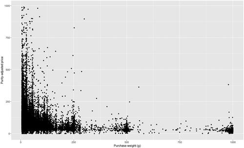
Table 1. Sample means for purity, weight, and price per transaction, gram and pure gram.

Variable	All cocaine transactions with price (n= 84,9539)	The study sample (n = 59,676)
Potency (%)	61.74	61.95
Weight (g)	46.3	54.5
Price (per transaction)	1453	1830
Price per gram	460.8	44.6
Purity-adjusted price	175.6	87.6

Following earlier work, the variable we used in our analysis is the purity-adjusted price (Kilmer et al., 2014; Midgette et al., 2019). We choose purity-adjusted price because the appropriate metric to quantify the amount of cocaine being sold is not the physical weight of the material transacted, but rather the amount of cocaine contained in that material. Therefore, a 100-gram sample of 50% pure cocaine should have the same price as a 50-gram sample of 100% pure cocaine. We compute the purity-adjusted price as the amount paid for a sample divided by the product of the weight of the sample and its purity, or $$P_{\mathit{adj}}=\frac{P}{W·\Psi }$$ where P_adj is the purity-adjusted price per unit weight of a sample of cocaine, P is the price paid for the sample, W is the weight of that sample (in grams), and $\Psi$ is the percentage purity of the sample.

4. Optimization approach to data aggregation

We now introduce our data aggregation optimization approach. Our goal is to find the optimal aggregation in order to maximize the ability to support network generation. More specifically, our goal is to determine the optimal length of the aggregation period, ${\tau }^{*},$ to maximize the potential learning from the data. In the context of mapping the cocaine supply network, maximizing learning corresponds to accurately measuring state-level correlations and price levels.

Let I be the set of states and let t be a month (which reflects the most granular level of the STRIDE data that are publicly available). Given the complexities of the STRIDE data, assume a minimum number κ that is required to estimate the price in a given state in a given aggregation period. Our goal is then to maximize the number of state-state periods with at least κ observations in both states.

Let n_it be the number of records in state i in time period t. Let $x_{ii\prime l}$ be a binary indicator that is 1 if in period l there are at least κ observations in states i and $i\prime ,$ and 0 otherwise, where l is an index of an aggregation period of length τ. Further, let d_il be the number of observations in aggregation period l in state i. In order to capture the start and end of each period, we define:

• t_s as the first period of observations (accounting for the lack of data often observed in the first few periods as data collection is scaling up), and

• $p_l^s$ as the start time of period l.

Finally, let T represent the maximum number of aggregation periods (which is bounded from above by the number of observation periods). We can then express the data aggregation as the following optimization problem where τ and t_s are the decision variables: (1a) $$\mathrm{}{\max }_{}\mathrm{\hspace{1em}}\mathrm{\hspace{1em}}\frac{1}{2}\sum _i\sum _{\prime i}\sum _l{x}_{ii\prime l}$$(1a) (1b) $$\text{subject to\hspace{1em}}{p}_1^s=t_s$$(1b) (1c) $$p_{l+1}^s=p_l^s+\tau \forall l=1,\dots ,T$$(1c) (1d) $$d_{il}=\sum _{t=p_l^s}^{p_l^s+\tau -1}{n}_{it}\mathrm{\hspace{1em}}\mathrm{\hspace{1em}}\forall i,l=1,\dots ,T-1$$(1d) (1e) $$x_{ii\prime l}\le d_{il}/\kappa \forall l,i,$$(1e) (1f) $$x_{ii\prime l}\le d_{i\prime l}/\kappa \forall l,i\prime$$(1f) (1g) $$\tau ,t_s\ge 0$$(1g) (1h) $$x_{ii\prime l}\in \{0,1\}.$$(1h)

Given that the size of the cocaine dataset does not present a computational challenge, we solve the above model with exhaustive search, iterating over integer values of τ. More specifically, for each integer value of τ, we iterate through t_s, each time aggregating the data based on τ and t_s parameters. For larger data, one would like to optimize τ using commercial solvers.We therefore provide in the online supplement an expanded formulation of the model as a linear optimization model (with big M constraints).

Consider the entire cocaine data. Figure 2(a) highlights the optimal value as a function of κ. The figure highlights the dependency of ${\tau }^{*}$ on κ. When we set κ equal to 25, we note that ${\tau }^{*}$ is eight, highlighting that ad-hoc aggregation into 3-, 6-, or 12-month intervals, which is typical (NDIC, 2004; 2011), may indeed be suboptimal.

Figure 2. The objective value as a function of τ. On the left (a) the objective function is the number of state-state periods with at least κ observations in each state; on the right (b) we have the number of state-state pairs with at least κ = 25 observations in at least γ aggregated periods.

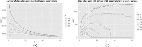
However, we note that a state-state pair with a low number of aggregated periods that meet the requirement may not add to our ability to estimate the underlying network. For example, if Alabama and Georgia have enough data in a single aggregated period, it is not enough to estimate the correlation of prices between the two states. For our use case, we therefore need to update the formulation to only consider state pairs that have at least γ periods in the objective function. This requires a straightforward expansion of the previous formulation: (2a) $$\mathrm{}{\max }_{}\mathrm{\hspace{1em}}\frac{1}{2}\sum _i\sum _{\prime i}{c}_{ii\prime }$$(2a) (2b) $$\text{subject to }{p}_1^s=t_s$$(2b) (2c) $$p_{l+1}^s=p_l^s+\tau \forall l=1,\dots ,T-1$$(2c) (2d) $$d_{il}=\sum _{t=p_l^s}^{p_l^s+\tau -1}{n}_{it}\mathrm{\hspace{1em}}\mathrm{\hspace{1em}}\forall i,l=1,\dots ,T-1$$(2d) (2e) $$x_{ii\prime l}\le d_{il}/\kappa \forall l,i,$$(2e) (2f) $$x_{ii\prime l}\le d_{i\prime l}/\kappa \forall l,i\prime$$(2f) (2g) $$c_{ii\prime }\le \frac{1}{\gamma }\sum _{l=1}^T{x}_{ii\prime l}\forall i,i\prime$$(2g) (2h) $$\tau ,t_s\ge 0$$(2h) (2i) $$x_{ii\prime l},c_{ii\prime }\in \{0,1\},$$(2i) where $c_{ii\prime }$ is a binary indicator equal to one if state i and state $i\prime$ have at least κ observations each in at least γ periods. We note from Figure 2(b) that the optimal τ is quite sensitive to the value of γ. When γ is small, τ is large, reflecting a benefit in the count from including lower data density pairs. When γ is larger, ${\tau }^{*}$ ranges from 5 (for γ = 30) to 23 (for γ = 10). It should also be noted that the optimal ${\tau }^{*}$ values are sensitive to the value of κ; however, the magnitude of the impact on the value of ${\tau }^{*}$ depends on the characteristics of the underlying data.

Our data aggregation approach can potentially be expanded to allow τ to adapt to time-varying data density and to additional aggregation across the geographical dimension (e.g., combining neighboring geographic units in our case states). More generally, if the goal is to find an optimal aggregation to maximize learning from the data, we can define an objective function $f(\tau ),$ which links the number of records in a period at a location to the overall goals of the statistical project. As before, the goal is to determine the optimal length of the aggregation period ${\tau }^{*}.$ At a high level, we then express the optimization problem as: (3) $$\begin{array}{ccc}\underset{{}_{t_s,\tau }}{\max }& f(t_s,\tau )& \\ \mathrm{s}.\mathrm{t}.& p_1^s=t_s& \\ & p_{l+1}^s=p_l^s+\tau & \forall l=1,\dots ,T-1.\end{array}$$(3)

5. Mapping the supply network

Using the optimally aggregated data, we constructed a network representing the cocaine supply chain. We ran the optimization approach described above and found ${\tau }^{*}$ to be 20, requiring κ of 15.

For each state and time period, as described above, the aim was to obtain a measure of the purity-adjusted price of cocaine that would allow for the computation of price gradients between pairs of states to infer the direction of cocaine flows and of price correlation. This in turn would allow us to infer whether or not a flow of cocaine occurs between the two states. In order to do this, we computed a number of measures of purity-adjusted price, including the mean purity-adjusted price of cocaine, the median purity-adjusted price of cocaine, and four sets of prices that were generated through regression modeling, using both ordinary least squares and robust regression on purity-adjusted price and the log of purity-adjusted price. For comparison, we also computed the mean price and the median price of cocaine, unadjusted for purity.

After examining the distributions of these various alternatives, we picked the median purity-adjusted price of cocaine because this variable is not heavily influenced by outliers or by the variation in purity across observations. Our choice was also motivated by evidence that per unit prices of cocaine are influenced by purity. Also supporting this choice, we found in our empirical experiments that the concordance rate (described below) was typically as high as that obtained using the more sophisticated approaches to establishing the price in a state in a given time period.

5.1. Ground truth

The anecdotal data were extracted from the map in Figure 3. The basic pattern in the map shows that cocaine enters through points in the south of the country and flows in a north and northeasterly direction. This, of course, corresponds with the South American source of cocaine, extracted from the coca plant, which thrives in the Andean countries of Colombia, Peru, and Bolivia. Key entry states include California and Texas and, possibly, Arizona and New Mexico, all of which share borders with Mexico, where multiple powerful drug trafficking organizations operate.

Figure 3. Routes for cocaine flows across the US; Source: (USDOJ, 2011).

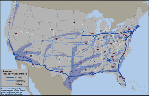
The anecdotal dataset listed all pairs of adjacent states through which a cocaine trafficking route went along with the direction in which the cocaine was flowing. Next, we augmented this initial (first-order) anecdotal dataset to include state-state pairs i, j if there existed a state k such that i was connected to k and k was connected to j, producing what we call pairs of the second degree. Third, we added state-state pairs that, based on the anecdotal evidence, could be connected through at most two other states, calling them pairs of the third degree. We repeated this process until a subsequent iteration of the process yielded a network with no new flows (i.e., the network converged with or was identical to the preceding iteration). In the case of the cocaine map in Figure 3, the network of anecdotal flows converged on the eighth iteration.

Note that in Figure 3, a number of states are not linked to any other states. These include Alaska, Hawai’i, Idaho, Maine, Montana, New Hampshire, and Vermont. This means that the maximum number of possible state-state pairs for which flows based on the map can be recorded in the anecdotal dataset is $\left(\begin{array}{c}43\\ 2\end{array}\right)$ = 903. This is substantially lower than the total number of possible state-state pairs (i.e., $\left(\begin{array}{c}50\\ 2\end{array}\right)$ = 1225) in the inferred dataset, where the price data comes from all US states. Therefore, any measure of fit between the anecdotal and inferred networks is unlikely to be high.

5.2. Calibration

In this section, we report on the overlap between the anecdotal evidence and the inferred network before discussing the complete network. As explained above, although our network analysis includes all possible state-state pairs, the anecdotal evidence was initially summarized on the adjacent state level. We found that as we included higher-order connections, the percentage of overlap between the anecdotal network and the inferred network increased. This is highlighted in Figure 4(a), which shows the percentage of anecdotal links contained in the inferred network when the correlation threshold is calibrated to maximize this overlap between the two datasets (the correlation threshold varies from 0.58 for the lower degree anecdotal networks to 0.52 for the higher-order networks). A drawback of using the percentage of anecdotal links contained in the inferred dataset is that there is no penalty for including larger numbers of possibly spurious inferred links. This will tend to push the calibration threshold value down, thereby introducing noise in the form of spurious inferred links, into the inferred flow network.

Figure 4. Network Calibration: (a) The percentage of anecdotal links contained in the inferred network when the correlation threshold is set to maximize the concordance between the two datasets and (b) the concordance rate, when the correlation threshold is set to maximize the concordance between the the anecdotal links and the inferred links.

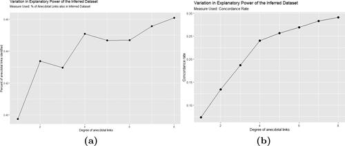
A remedy for this bias is to create a measure that incorporates a penalty for the unnecessary inclusion of inferred links that have no explanatory power. A natural measure of fit that satisfies this property is the concordance rate, defined as the size of the intersection of the anecdotal and inferred datasets (i.e., the number of pairs of states appearing in both datasets) divided by the size of the union of the two datasets (i.e., the total number of unique state-state pairs appearing in one or both of the datasets), (4) $$C=\frac{|A\cap I|}{|A\cup I|},$$(4) where A is the anecdotal dataset, I is the inferred dataset, and C is the concordance rate. Note that inferred pairs that are not in the anecdotal dataset will increase the size of the denominator without increasing the value of the numerator, thereby creating a penalty for adding inferred links that have no explanatory power in relation to the anecdotal dataset.

Figure 4(b) shows the concordance rate between the anecdotal and inferred links for each iteration in the anecdotal dataset at the concordance-maximizing value of the correlation threshold for each iteration. As in the case of the earlier measure of fit (see Figure 4(a)), as we include higher-order connections the concordance rate increases. We note that the corresponding correlation thresholds for the first- and second-order anecdotal datasets are much higher (0.8 and 0.7) than they are for the higher-order datasets (which vary between 0.52 and 0.57), with a value of 0.57 for the concordance-maximizing eighth iteration. This value is slightly higher than the concordance-maximizing correlation threshold of 0.52 obtained for the eighth iteration using the earlier measure of fit, reflecting a more conservative link inclusion.

5.3. The resulting network

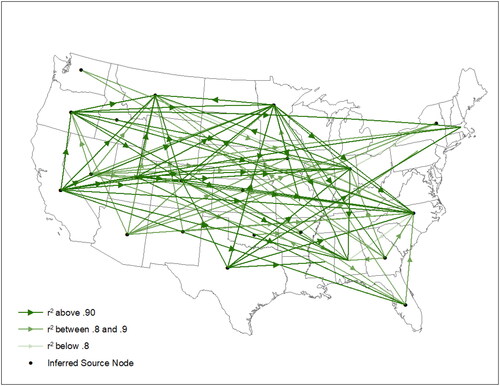
Figure 5 is a map of the inferred flows using the optimally aggregated data and the concordance-maximizing threshold correlation. The network contains 46% of the anecdotal links and the overall concordance rate is 29%.

Figure 5. Inferred cocaine flows based on the analysis of concordance rates. Flows between observed state-state pairs from the optimal ${\tau }^{*}$ specification are visualized such that arrows representing $r^2>.9$ are opaque and lower correlation relationships become progressively more transparent.

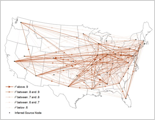
A number of interesting phenomena emerge from the map. First, there is a general tendency for the flows to move in a northerly or northeasterly direction. This is illustrated by, for example, the arrows emanating from California, Arizona, and Texas, which are important points of origin for cocaine moving northward to the interior of the country. This pattern matches the map in Figure 3 and reflects the fact that these three states border Mexico, from which cocaine enters the US. In the Midwest, Illinois appears to be a hub, receiving cocaine from a number of the entry states and sending it to the neighboring states of Wisconsin to the north, Missouri to the south, and Indiana to the east. Indiana, for its part, also appears to be a local distribution hub. On the eastern seaboard, Maryland and New Jersey appear to be hubs for the distribution of cocaine to other states in the region, although Virginia appears to be a destination for flows coming from Texas, Illinois, and Indiana. A number of states appear to have a preponderance of weak links, i.e., links characterized by low price correlations, suggesting weaker linkages with other states. These include New Mexico, New York, Michigan, North Carolina, and South Carolina. In addition, the five states on the map in Figure 3 through which cocaine trafficking routes do not pass, namely Idaho, Montana, New Hampshire, Vermont, and Maine, also appear to not be integrated into the cocaine network in Figure 5. Although data for those states are present in the optimally aggregated dataset, they are insufficient in number to generate price-based correlations with other states and thus are absent from the map. It is possible that the scarcity of underlying cocaine price data in these states may reflect a comparative lack of trafficking activity.

5.3.1. Selected properties of the cocaine network

The data displayed in Figure 5 also lend themselves to network analytic methods. Although not the central subject of this article, it is possible to systematically summarize various network- and node-level phenomena to shed light on the network (Chandra and Joba, 2015). Properties of particular interest include in- and out-degrees of specific states and measures of density, which may illuminate nodes that are particularly good targets for disruption. Methods such as core-periphery analysis and other node-grouping techniques may provide information about the underlying organizational structures operating in different parts of the US, providing a basis for comparison with anecdotal information on the different markets in which different cartels operate. To explore these properties of the network, we used the UCINET software (Borgatti, Everett, and Freeman, 2002).

Table 2 summarizes selected aggregate properties of the cocaine flow network. The measure of density (19%), which is the number of edges in the network as a percentage of the total number of possible edges, demonstrates that the network is sparse. The triad census, also described in the table, is a census of the six different types of triads (i.e., combinations of three nodes) that can occur in a directed acyclic (the use of price gradients to infer direction of flow rules out the possibility of cycles) network. The six types of triads that can occur include the empty triad (no edges), a triad with one edge, three types of triads with two edges (an out-star, with two edges emerging from a single node to the other two nodes; an in-star, with two edges converging from two nodes to a single node; and a directed line, in which an edge emerges from one node and ends at a second node from which an edge to the third node emerges), and a triad with three edges that combines the out-star with the in-star. A figure showing these triad types is provided in the online supplement. Notable properties of the cocaine network, which will be revisited in Section 6.1, include (i) 68% of the triads are non-empty and (ii) 57% of the triads with two or more edges are out-star to in-star (i.e., three-edge) triads.

Table 2. Aggregate properties of the US cocaine flow network. * For details on triad census, refer to the online supplement.

Analysis	Property	Measure
Density	Density	19%
Triad census*	Empty subgraph (% of all triads)	6256 (32%)
	Non-empty triad	13,334 (68%)
	Single edge (% non-empty triads)	7509 (56%)
	Out-star (% triads with 2+ edges)	911 (16%)
	In-star (% triads with 2+ edges)	643 (11%)
	Directed line (% triads with 2+ edges)	948 (16%)
	Out-star to in-star (% triads with 2+ edges)	3326 (57%)
Core–periphery	Core members	21
	Periphery members	29
	Core density	0.49
	Periphery density	0.02
	Fitness measure	0.57

The core-periphery structure (Borgatti and Everett, 1999) of a network can also provide insights into its functioning. Core-periphery analysis is a means of partitioning the nodes in the network into two groups: a core group (or sub-graph) in which members are closely and densely linked with one another and a periphery group, in which members are sparsely linked with each other. In the case of the cocaine network, the core consists of 21 states and the periphery consists of 29 states. Of the 21 core states in the cocaine network (see the online supplement for a complete list), 16 are located east of the Mississippi at some distance from the western and southwestern states that are considered to be major entry points for cocaine into the US.

5.4. Sensitivity analyses

To highlight the importance of optimal data aggregation, we ran two additional scenarios using over-aggregated and under-aggregated data. Specifically, we aggregated the data into quarterly (3-month) time periods on one hand and 5-year (60-month) time intervals on the other. We acknowledge that the value of estimating any statistics associated with drug trafficking in 5-year intervals has little practical utility (e.g., synthetic opioid deaths increased tenfold over 2013-2018); however, the intent of this analysis is to contrast the optimal aggregated solution with the networks based on suboptimal values of τ.

Running the network analysis for the under- and over-aggregated data, we observed that the percentage of anecdotal links in the inferred datasets are 14.5% and 28.4%, respectively, (compared with 46% for the base case) and the concordance rates are 12.6% and 19.5%, respectively, (compared with 29.1% for the base case). Figure 6 summarizes the resulting networks.

Figure 6. The resulting networks for under-aggregation (top) and over-aggregation (bottom). Flows between observed state pairs are visualized such that arrows representing $r^2>.9$ are opaque and lower correlation relationships become progressively more transparent.

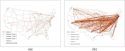
What Figure 6(a) clearly demonstrates is that when the data are under-aggregated, the inherent noise in the data appears to outweigh the correlations; the links are typically weaker, and we note that the strongest link in the network appears to be a spurious link between New York and Minnesota. We also note that in stark contrast to the base case network, Arizona is not connected at all. From Figure 6(b) we note that numerous links have very strong correlation, reflective of the over-aggregation and reducing the correlation analysis to nationwide price trends. Neither case is useful for extracting meaningful insights.

6. Inferred methamphetamine flows

As a second example we repeat our two-step process, this time building the spatial supply chain network for methamphetamine. Methamphetamine (also known as meth, crank or crystal meth) was first synthesized in the late-1800s and was initially used as a medical treatment. During World War II it was used to keep troops awake, and its use increased after the war. After being outlawed in the US in 1970, its use exploded in the early-1990s and peaked a decade later. Two US federal laws controlling distribution of precursor chemicals in 1996 and 1998 led to two shifts, first in the form of the methamphetamine compound and then in the production methods. By 2011, most methamphetamine consumed in the US was produced outside the country.

The history of meth is partially reflected in our STRIDE data. Figure 7(a) summarizes the number of seizures and undercover purchases by year (identified as Dextromethamphetamine hydrochloride or salt undetermined in the STRIDE data). There are a total of 17,006 undercover purchases with purity in the $(0,100]$ range. The purity-adjusted price for these observations is summarized in Figure 7(b).

Figure 7. Data characteristics of methamphetamine in the STRIDE data: event volume by year (a) and purity-adjusted price (b).

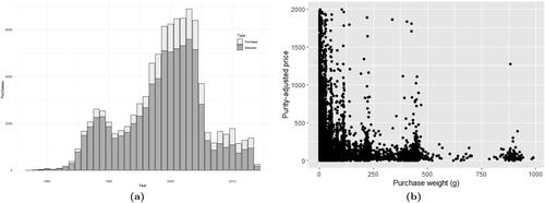
We reran the optimal data aggregation from 1995 through 2013; each year in this period had at least 400 undercover purchases across the US. We lowered our κ to five, a reflection of the lower volume of methamphetamine purchases. Using the data aggregation approach, we found ${\tau }^{*}$ equal to 14 months. Next, using the map in Figure 8 as the source of anecdotal data in the same manner in which we used the map in Figure 3 to ground truth the cocaine analysis, we calibrated the price correlation threshold necessary to infer the presence of a flow and identified a concordance-maximizing value of 0.84, which was used to generate the resulting network shown in Figure 9.

Figure 8. Routes for methamphetamine flows across the US; Source: (USDOJ, 2011).

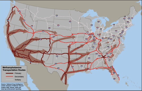
Figure 9. Inferred methamphetamine flows based on the analysis of concordance rates. Flows between observed state-state pairs from the optimal ${\tau }^{*}$ specification are visualized by opaque directed lines.

In the case of the methamphetamine network, the overlap between the generated network and the anecdotal network is 23%. This lower overlap compared to the cocaine network is in part the result of the much higher concordance maximizing correlation threshold (0.84 for methamphetamine vs. 0.57 for cocaine), which produces a sparser set of inferred links (Figure 8) compared with the cocaine network (Figure 3). Both networks show a strong tendency for the drugs to move from the south, southwest, and west in a north and northeasterly direction. Interestingly, we observe a strong tendency for methamphetamine to flow southward from Minnesota, indicating that it is a major distribution center in the Upper Midwest. While it is possible that methamphetamine may be flowing from Canada into Minnesota, it is also linked to California and Texas, both of which are major entry points for methamphetamine into the US (Figure 8). The case of Minnesota is an example of an insight that this kind of analysis can produce that is not available from the anecdotal data.

6.1. Network comparison

The networks for cocaine and methamphetamine consist of the same set of nodes (i.e., the 50 states of the US), making it possible to compare them at the aggregate (network-wide) and node (specific state) level.

Table 3 summarizes selected properties of the methamphetamine flow network. The measure of density, at 4%, is substantially lower than that of the cocaine network (19%, see the comparable Table 2 above), demonstrating that it is even sparser than the cocaine network. A second notable set of differences occurs in the triad census: first, only 18% of all possible triads are non-empty. Perhaps more importantly, only 33% of all triads with two or more edges are out-star to in-star triads. This figure is substantially lower than the analogous figure of 57% for the cocaine network. Since the out-star to in-star triad is a structurally resilient configuration (i.e., the removal of any one edge will not disrupt the flow from the first node to the third node), we can conclude that the cocaine network features more path redundancy at a microstructural level than the methamphetamine network and is therefore more resilient at this level.

Table 3. Aggregate properties of the US methamphetamine flow network. For details on triad census, refer to the online supplement.

Analysis	Property	Measure
Density	Density	4%
Triad census*	Empty subgraph (% of all triads)	16,095 (82%)
	Non-empty triad	3505 (18%)
	Single edge (% non-empty triads)	3038 (87%)
	Out-star (% triads with 2+ edges)	73 (16%)
	In-star (% triads with 2+ edges)	159 (34%)
	Directed line (% triads with 2+ edges)	79 (17%)
	Out-star to in-star (% triads with 2+ edges)	156 (33%)
Core–periphery	Core members	10
	Periphery members	40
	Core density	0.48
	Periphery density	0.01
	Fitness measure	0.61

Another interesting comparison between the cocaine and methamphetamine networks is the core-periphery structure. In both networks, the fitness measure is very similar, as are the measures of density for the core and the periphery. However, unlike the cocaine network, where the core has 21 states, the core for methamphetamine consists of only 10 states (see the online supplement for a complete list), and only three states, Alabama, California, and Indiana, are in the core for both drugs. The anecdotal flow maps in Figures 3 and 8 reveal that California and Alabama are located on major distribution routes in the west and south for both drugs and contain or are in close proximity to multiple arrows. This aligns with their characterization as core members. Although Indiana is located at a distance from the major entry points, both maps show a few large arrows leading into Indiana and an array of small arrows emerging in its neighborhood.

The most noticeable difference between the cocaine and methamphetamine cores is the locations of most core states. As noted above, the cocaine core is concentrated east of the Mississippi River (16 out of 21 states). In contrast, seven of the 10 methamphetamine core states lie to the west of the Mississippi, with a cluster of five of them in the vicinity of the California entry point highlighted in Figure 8. This suggests that, while in the cocaine case a larger number of states farther down the supply chain and presumably closer to end retail markets are well integrated with one another, in the case of the methamphetamine network, the degree of integration is greater closer to the supply side of the market and dissipates as one moves away from this core. One can also speculate that, because methamphetamine is a synthetic drug that can be produced domestically, markets are more localized and fragmented, especially in states located at some distance from a major alternative source of low-cost and smuggled methamphetamine (i.e., Mexico). This is in contrast with cocaine, which, due to its agricultural origins in South America, does not lend itself to domestic production which could act as a substitute for smuggled cocaine.

7. Conclusions

In this article we have demonstrated the feasibility of mapping an illicit drug supply chain network based on the STRIDE data, and we further showed the importance and impact of data aggregation. Key contributions of this article include (i) the novel approach of formulating the data aggregation problem as an optimization problem and (ii) the two-step analytical approach that successfully constructed a network supported by anecdotal evidence, despite the noise and limitations inherent in the data. This method can be used to analyze potentially complementary measures that describe drug flows that may be sparse or noisy. For example, the purity of an illegal drug is recorded in STRIDE. We would expect purity to decrease as it moves along the supply chain as it changes hands and as more opportunities for adulteration take place. In this case, the optimal aggregation can be applied for purity estimation. Similarly, correlated changes in substance abuse treatment admissions and workplace drug testing data both provide measures of drug use prevalence, and patterns of change in these measures may also be useful for network detection.

We particularly note that while the anecdotal data were instrumental in calibrating the correlation threshold used to generate the inferred data, the inferred dataset includes many flows that were not part of the anecdotal dataset, providing a richer portrait of the cocaine trafficking network in the US. By extending our analysis to methamphetamine, we demonstrated that (i) our approach supports not only the analysis of cocaine data but also methamphetamine data, (ii) if similar data for other drugs are available, these methods can be deployed to study those drugs as well, and (iii) comparisons between flow networks of different drugs can be of interest to the drug dependence research and law enforcement communities. In the case of methamphetamine, we found its flow network to be sparser than the cocaine network, with a smaller core of 10 states (compared with 21 for cocaine) and a smaller proportion of resilient triads (i.e., triads within which the removal of one edge is insufficient to disconnect the first node from the last node). All of this suggests that the methamphetamine network is more vulnerable to disruption than the more robust cocaine network.

The two network maps generated in this study can be analyzed in a number of ways, each providing insights that may be of use to law enforcement and drug policy makers and researchers. For example, it would be interesting to identify individual nodes or edges that play a pivotal role in enabling the transportation of cocaine or methamphetamine across the US. Such cut-points or bridges could be important targets for disruption by law enforcement. Identifying source-like nodes (i.e., nodes from which many edges originate) may also provide clues about land, sea, or air border locations that serve as entry points for these drugs into the US, with implications for border interdiction efforts. Overlaying and comparing the cocaine and methamphetamine networks with a view to identifying common edges or subgraphs between them may provide clues about the underlying trafficking organizations that move both products rather than only one, as appears to have increasingly become the case in recent decades. Applying the methods of this article to more granular data or to data for other drugs may provide more spatially precise information or information about flow networks for other drugs.

There are also several interesting potential extensions to the optimization approach presented in this article. First, in this article we limited ourselves to the optimal time aggregation, which does not consider the geospatial dimension. Our approach could be expanded to allow for the aggregation of neighboring locations. Further, we only considered a single fixed aggregation interval. However, one possible extension of our work involves flexible aggregation, meaning that time intervals can be adjusted based on the density of the data in each state or by larger time periods (e.g., if law enforcement activities are non-stationary over the observation period).

The above contributions notwithstanding, it is important to recognize some limitations of our approach. First, because STRIDE undercover purchase data are a product of law enforcement actions, they are a non-random sample of drug market activity, and previous research has demonstrated large within-city variance in prices associated with the quantity transacted and agency involved (Horowitz, 2001; Arkes et al., 2008). Further, only jurisdictions that report both undercover or confidential informant purchases and drug purity enter the data, and those jurisdictions that perform proportionately more purchases are over-represented in the data. If undercover purchases are associated with higher prices, then external validity is limited. We also conduct this analysis at the state level; this masks potentially important within-state heterogeneity, on which more detailed data could shed light.

Lastly, we note that the modern problem of illegal drugs threatens to outmatch traditional data sources and modeling methods. The public health and safety impacts of cocaine and methamphetamine use and their associated illegal markets are immense and evolving, and agencies responsible for law enforcement and interdiction must share and synthesize intelligence from diverse sources across jurisdictions. By varying only the time dimension of the aggregation problem, we demonstrate that an easily replicable method using a single source of data can approximate the combined expert assessment of the intelligence community. The potential applications of these findings are numerous. For example, concordance between the data-generated and the anecdotal network validates qualitative assessments, while strongly positive price correlations estimated by the model highlight potential connections in the network that were previously hidden. By examining changes in model predictions as new data are incorporated, this method can be used to create a dynamic picture of the network as it changes, thereby providing evolving insights leading to efficient ways of disrupting networks that cause enormous societal harm.

Acknowledgments

We thank the anonymous reviewer team for their dedication to the referee process and for their insightful comments and constructive feedback, which significantly shaped the final version of this paper.

Data availability statement

The data that support the findings of this study are available under a Freedom of Information Act request to the United States Drug Enforcement Administration (DEA).

Additional information

Funding

This work was supported by the National Science Foundation under Grant Award ID: 2039862.

Notes on contributors

Margret V. Bjarnadottir

Margret V. Bjarnadottir is an associate professor of management science and statistics at the University of Maryland’s Robert H Smith School of Business. She received her PhD in operations research from MIT’s Operations Research Center, and her undergraduate degree in engineering from University of Iceland. Her research focuses on algorithmic development and data informed decision making in areas of high social impact, including health care and pay equity.

Siddharth Chandra

Siddharth Chandra received a BA degree in economics from Brandeis University, an MA in economics (with PhD pass) from the University of Chicago, and a PhD in economics from Cornell University. At Michigan State University, he is professor of economics in James Madison College, holds a courtesy appointment in the Department of Epidemiology and Biostatistics, and directs the Asian Studies Center. His research interests include behavior and policy relating to addictive substances, pandemics, the intersection of demography, economics, health, and history in Asia, and applications of portfolio theory to fields outside finance, for which the theory was originally developed.

Pengfei He

Pengfei He received a BS degree in statistics from Nankai University in China and an MS degree in statistics from the University of Wisconsin-Madison. He is currently a PhD candidate in computer science at Michigan State University. His research interests include machine learning, adversarial learning and high-dimensional statistics.

Greg Midgette

Greg Midgette received his PhD in public policy analysis from the Pardee RAND Graduate School and MPP from UCLA. He is an assistant professor of criminology at the University of Maryland. His work focuses on policy analysis in the areas of alcohol and drug control, illicit markets, community corrections, and the intersection of public safety and public health.

References

- Arkes, J., Pacula, R.L., Paddock, S.M., Caulkins, J.P. and Reuter, P. (2008) Why the DEA STRIDE data are still useful for understanding drug markets. NBER Working Papers 14224, National Bureau of Economic Research, Inc.
- Benítez, G.J., Chandra, S., Veloza, T.C.L.W.C. and Cárdenas, I.J.D.D. (2019) Following the price: Identifying cocaine trafficking networks in Colombia. Global Crime, 20(2), 90–114.
- Boivin, R. (2014) Risks, prices, and positions: A social network analysis of illegal drug trafficking in the world-economy. International Journal of Drug Policy, 25(2), 235–243.
- Borgatti, S.P., Everett, M.G. and Freeman, L.C. (2002) Ucinet for Windows: Software for Social Network Analysis. Analytic Technologies, Harvard, MA.
- Borgatti, S. and Everett, M. (1999) Models of core/periphery structures. Social Networks, (21), 375–395.
- Caulkins, J.P. (1995, January) Domestic geographic variation in illicit drug prices. Journal of Urban Economics, 37(1), 38–56.
- Caulkins, J.P. (1997, October) Modeling the domestic distribution network for illicit drugs. Management Science, 43(10), 1364–1371.
- Caulkins, J.P. (2007) Price and purity analysis for illicit drug: Data and conceptual issues. Drug and Alcohol Dependence, 90, S61–S68.
- Caulkins, J.P. and Bond, B.M. (2012) Marijuana price gradients: Implications for exports and export-generated tax revenue for California after legalization. Journal of Drug Issues, 42(1), 28–45.
- Caulkins, J.P. and Padman, R. (1993) Quantity discounts and quality premia for illicit drugs. Journal of the American Statistical Association, 88(423), 748–757.
- Caulkins, J.P. and Reuter, P. (1998) What price data tell us about drug markets. Journal of Drug Issues, 28(3), 593–612.
- Chandra, S. and Barkell, M. (2013) What the price data tell us about heroin flows across Europe. International Journal of Comparative and Applied Criminal Justice, 37(1), 1–13.
- Chandra, S., Barkell, M. and Steffen, K. (2011) Inferring cocaine flows across Europe: Evidence from price data. Journal of Drug Policy Analysis, 4(1).
- Chandra, S. and Joba, J. (2015) Transnational cocaine and heroin flow networks in western Europe: A comparison. International Journal of Drug Policy, 26(8), 772–780.
- Chandra, S., Peters, S. and Zimmer, N. (2014) How powdered cocaine flows across the United States: Evidence from open-source price data. Journal of Drug Issues, 44(4), 344–361.
- Cunningham, S. and Finlay, K. (2016) Identifying demand responses to illegal drug supply interdictions. Health Economics, 25(10), 1268–1290.
- Dave, D. (2006, March) The effects of cocaine and heroin price on drug-related emergency department visits. Journal of Health Economics, 25(2), 311–333.
- DeSimone, J. and Farrelly, M.C. (2003, January) Price and enforcement effects on cocaine and marijuana demand. Economic Inquiry, 41(1), 98–115.
- Dobkin, C. and Nicosia, N. (2009) The war on drugs: Methamphetamine, public health, and crime. American Economic Review, 99(1), 324–49.
- Farrell, G., Mansur, K. and Tullis, M. (1996) Cocaine and heroin in Europe 1983-93: A cross-national comparison of trafficking and prices. British Journal of Criminology, 36(2), 255–281.
- Giommoni, L., Aziani, A. and Berlusconi, G. (2017) How do illicit drugs move across countries? A network analysis of the heroin supply to Europe. Journal of Drug Issues, 47(2), 217–240.
- Giommoni, L., Berlusconi, G. and Aziani, A. (2021) Interdicting international drug trafficking: A network approach for coordinated and targeted interventions. European Journal on Criminal Policy and Research, 28(4), 545–572.
- Grossman, M. and Chaloupka, F.J. (1998, August) The demand for cocaine by young adults: A rational addiction approach. Journal of Health Economics, 17(4), 427–474.
- Hayek, F.A. (1945) The use of knowledge in society. The American Economic Review, 35(4), 519–530.
- Horowitz, J. (2001, December) Should the DEAs STRIDE data be used for economic analyses of markets for illegal drugs? Journal of the American Statistical Association, 96, 1254–1271.
- Khavari, B., Sahlberg, A., Usher, W., Korkovelos, A. and Nerini, F.F. (2021) The effects of population aggregation in geospatial electrification planning. Energy Strategy Reviews, 38, 100752.
- Kilmer, B., Everingham, S.M.S., Caulkins, J.P., Midgette, G., Pacula, R.L., Reuter, P., Burns, R.M., Han, B. and Lundberg, R. (2014) What America’s Users Spend on Illegal Drugs: 2000-2010. RAND Corporation, Santa Monica, CA.
- Manski, C.F., Pepper, J.V. and Petrie, C.V. (2001) Informing America’s Policy on Illegal Drugs: What We Don’t Know Keeps Hurting us. National Academies Press, Washington, DC.
- Midgette, G., Davenport, S., Caulkins, J.P. and Kilmer, B. (2019) What America’s Users Spend on Illegal Drugs, 2006-2016. RAND Corporation, Santa Monica, CA.
- Miron, J.A. (2003) The effect of drug prohibition on drug prices: Evidence from the markets for cocaine and heroin. The Review of Economics and Statistics, 85(3), 522–530.
- National Drug Intelligence Center (2002–2004) Narcotics Digest Weekly. U.S. Department of Justice, Washington, DC.
- National Drug Intelligence Center (2006–2011) National Illicit Drug Prices. U.S. Department of Justice, Washington, DC.
- Orcutt, G.H., Watts, H.W. and Edwards, J.B. (1968) Data aggregation and information loss. The American Economic Review, 58(4), 773–787.
- Reuter, P. (1988) Can the Borders Be Sealed? RAND Corporation, Santa Monica, CA.
- Reuter, P. and Kleiman, M.A.R. (1986) Risks and prices: An economic analysis of drug enforcement. Crime and Justice, 7, 289–340.
- Saffer, H. and Chaloupka, F. (1999, July) The demand for illicit drugs. Economic Inquiry, 37(3), 401–411.
- Shellman, S.M. (2004) Time series intervals and statistical inference: The effects of temporal aggregation on event data analysis. Political Analysis, 12(1), 97–104.
- United Nations Office on Drugs and Crime (2018) Transnational organized crime: Let’s put them out of business. Technical report. UNODC. Available at https://www.unodc.org/centralasia/en/news/transnational-organized-crime_-lets-put-them-out-of-business.html
- United Nations Office on Drugs and Crime (UNODC) (2021a) World Drug Report. UNODC. Available at https://www.unodc.org/unodc/en/data-and-analysis/wdr2021.html
- United Nations Office on Drugs and Crime (UNODC) (2021b) The Annual Report Questionnaire. UNODC. Available at https://www.unodc.org/unodc/en/data-and-analysis/arq.html
- United States Department of Justice (2014) System to Retrieve Information from Drug Evidence (STRIDE) database, Wasington DC.
- U.S. Department of Justice (2011) National drug threat assessment 2011, Wasington DC.