Lineaments of Kodaikanal-Palani massif, Southern Granulitic Terrain of Tamil Nadu, India: a study using SRTM DEM and LANDSAT satellite’s OLI sensor’s FCC

Abstract

In the present study an attempt has been made to study the lineaments of the Kodaikanal–Palani massif of Tamil Nadu in southern India. Lineaments extracted from eight different azimuth angles of the SRTM DEM, and Landsat-8 satellite’s OLI sensor’s FCC were integrated to generate a lineament data base for the study area. The extracted lineaments were analysed using ArcGIS and Rockworks software to obtain information regarding the number, length, predominant orientations of lineaments extracted individually from both data, and the final output. These apart spatial variation in lineament density has also been analyzed. Estimations from the final lineament output shows that, 2167 lineaments with their total length being 2997.63 km. Areas of high lineament density are found in the western and north western parts of Kodaikanal Taluk. NE–SW directions are predominant orient direction followed by those orienting in N–S and NW–SE directions, and these orientations are in agreement with the trends of the regional geological structures. Distinct variations in the estimations made of the lineaments extracted from SRTM and OLI data is found to exist. About 40 and 38% of the lineaments of the study area are discernible only in the SRTM data and OLI data, respectively and are not found in each other; only 22% of the lineaments of the study area are found commonly in both the data. Furthermore, NW–SE orienting lineaments are more discernible in SRTM data whereas N–S orienting lineaments are more discernible in OLI data. These variations underlines the fact that lineament mapping using any single data source as has been widely followed will not be adequate to give a reliable picture about the lineaments of an area, and further the study stresses the need to extract lineaments from varied satellite images and integrate them to get a reliable picture of the lineaments.

Keywords:

• Kodaikanal hills
• Palani hills
• lineaments
• SRTM’s DEM
• OLI’s FCC

1. Introduction

The term lineament is defined as a mappable linear or curvilinear feature of a surface whose parts align in a straight or slightly curving relationship that may be the expression of a fault or other linear zones of weakness, as derived from remote sensing sources such as optical imagery, radar imagery or digital elevation models (Sabins, 1996). Understanding of the lineaments of an area can be useful for wide-ranging applications in various fields of geosciences. It was initially used mainly for the exploration of petroleum (Blanchet, 1957; Mollard, 1957) and later its utility expanded to other fields such as groundwater detection, mineral exploration, recognition of geological structures such as folds and faults, identification of seismic prone areas, landslide hazard investigations, landform studies, detection of hot springs, pollution migration and dispersion studies, prediction of possible sites of caves, various fields of civil engineering more commonly in studies pertaining to site selection for the construction of dams, power plants, bridges, roads, etc., and for selection of routes for laying roads and in the selection of areas for new settlements.

Remotely sensed data, both aerial photographs and satellite images have been used extensively to extract lineaments. While aerial photographs were widely used in the initial years, satellite images have become the most common data source since the last two decades towards extracting the lineaments. Sensor data such as Enhanced Thematic Mapper (ETM), ETM⁺, (Panchromatic) PAN, Advanced Spaceborne Thermal Emission and Reflection Radiometer (ASTER) and Shuttle Radar Topography Mission (SRTM) have been widely used for the purpose. For extracting lineaments from these sensor data a number of manual, semi-automatic and automatic techniques are employed and in recent years a number of automated lineament extraction techniques are being used. Some of these techniques include Hough Transform (Argialas & Mavrantza, 2004; Wang et al., 1990), Lineament Extraction and Stripe Statistical Analysis (Zlatopolsky, 1992), Segment Tracing Algorithm (Ni, Zhang, Liu, Yan, & Li, 2016), Haar Transform (Majumdar & Bhattacharya, 1988; Porwik & Lisowska, 2004), Lineament Extraction algorithm of PCI Geomatica software (Hubbard et al., 2012). For the analysis of the extracted lineaments Geographical Information System (GIS) technique has become a powerful and an indispensible tool in view of its ability to process quickly, store results quantitatively and also to generate maps which facilitate the study of their spatial distribution.

2. The study area and its geological setting

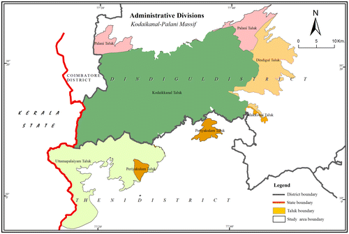
The study area, Kodaikanal–Palani massif, located in the south central part of Tamil Nadu State in India is geographically situated between north latitudes 9°54′56′′–10°29′06′′ and east longitudes 77°12′03′′–77°49′56′′ (Figure 1), and forms part of the Survey of India’s topographic sheets 58 F/4, 7, 8, 11, 12, 15 and 58 G/5 of 1:50,000 scale. Most part of the study area except the southern part lies in the Kodaikanal Taluk of Dindigul District (Figure 2). The southern part lies in Theni District (confining to a portion of Uttamapalaiyam and Periyakulam Taluks). The study area is bounded by the Kerala State on its west, Palani and Dindigul Taluks of Dindigul District on the north and east, respectively, and, Periyakulam and Uttamapalaiyam Taluks of Theni District of Tamil Nadu State on the South. The areal extent of the study area is 1682.87 sq. km. The study area has attracted the attention of geoscientists (Thanavelu, 2012), in view of the frequent landslides that occurs in the study area especially during the rainy season.

Figure 1. Study area. Source: Information Obtained from Survey of India Open Series Map.

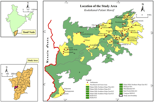
Figure 2. Administrative divisions. Source: Compiled information obtained from Survey of India Open Series Map and Taluk map published by Government of Tamil Nadu.

The region in which the study area is located is referred as Southern Granulitic Terrain (SGT) and is composed of a number of crustal blocks of which the study area forms part of the largest block of them viz., the Madurai crustal block (Meert et al., 2010). This crustal block underwent extensive deformation and metamorphosed to granulite facies during the Neoproterozoic (Bartlett, Harris, Dougherty, Hawkesworth, & Santhosh,1998; Cenki et al., 2004; Santosh, Tanaka, Yokoyama, & Collins, 2005). The study of the ultrahigh-temperature metamorphic assemblages from a number of localities of this block reveal that the peak conditions inferred for the Ultra High Temperature (UHT) rocks of this crustal block are in the range of 7–11 kbar and 950–1150 °C. The age of this metamorphism has been established as ranging between 600 and 480 Ma (; Braun & Kriegsman, 2003; Clark et al., 2009; Collins, Santosh, Braun, & Clark,2007) demonstrating that this metamorphism was synchronous with the final stages of Gondwana amalgamation (Collins & Pisarevsky, 2005). The age of the Kodaikanal–Palani massif has been estimated to be late Archaean to early Palaeoproterozoic (ca. 2.54–2.43, Bartlett et al., 1998; Brandt et al., 2011; Ghosh et al., 2004).

Information relating to the rock types of the study area was obtained from the Quadrangle map (58 F and G) of 1: 250,000 scales, published by the Geological Survey of India in the year 1989. Charnockite is the predominant rock of the study area (Figure 3) Table 1 covering about 86% (465 sq. km) of the study area. Hornblende biotite gneiss is the other rock which occupy considerable portion, especially in the Palani Taluk that falls within the study area, covering about 11% (192.55 sq. km) of the study area. The other rocks occupy only meagre portion of the study area and these include granite, anorthosite, granite gneiss, basic dyke, calc. granulite, along with calcareous mud and clay, laterite and aeolian sands. Of these rocks the oldest rock in the study area is calc. granulite. Younger to this rock is the charnockite which is predominantly garnet-free consisting of hypersthene, biotite, plagioclase, perthite and quartz. The charnockites of the study area are of intermediate composition with a tonalitic to granitic affinity (Valdiya, 2016). Later tectonic activity and metamorphism has led to the retrogression of the granulites, giving rise to granitic gneiss (which are confined to the western part of the study area) and hornblende biotite gneiss (which are found in the northern and western margins of the study area). Extensive migmatization, presumably during the orogenic period was marked by emplacement of later intrusive of granite, the remnants of which are confined to the western parts of the study area. Anorthosite is confined to the north east margin and it occurs as elliptical body closely associated with the charnockites. Linear dykes of doleritic composition are found to occur within the hornblende biotite gneissic areas especially in the north eastern part of the study area. All the above described rocks are of Archaean age. These apart, calc. mud and clay, and laterites of Tertiary age also occur but are limited in areal extent. Aeolian sands are of Quaternary age are also found and are restricted to a portion of the Uttamapalaiyam Taluk in the southern part of the study area. A major shear zone viz., the Karur–Kambam–Painavu–Trichur Shear Zone (KKPTSZ) cuts through the study area in a nearly NE–SW direction (Brandt et al., 2011; Plavsa et al., 2012; Shazia et al., 2015; Singh et al., 2006).

Figure 3. Rock types. Source: Information obtained from published geology map by Geological Survey of India.

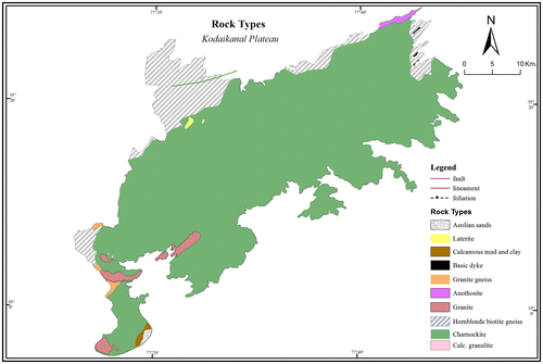
Table 1. Rock types of the study area and their areal extent.

Sl. No.	Rock types	Area (in sq. km)	Area (in %)
(1)	Aeolian sands	2.83	0.17
(2)	Laterite	1.76	0.10
(3)	Calcareous mud and clay	3.84	0.23
(4)	Basic dyke	0.86	0.05
(5)	Granite gneiss	5.72	0.34
(6)	Anorthosite	6.06	0.36
(7)	Granite	27.20	1.62
(8)	Hornblende biotite gneiss	192.55	11.44
(9)	Charnockite	1441.79	85.67
(10)	Calc. granulite	0.26	0.02
Total		1682.87	100.00

3. Methodology

The present study has been accomplished in three stages where in the first stage, literature relevant to the present study which includes those relating to the various aspects of lineaments, rock types, geological structure and tectonic history of the study area were collected, compiled and reviewed. This has been done to have a thorough understanding of the theme under study. The second stage pertains to the extraction of lineaments. Shuttle Radar Topographic Mission (SRTM) satellite data and Landsat-8 satellite’s OLI sensor data, both of 9 May 2016, were freely downloaded from the website – http://earthexplorer.usgs.gov/ for the purpose. The SRTM satellite data was made use of to generate Digital Elevation Model (DEM) to facilitate the extraction of lineaments for the study. The DEM offers visual perspective capability, accentuation of terrain features, and application of the three-dimensional analysis system, and as such, it avoids the problem associated with the lack of stereo coverage in the imagery. Topographic features which represent lineaments such as straight valleys, continuous scraps, straight streams segments and rock boundaries, systematic off set of streams, sudden tonal variations and alignment of vegetation were visually interpreted and digitized on screen. Such extraction of lineaments of the study area was carried out in eight different azimuth angles (45°, 90°, 135°, 180°, 225°, 270°, 315° and 360°) in order to facilitate their extraction to the maximum possible extent. Furthermore, interpretation of lineaments at each of these azimuth angles was done at two different scales (1:50,000 and 1:80,000 scales) to ensure mapping of lineaments of all sizes. The extracted lineaments from each azimuth angle were compared with other data sources such as topographic maps, high resolution Google images, etc., to eliminate non-geological lineaments. This elimination of non-geological lineaments was performed for all the eight lineament maps extracted from the eight different azimuth angles. After this elimination process, rest of the other lineaments in each of the eight different azimuth angles was stored in eight different separate GIS shape files. This was followed by combining all the lineaments obtained from these eight different shape files into a single shape file. From this output the redundant/duplicate lineaments were eliminated and the merged SRTM lineament output of the study area was generated and was kept ready for the analysis. This was followed by the generation of False Colour Composite (FCC) from the Landsat-8 satellite’s OLI sensor data. This OLI sensor’s FCC image was visually interpreted onscreen for lineaments, and after eliminating non-geological linear such as roads, topographic ridges, agricultural field boundaries, etc., the lineament map was finalized (Figure 6). In the next stage, the lineaments extracted from these two different data sets (SRTM DEM MERGED output and OLI’s FCC image) were merged together into a single output. During this process, redundant or duplicate lineaments were eliminated. This output has been referred in the text as the final lineament output. In the next stage estimations such as number of lineaments, length of lineaments and lineament density were made using Arc GIS software. Orientation of the lineaments of the study area was also analyzed using Rockworks software – 2016 version (www.rockwork.com), one of the most commonly used software for the purpose. All these estimations and analysis were done for all the eight different azimuth angles and their merged output of the SRTM data, OLI’s FCC image and for the final lineament output. The results of the analysis are discussed in the following section.

4. Results

Estimations regarding the number of lineaments in the study area from the SRTM DEM data (in eight different azimuth angles and their merged output), FCC data of the OLI sensor, and, the final lineament output (which includes the final merged output of the SRTM DEM and the OLI sensor’s FCC image) were made. The total number of lineaments in the study area compiled from all eight azimuth angles of the SRTM DEM merged output is 1351. Amongst the eight different azimuth angles, the maximum number of lineaments (701 lineaments) was extracted from the 45° azimuth angle output, whilst the least number of lineaments (363) was extracted from 225° azimuth angle. The numbers of lineaments extracted from other azimuth angles were within these two extremes. In case of OLI sensor’s FCC image, lineaments were extracted only from one azimuth angle as there is no option for viewing it in different azimuth angles unlike SRTM DEM, and the number of lineaments extracted from it is 1307. The final lineament output generated after merging the lineaments from the merged output (1351 lineaments) of SRTM data and the OLI sensor’s FCC image (1307 lineaments), and eliminating the redundant lineaments (491) is found to consist of 2167 lineaments.

Estimations regarding the length of lineaments in the study area from the SRTM DEM image (in eight different azimuth angles Figure 4(a)–(h) and final merged output Figure 4(i)), FCC data of the OLI sensor Figure 5, and, the final lineament output Figure 6 were made (Table 2) using ArcGIS software. The total length of lineaments in the study area compiled from all eight azimuth angles of the SRTM DEM merged output is 1820.05 km. However the number of lineaments extracted from each of the eight different azimuth angles varied from 585.99 km (225° azimuth angle) to 881.52 km (45° azimuth angle). In case of FCC generated from the OLI sensor image the total length of lineaments extracted from it is 1772 km. The total length of lineaments from the final lineament output is 2997.63 km.

Figure 4. (a) Lineaments extracted by 45° Azimuth angle. (b) Lineaments extracted by 90° Azimuth angle. (c) Lineaments extracted by 135° Azimuth angle. (d) Lineaments extracted by 180° Azimuth angle. (e) Lineaments extracted by 225° Azimuth angle. (f) Lineaments extracted by 270° Azimuth angle. (g) Lineaments extracted by 315° Azimuth angle. (h) Lineaments extracted by 360° Azimuth angle. (i) Dem merged output. Source: (a-h) Shuttle Radar Topography mission Satellite's DEM Data obtained from Online Resources and (i) Generated from Shuttle Radar Topography mission Satellite's DEM Data.

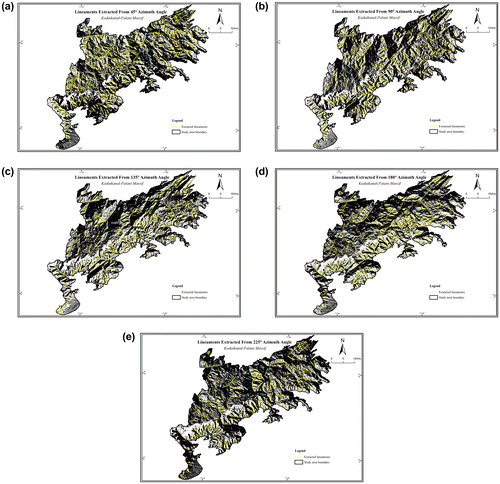
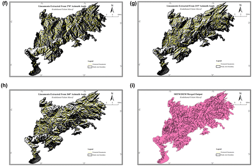
Figure 5. Lineaments extracted from Lansat OLI. Source: From Landsat 8 Satellite's OLI Sensor obtained from Online Resources.

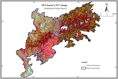
Figure 6. Final output. Source: Generated both from SRTM and Landsat 8 OLI satellite images.

Table 2. Total number of lineaments in SRTM DEM image.

Sl. No.	Angles (in degrees)	SRTM DEM
		Total numbers	Total length (in km)
(1)	45	701	881.52
(2)	90	398	701.62
(3)	135	400	687.57
(4)	180	436	744.59
(5)	225	363	585.99
(6)	270	464	621.81
(7)	315	372	627.57
(8)	360	414	614.41
(9)	Merged	1351	1820.05

Based on the length of the lineaments, the extracted lineaments were classified into very short (<1 km.), short (1–2 km), medium (2–3 km), long (3–4 km) and very long (>4 km) lineaments. Estimations show that in case of the merged output of SRTM DEM, very short and short lineaments are found to be more in number with 602 and 544 lineaments, respectively, constituting about 85% of the total number of lineaments of the study area. Medium sized and longer lineaments constitute about 9 and 4% of the total lineaments, respectively, while very long lineaments are few in number (27), constituting just 2% of the total number of lineaments of the study area. In case of OLI sensor’s FCC also, very short and short lineaments are predominating, together they constitute about 83% of the total number of lineaments of the study area. Medium sized and longer lineaments constitute about 11 and 4% of the total lineaments, respectively, while very long lineaments are few in number (25), constituting just less than 2% of the total number of lineaments of the study area. Further, in case of the final lineament output also, very short and short lineaments are predominating and they together constitute about 82% of the total number of lineaments of the study area. Medium sized and longer lineaments constitute about 11 and 4% of the total lineaments, respectively, while very long lineaments are few in number (49), constituting just above 2% of the total number of lineaments of the study area.

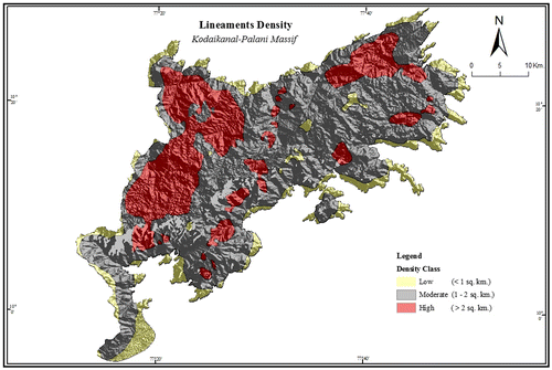
Lineament density is the total length of all lineaments divided by the area under consideration (1 sq. km in the present study). For understanding the spatial variation in lineament density in the study area, a grid of cells, 1 sq. km each was overlaid over the lineament map (Final lineament output) of the study area and the length of lineaments in each grid was estimated (Table 3). Based on the range of the lineament density values of the grids spread over the study area, different lineament density categories were demarcated by drawing isolines. Thus a map showing various lineament density zones was prepared using ArcGIS software and is shown in Figure 7. In the study area lineament density varies from 0 to 4.3 km/sq. km. The study area was demarcated into three different lineament density classes such as low (<1 km/sq. km), moderate (1–2 km/sq. km) and high (>2 km/sq. km). The lineament density is found to be moderate in most part of the study area covering about 61% (1023.82 sq. km) of the study area. It is found to be high in about 26% (435.10 sq. km) of the study area and such high density areas are confined mainly to the three patches, the largest of which is found in the western and north western parts of the study area especially in the western parts of Kodaikanal Taluk (Palani hills Northern Slope West Reserved Forest and Umaiyar Hill Reserved Forest). The other patch, comparatively smaller, is located in the north eastern part of the study area especially in the north eastern part of Kodaikanal Taluk (Palani hills Northern Slope East Reserved Forest. The third patch, a narrow, linear and discontinuous one runs through Kodaikanal town, in the central part of the study area, in a NE–SW direction. Lineament density is found to be low in about 13% of the study area and such low density class is found confined mostly to the fringes of the study area.

Table 3. Lineament density classes and their areal extent.

Lineament density
Sl. No.	Range (km/sq. km)	Density class	Area (in sq. km)	Area (in %)
(1)	<1	Low	223.95	13.31
(2)	1−2	Moderate	1023.82	60.84
(3)	>2	High	435.10	25.85
Total			1682.87	100.00

Figure 7. Lineament density. Source: Generated both from SRTM and Landsat 8 OLI satellite images.

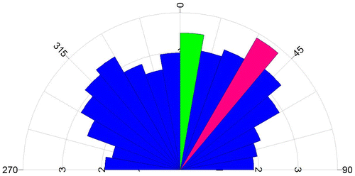
The analysis of rose diagrams constructed for lineament outputs of each of the eight different azimuth angles of the SRTM DEM (Figure 8(a)–(h)) reveals that the lineaments are oriented predominantly in an NE–SW direction in five azimuth angles viz., 90°,135°, 270°, 315° and 360°. Even in case of the other three azimuth angles, NE–SW is one of the predominant orientation of the lineaments, though NW–SE is more predominating in case of 45° and 180° azimuth angles, and nearly N–S orientation in case of 135° and 225°. In case of the merged output (Figure 8(i)), the lineaments are predominantly oriented in NE–SW and NW–SE directions. The lineaments extracted from the OLI sensor image is predominantly oriented in a near N–S direction (Figure 9), and lineaments oriented in NE–SW direction are next in importance. From the analysis of rose diagram constructed for the final output (Figure 10), it is observed that the lineaments of the study area are oriented in diverse directions. However those orienting in NE–SW directions are found to be predominant, followed by N–S and NW–SE orienting lineaments.

Figure 8. (a–h) Orientation of lineaments extracted from SRTM DEM. (i) Orientation of lineaments – from the merged output of SRTM DEM.

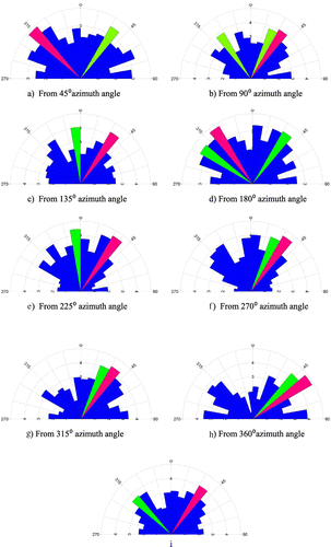
Figure 9. Orientation of lineaments extracted – from Landsat-8 Satellite’s OLI sensor’s FCC.

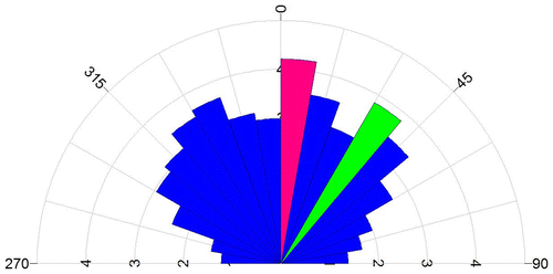
Figure 10. Orientation of lineaments (both from SRTM DEM and OLI sensor’s FCC).

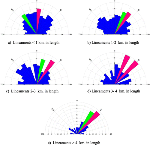
Rose diagrams constructed to understand the existence of any size-wise preferred orientation(s) of lineaments in the study area, reveal that in case of the merged output of SRTM DEM, very short lineaments are found to be dominantly oriented in three directions, viz., NE–SW, NW–SE and near N–S directions (Figure 11). The shorter lineaments are predominantly oriented in NE–SW direction (Figure 11(b)). In case of moderate-sized lineaments two distinct preferred orientations (NE–SW and near N–S) was observed (Figure 11(c)). The longer and very longer lineaments are found to be predominantly oriented in NNE–SSW (Figure 11(d)) and NE–SW (Figure 11(e)) directions, respectively. Lineaments extracted from the OLI sensor’s FCC image shows that very short lineaments are predominantly oriented in two directions viz., near N–S and NNW–SSE directions (Figure 12(a)). The shorter lineaments are predominantly oriented in NE–SW direction (Figure 12(b)). The moderate-sized lineaments are predominantly oriented in three directions viz., NE–SW, near N–S and NW–SE directions (Figure 12(c)) while the longer lineaments are predominantly oriented in NE–SW direction (Figure 12(d)). Very long lineaments are also oriented predominantly in NE–SW in addition to ENE–WSW direction (Figure 12(e)). In case of the final lineament output of the study area, very short lineaments are predominantly oriented in a near N–S direction (Figure 13(a)). All the other sized lineaments are predominantly oriented in a NE–SW direction (Figure 13(b)–(e)). The moderate-sized lineaments in addition to the NE–SW direction are also predominantly oriented in NNE–SSW direction.

Figure 11. Orientation of lineaments of varied sizes extracted from SRTM DEM.

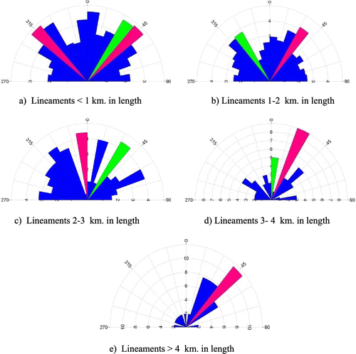
Figure 12. Orientation of lineaments of varied sizes extracted from Landsat-8 Satellite’s OLI sensor.

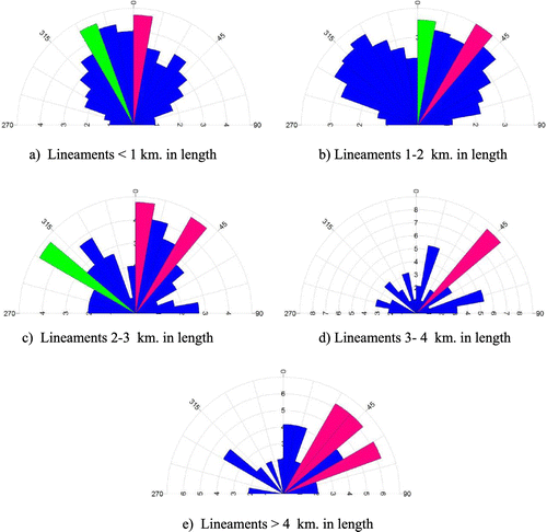
Figure 13. Orientation of lineaments of varied sizes: SRTM DEM + Landsat-8 Satellite’s OLI sensor.

5. Discussion

Estimation of the number of lineaments from the final lineament output has shown that altogether there are 2167 lineaments of varied sizes in the study area. In case of SRTM DEM’s merged output it is 1371 whereas it is slightly less (1307) in case of OLI sensor’s FCC. This in spite of the fact that while the lineaments of the merged output of the SRTM data is a compilation of lineaments extracted from eight different azimuth angles, whereas the lineaments of the OLI sensor’s FCC is only from one azimuth angle. This is due to the reason that linear vegetation patterns are easily detectable in FCC and are less discernible in DEM. In addition the shadow effect in DEM obscures the detection of these lineaments posing limitations in mapping lineaments. Though a glance at the number of lineaments extracted from these two different data sources seems less, a deeper analysis reveals interesting facts. During the process of compiling all the lineaments extracted from both the merged SRTM DEM and OLI sensor’s FCC data towards generating the final lineament output, it was observed there were 491 (i.e., 22.66% of the total lineaments) redundant lineaments i.e., found in both the data. The remaining 860 lineaments (39.69%) extracted from SRTM DEM data is exclusively extractable only from it and is not identifiable in OLI’s FCC. Similarly the remaining 816 lineaments (37.66%) extracted from OLI’s FCC are exclusively extractable only from it and is not identifiable in ASTER DEM output. This clearly shows that lineament extraction from any one data source will be grossly insufficient to get a complete picture of the lineaments of an area. Further, analysis of the number of lineaments from various azimuth angle reveal that the number of lineaments extractable varies widely in different azimuth angles. Extraction of lineaments was relatively easier from the 45° azimuth angle output as the maximum number of lineaments was extracted from this output. But even from this output the proportion of the lineaments extracted from this azimuth angle is only 52% of the total lineaments of the merged SRTM data, and in case of other azimuth angles, the proportion is still lesser. This underlines the inadequacy of extracting lineaments from any single azimuth angle, which has been the common practice in mapping lineaments from DEM generated from SRTM/ASTER satellite images. Similar view has been put forth by Jawahar Raj et al. (2017) from the study of lineaments of the neighbouring Kolli hills. Furthermore, the study stresses the need to extract lineaments from such DEMs from as many azimuth angles as possible to get a more reliable picture. The above discussion clearly brings to light the fact that lineaments identifiable at an azimuth angle or a particular sensor may not be apparent in another azimuth angle or in another sensor. Hence mapping of lineaments from any single satellite image/product may be inadequate to provide a reliable picture on the number of lineaments of an area. This stresses the need to make use of a variety of satellite data as possible to enhance the identification of lineaments.

Analysis of the length of the lineaments from the final lineament output reveals that the total length of lineaments from the final lineament output is 2997.63 km. The length of lineaments extracted from OLI sensor’s FCC is 1772 km, which is only slightly lesser than the length (1820.05 km) extracted from the merged output of SRTM DEM. This in spite of the fact that while the lineaments of the merged output of the SRTM data is a compilation of lineaments extracted from eight different azimuth angles, the lineaments of the OLI sensor’s FCC is only from one azimuth angle. These variations in the length of lineaments extracted from varied sources reinforces the suggestion put forth, that any one satellite image may not be adequate to map the lineaments of an area, and as many varied data should be utilized to get a reliable picture about the lineaments of an area. Further, the analysis of the length of lineaments extracted from the eight azimuth angles of the SRTM DEM data reveals that the length is maximum in 45° azimuth angle output but still it constitutes only about 48.43% of the total length of lineaments of the study area, obtained from the merged SRTM DEM output. This underlines the inadequacy of extracting lineaments from any single azimuth angle, which has been the common practice in mapping lineaments from satellite image. Furthermore, the study stresses the need to extract lineaments from as many azimuth angles as possible to get a more reliable picture.

Amongst the varied sizes of the lineaments, the very short and short lineaments are found to be predominant (constituting 82% of the total lineaments) as revealed from the analysis of the estimation of the number of lineaments of varied sizes from the final lineament output. In case of the SRTM DEM merged output and OLI’s FCC also very short and short lineaments are predominant and their proportion is almost similar (85 and 83%, respectively). This clearly shows the remarkable consistency in the proportion of very short and short lineaments irrespective of the data used towards the extraction of lineaments.

The lineament density map prepared from the final lineament output reveal that in the study area, lineament density is high in areas closer to the KKPTSZ, the major shear zone of the region. Also the lineament density maxima axis is parallel to the orientation of the trend of the KKPTSZ. In view of the lineament density’s direct relationship with degree of rock fracturing (Edet et al., 1998)/shearing (Chandrasekhar et al., 2011), permeability of rocks (Masoud & Koike, 2011), groundwater yield from wells (Sener et al., 2005), degree of hazardness especially relating to slope failures (Kiran & Ahmed, 2014), etc., it can be concluded that in the areas of high lineament density of the study area viz., Palani hills Northern Slope West Reserved Forest, Palani hills Northern Slope East Reserved Forest and Umaiyar Hill Reserved Forest areas, the degree of rock deformation is likely to be high with the resultant higher degree of rock fracturing and shearing making these areas unsuitable for the construction of dams and reservoirs as the possibility of water leakages into the subsurface, slope and dam failures and rate of sedimentation would be high. However, these areas could be targeted for groundwater exploitation.

The analysis of predominant orientation(s) of the lineaments of the study area (as inferred from the final lineament output) shows that the lineaments of the study area are oriented in diverse directions reflecting the multiple episodes of deformation events that have occurred in the region through geologic time (Bartlett, Harris, Hawkesworth, & Santhosh,1995; Chetty & Bhaskar Rao, 2006; Drury & Holt, 1980; Geological Survey of India, [GSI], 2006; Jayananda et al., 1995; Unnikrishnan-Warrier et al., 1995). However amongst these diverse orientations, the lineaments orienting in NE–SW directions are predominant, followed by those orienting in N–S and NW–SE directions. All these three orientations (besides ENE-WSW) are the predominating orientations of the lineaments of the Indian Subcontinent (Rakshit & Prabhakar Rao, 1989), and also the Tamil Nadu State (Geological Survey of India, 2006). The predominant orientation of the lineaments (NE–SW) of the study area corresponds well with the orientation of the KKPTSZ, the major shear zone that passes through the study area. Thus the results of the analysis of the predominant orientations of the study area is in agreement with the results of previous studies conducted pertaining to this region and with prominent geological structures of the study area.

A comparative analysis of the predominant orientation(s) of lineaments extracted from the SRTM DEM and OLI sensor’s FCC data show that while the lineaments extracted from SRTM DEM data are found to be oriented predominantly in NE–SW direction followed by NW–SE direction, the lineaments extracted from OLI sensor image are found to be oriented predominantly in a near N–S direction followed by NE–SW direction. These results show that the NE–SW orienting lineaments are easily identifiable in both the data whereas the NW–SE orienting lineaments and N–S orienting lineaments are more discernible in SRTM DEM data and OLI sensor’s FCC data, respectively.

The analysis of the orientation of lineaments of varied sizes, shows that in the study area the predominant orientation of the lineaments of varied sizes deduced from the final lineament output is found to be NE–SW direction, with the exception of very short lineaments which are predominantly oriented in a near N–S direction. Comparison of the predominant orientations of lineaments of varied sizes extracted from SRTM DEM and OLI sensor’s FCC shows that in general NE–SW orienting lineaments are predominating irrespective of lineament size with the exception of very short lineaments where distinct difference in their predominant directions exists in both the data. While in case of SRTM DEM, their predominant orientation is NE–SW, this direction is insignificant in case of OLI sensor’s FCC where they are predominantly oriented in a near N–S and NNW-SSE directions. This clearly reflects the easy identification of NE–SW orienting shorter lineaments from SRTM DEM data, and also the easy identification of near N–S, and NNW-SSE orienting shorter lineaments from OLI sensor’s FCC. The results once again underlines the fact that lineament mapping using any single data like SRTM DEM /ASTER DEM/SWIR/FCC as has been widely followed will not be adequate to give a reliable picture about the lineaments of an area, and further stresses the need to extract lineaments from varied satellite images to get a reliable picture of the lineaments.

6. Conclusion

The present study provides a new lineament database including the number and length of lineaments, lineament density, predominant orientation of lineaments for the Kodaikanal–Palani massif which could useful for several applications including developmental and management planning of the hills. It has also demonstrated the inadequacy of mapping lineaments from any single satellite data as has been widely adopted and strongly underlines the need to extract lineaments from a variety of satellite data to get a more reliable picture about the lineaments of the area under study.

Disclosure statement

No potential conflict of interest was reported by the authors.

References

- Argialas, D. P., & Mavrantza, O. D. (2004, July 12–23). Comparison of edge detection and Hough transform techniques for the extraction of geologic features. In O. Altan (Ed.), Proceedings XXth ISPRS Congress of the International Society of Photogrammetry and Remote Sensing, Istanbul, Turkey. ISPRS Archives XXXV (Part B3), (pp. 790–795). Retrieved from http://www.isprs.org/proceedings/XXXV/congress/comm3/papers/376.pdf
- Bartlett, J. M., Harris, N. B. W., Hawkesworth, C. J., & Santhosh, M. (1995). New isotope constraints on the crustal evolution of South India and pan-African granulite metamorphism. Memoir of Geological Society of India, 34, 391–397.
- Bartlett, J. M., Harris, N. B. W., Dougherty, Jon S., Hawkesworth, C. J., & Santhosh, M. (1998). The application of single zircon evaporation and model Nd ages to the interpretation of polymetamorphic terrains: an example from the Proterozoic mobile belt of south India. Contributions to Mineralogy and Petrology, 131(2–3), 181–195.
- Blanchet, P. H. (1957). Development of fracture analysis as exploration method. Bulletin of the American Association of Petroleum Geologists, 41(8), 1748–1759.
- Brandt, S., Schenk, V., Raith, M. M., Appel, P., Gerdes, A., &Srikantappa, C. (2011). Late neoproterozoic P-T evolution of HP-UHT granulites from the palni hills (South India): New constraints from phase diagram modelling, LA-ICP-MS zircon dating and in situ EMP monazite dating. Journal of Petrology, 52, 1813–1856. doi:10.1093/petrology/egr032
- Braun, I., & Kriegsman, L. M. (2003). Proterozoic crustal evolution of southernmost India and Sri Lanka. Geological Society, London, Special Publications, 206, 169–202.10.1144/GSL.SP.2003.206.01.10
- Cenki, B., Braun, I., & Brocker, M. (2004). Evolution of the continental crust in the Kerala Khondalite Belt, southernmost India: Evidence from Nd isotope mapping, U–Pb and Rb–Sr geochronology. Precambrian Research, 134, 275–292.10.1016/j.precamres.2004.06.002
- Chandrasekhar, P., Martha, T. R., Venkateswarlu, N., Subramanian, S. K., & Kamaraju, M. V. V. (2011). Regional geological studies over parts of Deccan Syneclise using remote sensing and geophysical data for understanding hydrocarbon prospects. Current Science, 100(1), 95–99.
- Chetty, T. R. K., & Bhaskar Rao, Y. J. (2006). Constrictive deformation in transpressional regime, field evidence from the Cauvery Shear Zone, Southern Granulite Terrain, India. Journal of Structural Geology, 28, 713–720.10.1016/j.jsg.2006.01.007
- Clark, C., Collins, S., Timms, N. E., Kinny, P. D., Chetty, T. R. K., &Santhosh, M. (2009). SHRIMP U–Pb age constraints on magmatism and high-grade metamorphism in the Salem Block, southern India. Gondwana Research, 16, 27–36.10.1016/j.gr.2008.11.001
- Collins, A. S., Santosh, M., Braun, I., & Clark, C. (2007). Age and sedimentary provenance of the Southern Granulites, South India: U– Th–Pb SHRIMP secondary ion mass spectrometry. Precambrian Research, 155, 125–138.
- Collins, A. S., & Pisarevsky, S. A. (2005). Amalgamating eastern Gondwana: The evolution of the Circum-Indian Orogens. Earth-Science Reviews, 71, 229–270.10.1016/j.earscirev.2005.02.004
- Drury, S. A., & Holt, R. W. (1980). The tectonic framework of the South Indian craton: A reconnaissance involving LANDSAT imagery. Tectonophysics, 65, T1–T15.10.1016/0040-1951(80)90073-6
- Edet, A. E., Okereke, C. S., & Esu, E. O. (1998). Applications of remote sensing data to groundwater exploration: A case study of the Cross River State, SE Nigeria. Hydrogeology Journal, 6, 394–404. doi:10.1007/s100400050162
- Geological Survey of India. (2006). Geology and mineral resources of the states of India Tamil Nadu and Pondicherry ( Miscellaneous Publication No. 30). G.S.I, Chennai, 71p.
- Ghosh, J. G. Wit, M. J. D., Zartman, R. E. (2004). Age and tectonic evolution of neoproterozoic ductile shear zones in the Southern Granulite Terrain of India with implications for Gondwana Studies. Tectonics, 23, TC3006.
- Hubbard, B. E., Mack, T. J., & Thompson, A. L. (2012). Lineament analysis of mineral areas of interest in Afghanistan (28 p). U.S. Geological Survey Open-File Report 2012–1048.
- Jayananda, M., Janardhan, A. S., Sivasubramanian, P., & Peucat, J. J. (1995). Geochronologic and Isotopic constraints on granulite formation in the Kodaikanal area, Southern India. Memoir Geological Society of India, 34, 373–390.
- Jawahar Raj, N., Prabhakaran, A., & Muthukrishnan, A. (2017). Extraction and Analysis of Geological Lineaments of Kolli Hills, Tamil Nadu: A study using remote sensing and GIS. Arabian Journal of Geosciences, 10, 195. doi:10.1007/s12517-017-2966-4
- Kiran, Raj S., & Ahmed, S. A. (2014). Lineament extraction from Southern Chitradurga Schist belt using Landsat TM, ASTERGDEM and geomatics techniques. International Journal of Computer Applications, 93(12), 12–20.
- Majumdar, T. J., & Bhattacharya, B. B. (1988). Application of the Haar transform for extraction of linear and anomalous patterns over part of Cambay Basin, India. International Journal of Remote Sensing, 9(12), 1937–1942.10.1080/01431168808954992
- Masoud, A., & Koike, K. (2011). Auto-detection and integration of tectonically significant lineaments from SRTM DEM and remotely-sensed geophysical data. ISPRS Journal of Photogrammetry and Remote Sensing, 66, 818–832.10.1016/j.isprsjprs.2011.08.003
- Meert, J. G., Pandit, M. K., Pradhan, V. R., Banks, J., Sirianni, R., Stroud, M.,Newstead, B., & Gifford, J. (2010). Precambrian crustal evolution of Peninsular India: A 3.0 billion year odyssey. Journal of Asian Earth Sciences, 39, 483–515.10.1016/j.jseaes.2010.04.026
- Mollard, J. D. (1957). Aerial photographs aid petroleum search. Candian Oil and Gas Industries, 10(7), 89–96.
- Ni, C.Z., Zhang, S., Liu ,C., Yan, Y., & Li, Y. (2016). Lineament length and density analyses based on the segment tracing algorithm: A case study of the Gaosong Field in Gejiu Tin Mine, China. Mathematical Problems in Engineering. Article ID 5392453, 1–7, doi:10.1155/2016/5392453
- Plavsa, D., Collins, A. S., Foden, J. F., Kropinski, L., Santosh, M., Chetty,T. R. K., & Clark, C. (2012). Delineating crustal domains in Peninsular India: Age and chemistry of orthopyroxene-bearing felsic gneisses in the Madurai Block. Precambrian Research, 198–199, 77–93.
- Porwik, P., & Lisowska, A. (2004). The Haar-Wavelet transform in digital image processing: Its status and achievements. Machine Graphics & Vision, 13(1–2), 79–98.
- Rakshit, A. M., & Prabhakar Rao, P. (1989). Megalineaments on the face of the Indian sub-continent and their geological significance. Memoirs of Geological Sur vey of India, 12, 17–24.
- Sabins, F. F. (1996). Remote sensing: Principles and interpretation (3rd ed., 494p). New York, NY: W. H. Freeman and Company.
- Santosh, M., Tanaka, K., Yokoyama, K., & Collins, A. S. (2005). Late Neoproterozoic Cambrian felsic magmatism along transcrustal shear zones in southern India: U-Pb electron microprobe ages and implications for the amalgamation of the Gondwana supercontinent. Gondwana Research, 8, 31–42.
- Sener, E., Davraz, A., & Ozcelik, M. (2005). An integration of GIS and remote sensing in groundwater investigations: A case study in Burdur, Turkey. Hydrogeology Journal 13: 826–834.10.1007/s10040-004-0378-5
- Shazia, J. R., Harlov, D. E., Suzuki, K., Kim, S. W., Girish-Kumar, M.,Hayasaka, Y., Ishwar-Kumar, C., Windley, B. F., & Sajeev, K. (2015). Linking monazite geochronology with fluid infiltration and metamorphic histories: Nature and experiment. Lithos, 236–237, 1–15. doi:10.1016/j.lithos.2015.08.008
- Singh, A. P., Kumar, N., , & Singh, B. (2006). Nature of the crust along Kuppam–Palani geotransect (South India) from gravity studies: Implications for Precambrian continental collision and delamination. Gondwana Research, 10, 41–47.10.1016/j.gr.2005.11.013
- Thanavelu, C. (2012). Landslide hazard zonation on macroscale of Kodaikanal hills, Dindigul district, Tamil Nadu. Records of the Geological Survey of India, 144 (5), 233.
- Unnikrishnan-Warrier, C., Santosh, M., & Yoshida, M. (1995). First report of Pan-African Sm—Nd and Rb—Sr mineral isochron ages from regional charnockites of southern India. Geological Magazine, 132(3), 253–260.10.1017/S0016756800013583
- Valdiya, K. S. (2016). The making of India: Geodynamic evolution (2nd ed., 924p). Switzerland: Springer. 10.1007/978-3-319-25029-8
- Wang, P. J., & Howarth, P. J. (1990). Use of the Hough transform in automated lineament detection. IEEE Transactions on Geoscience and Remote Sensing, 28(4), 561–567.10.1109/TGRS.1990.572949
- Zlatopolsky, A. A. (1992). Program LESSA (lineament extraction and stripe statistical analysis) automated linear image features analysis – Experimental results. Computers and Geosciences, 18(9), 1121–1126.10.1016/0098-3004(92)90036-Q