Prediction of the sodium absorption ratio using data-driven models: a case study in Iran

ABSTRACT

In this investigation, two data-driven models, i.e., Gaussian Process (GP) and Support Vector Machine (SVM), were used to predict the sodium absorption ratio (SAR) in three sub-watersheds (Khorramabad, Biranshahr, and Alashtar) in Iran. A comparison was also done with these data-driven models with Artificial Neural Network (ANN). The parameters total dissolved solids, electrical conductivity, pH value, CO₃, HCO₃, chlorine (Cl), SO₄, calcium (Ca), magnesium (Mg), sodium (Na), and potassium (K) were used as input variables and SAR as output. For SVM and GP regression, two kernel functions (radial-based kernel and Person VII kernel function) were used. The results from this investigation suggest that the ANN model (correlation coefficient [CC], root mean square error [RMSE], Nash–Sutcliffe coefficient of efficiency [NSC], and mean absolute relative error [MARE] = 0.9966, 0.0286, 0.9906, and 0.0194) is more precise as compared to the GP (CC, RMSE, NSC, and MARE = 0.9570, 0.2982, 0.8288, and 0.3705) and SVM (CC, RMSE, NSC, and MARE = 0.9948, 0.0365, 0.9847, and 0.063). Among GP and SVM, SVM with PUK kernel is more accurate for estimating the SAR of the watershed. Thus, ANN is a technique which could be used for predicting the SAR for given study area.

KEYWORDS:

• Sodium absorption ratio
• Gaussian Process
• Support Vector Regression
• Artificial Neural Network

Introduction

Freshwater is the essential and finite resource for agriculture, human being, and industries. Sustainable development of any country or area totally depends upon freshwater. It could not be possible without adequate quality and quantity of freshwater. Water quality control and assessment is the major issue in the water resource planning and management (Bartram & Ballance, 1996). It is the most important part of operation and design of the irrigations system. Corp pattern is also decided by it in any region (Suarez, 1981). In the last few decades, urbanization and industrialization are at its peak. With the increase of the industrialization and urbanization, the quality and quantity of the freshwater decrease. A large amount of domestic and industrials waste are being dumped into the freshwater resources (Palmer, 2001), which results to the generation of a large amount of the wastewater or conversion of freshwater into waste, ultimately enters into the irrigation system and affects the crop productivity of any region.

Sodium absorption ratio (SAR) of the irrigation water is one of the major and common indicators on which the suitability of the irrigation water depends (Sposito & Mattigod, 1977). The SAR indicator is calculated by measuring the concentrations of sodium, calcium, and magnesium in water used for irrigation (Weiner, 2012). Presence of higher values of sodium decreases the infiltration rate of soil, reduces the stability of the soil, and increases the sodium accumulation in leaf tissue (Micke, 1996) and gave poisonous effects to the crops. The normal soil may convert in the saline soil by using the sodium affected water for irrigation purpose (Saha et al., 2017).

The higher the concentration of sodium, the lower the hydraulic conductivity and infiltration rate of soil and it decreases to such a level that minimum amount of water reached to the plant crop and ultimately reduce the crop yield (Bouwer & Idelovitch, 1987). The excess amount of SAR also affected the leaf of the crop such as stone fruits, avocado, and almond (Bouwer & Idelovitch, 1987). Higher SAR also affected the permeability of the soil. The dispersion of the soil particles occurred due to exchangeable sodium present in the soil which replaces the magnesium and calcium absorbed in the soil clay (Asadollahfardi, Khodadadi, & Gharayloo, 2010). Ayers and Tanji (1981) studied the SAR and categorized the hazardous effect of the SAR into three categories: (1) if the value of SAR below is 3 then no sodium problems, (2) if in between 3 and 9 then less sodium problems, and (iii) if above 9 then higher the sodium problems.

Various researchers have been used various data mining and data-driven techniques in civil and environmental engineering applications (Mehdipour, Stevenson, Memarianfard, & Sihag, 2018; Nain, Sihag, & Luthra, 2018; Parsaie, 2016; Parsaie, Azamathulla, & Haghiabi, 2018; Parsaie & Haghiabi, 2017, 2015; Parsaie, Najafian, Omid, & Yonesi, 2017; Sihag, 2018; Sihag, Singh, Vand, & Mehdipour, 2018a; Sihag, Tiwari, & Ranjan, 2018b, 2017; Singh, Sihag, & Singh, 2017; Singh, Sihag, Singh, & Kumar, 2018; Tiwari, Sihag, Kumar, & Ranjan, 2018; Vand, Sihag, Singh, & Zand, 2018). Asadollahfardi, Hemati, Moradinejad, and Asadollahfardi (2013) used ANN to predict the SAR in which Na, Mg, Ca, SO₄, Cl, HCO⁻₃, pH were input variables and SAR was output and found that ANN has the capability to predict the SAR accurately and precisely. Sattari, Pal, Mirabbasi, and Abraham (2018) predict the SAR using M5P model tree regression and found encouraging performance of data-driven model. Sihag, Singh, Gautam, and Debnath (2018c) used various data-driven models to predict the infiltration characteristics and found these techniques work exceptionally well. Keeping it in the view, the objective of this investigation is to predict the SAR of three watersheds in Iran (Khorramabad, Piranshahr, and Alashtar) by using two kernel functions (RBF and PUK) of Gaussian Process (GP) and Support Vector Regression (SVM). Furthermore, the results were also compared with the Artificial Neural Network (ANN) model.

Data-driven techniques

GP regression

GP regression relies upon the postulation that nearby observation must share the information mutually and it’s an approach of mentioning earlier straight over the function space. The simplification of Gaussian distribution is known as Gaussian regression. The matrix and vector of Gaussian distribution are expressed as covariance and mean in GP regression. Due to having earlier knowledge of function reliance and data, the validation for generalization is not essential. The GP regression models are capable of recognizing the foresee distribution consequent to the input test data (Rasmussen & Williams, 2006).

A GP is the collection of number of random variable, any finite number of them has a collective multivariate Gaussian distribution. Assume u and v stand for input and output domain accordingly, thereupon x pairs (g_i, h_i) are drawn freely and equivalently for distribution. For regression, it is assumed that h ⊆ R_e, then a GP on p is expressed by the mean function v₀: u, R_e and covariance function µ: u × u, R_e. Readers are requested to follow the Kuss (2006) to get the exhaustive details of GP.

SVM

This method was first proposed by Vapnik (1998) and based on statistical learning theory or VC theory. The present form of the SVM was developed by the Vapnik and coworker at AT&T laboratory (Boser, Guyon, & Vapnik, 1992). The main principle of SVM is the optimal separation of classes. From the separable classes, SVM selects the one which have lowest generalization error from infinite number of linear classifier or set upper limit to error which is generated by structural risk minimization. This way the maximum margin between two classes can be found from the selected hyper plane and sum of distances of the hyper plane from the nearby point of two classes will set highest margin between two classes. Readers are requested to follow the Smola (1996) to get the exhaustive details of SVM. Cortes and Vapnik (1995) give the idea of kernel function for nonlinear support vector regression. The main idea of SVM is to minimize error, individualizing the hyperplane which maximizes the margin, keeping in mind that part of the error is tolerated. The main advantage of the SVM is that it can be used to avoid difficulties of using linear functions in the high dimensional feature space and optimization problem is transformed into dual convex quadratic programs. The flowchart of the SVM is discussed in Figure 1.

Figure 1. Details of the SVM.

ANN

ANN is one of the most used data-driven techniques and inspired by the functioning of nervous system and brain architecture (Haykin, Haykin, Haykin, & Haykin, 2009). ANN has one input, one or more hidden, and one output layer. Each layer consists of number of nodes and the weighted connection between these layers represents the link between nodes. Input layer having nodes equal to the number of input parameters distributes the data presented to the network and doesn’t help in processing. This layer follows one or more hidden layer which helps in processing of data. The output layer is final processing unit. When an input layer is subjected to an input value which passes through the interconnections between nodes, these values are multiplied by the corresponding weight and summed to obtain the net output (z_j) to the unit

(1) $z_j=\sum _i{W}_{ij}\times y_i$(1)

where W_ij is weigh of interconnection from unit i to j, y_i is the input value at input layer, z_j is output obtained by activation function to produce an output for unit j. The detailed discussion about NN is provided (Haykin 1999). In present analysis, a three-layer feed forward multilayer perceptron ANN based on the back propagation algorithm is used.

SAR calculation

The SAR was calculated for these three watersheds by using the following formula (U. S. Salinity Laboratory Staff, 1954):

(2) $\mathrm{S}\mathrm{A}\mathrm{R}=\frac{(\mathrm{N}{\mathrm{a}}^{+})}{\sqrt{\frac{1}{2}\left[\left(\mathrm{M}{\mathrm{g}}^{2+}\right)+(\mathrm{C}{\mathrm{a}}^{2+}\right)]}}$(2)

where Na⁺, Mg²⁺, and Ca²⁺ are in milli equivalents per liter (mEq/l).

Study area and dataset

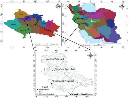
The study area (Khorram Abad, Piranshahr, and Alashtar sub-watersheds) covers a part of Lorestan province located in the center of Iran (Figure 2). They are part of Karkheh River basin (Persian Gulf drainage basin). The study area is located between 33°11′47″ N and 34°03′27″ N, and between 48°03′10″ E and 48°59′07″ E. Sub-watersheds are defined according to the position of sampling site and cover an area of 3576 km² as shown in Figure 2. The area is a part of the semiarid region and has a mean annual rainfall of about 400 mm with the highest precipitation occurring in January and February. Elevation varies from 1158 to 3646 m a.s.l. The upper part of the study area is mountains built mainly of Cretaceous and Miocene limestone and the lower part is alluvial plain. Dataset consists of 775 datasets (training and testing) of the water quality for the three watersheds (Alsthar, Piranshahr, and Khoramabad) in Iran from May 1971 to May 2017. The parameters which were studied during this investigation are total dissolved solids, electrical conductivity, pH value, CO₃, HCO₃, chlorine (Cl), SO₄, calcium (Ca), magnesium (Mg), sodium (Na), potassium (K), and SAR, whereas SAR used as a output variable and remaining all as the input variables. Table 1 shows the characteristics of the parameters in training and testing stage. The values of the SAR lie in between 0.029 and 2.44. Hence, if the values of the SAR are below 3, then it didn’t create any serious problem to the crop and agriculture system (Ayers & Tanji, 1981).

Table 1. Characteristics of the dataset used in this study.

Variables	Minimum	Maximum	Mean	Standard error	Standard deviation	Kurtosis	Skewness	Sample variance
Training dataset
TDS (mg/l)	112	484	240.164	3.108	68.721	−0.453	0.334	4722.604
Ec	178	745	373.204	4.827	106.751	−0.478	0.363	11,395.794
PH	5.2	8.44	7.830	0.018	0.404	4.605	−1.701	0.163
CO3 (meq/l)	0	0.6	0.050	0.005	0.103	5.752	2.318	0.011
HCO3 (meq/l)	0.9	5	3.072	0.038	0.839	−0.883	−0.040	0.704
Cl (meq/l)	0.08	2.6	0.345	0.008	0.180	51.180	4.657	0.032
SO4 (meq/l)	0.01	2.25	0.351	0.014	0.299	6.431	2.094	0.089
Ca (meq/l)	0.9	4.1	2.442	0.036	0.791	−1.197	−0.058	0.625
mg (meq/l)	0.09	4	1.106	0.025	0.562	4.723	1.727	0.315
na (meq/l)	0.03	2	0.224	0.007	0.164	34.076	4.318	0.027
K (meq/l)	0	3.05	0.036	0.007	0.146	370.268	18.125	0.021
SAR	0.029	1.754	0.246	0.008	0.169	18.823	3.159	0.029
Testing dataset
TDS (mg/l)	40	663	362.688	5.885	99.346	0.449	0.547	9869.645
Ec	260	1020	564.484	8.835	149.144	0.381	0.685	22,243.997
PH	6	8.69	7.727	0.030	0.498	0.512	−0.912	0.248
CO3 (meq/l)	0	1.4	0.064	0.009	0.156	20.820	3.684	0.024
HCO3 (meq/l)	1.25	6.6	3.981	0.064	1.085	−0.583	−0.069	1.178
Cl (meq/l)	0.1	3.3	1.109	0.022	0.380	3.759	0.905	0.144
SO4 (meq/l)	0	2.77	0.565	0.027	0.458	3.145	1.489	0.210
Ca (meq/l)	0.95	5.6	2.982	0.056	0.949	−0.566	−0.155	0.901
mg (meq/l)	0.6	5.7	1.840	0.041	0.697	3.393	1.339	0.486
na (meq/l)	0.06	2.8	0.841	0.025	0.419	0.548	0.352	0.175
K (meq/l)	0	1.13	0.080	0.009	0.144	34.504	5.227	0.021
SAR	0.059	2.44	0.80	0.025	0.418	0.203	0.279	0.175
Total dataset
TDS (mg/l)	40	663	285.279	3.613	100.520	0.823	0.805	10,104.362
Ec	178	1020	443.637	5.556	154.562	0.803	0.809	23,889.259
PH	5.2	8.69	7.792	0.016	0.444	2.415	−1.354	0.197
CO3 (meq/l)	0	1.4	0.055	0.004	0.125	20.824	3.477	0.016
HCO3 (meq/l)	0.9	6.6	3.407	0.037	1.034	−0.341	0.271	1.069
Cl (meq/l)	0.08	3.3	0.626	0.016	0.457	1.811	1.277	0.209
SO4 (meq/l)	0	2.77	0.431	0.014	0.380	5.345	1.937	0.144
Ca (meq/l)	0.9	5.6	2.641	0.032	0.891	−0.703	0.066	0.794
mg (meq/l)	0.09	5.7	1.376	0.025	0.709	2.811	1.317	0.503
na (meq/l)	0.03	2.80	0.451	0.015	0.412	1.669	1.424	0.170
K (meq/l)	0	3.05	0.052	0.005	0.147	237.489	13.102	0.022
SAR	0.02	1.725	0.318	0.010	0.278	1.574	1.395	0.077

Figure 2. Locations of the study area.

Detail of kernel functions for SVM and GP

The SVM and GP-based regression approaches design includes the scheme of kernel function (Pal & Deswal, 2011; Rasmussen & Williams, 2006). There are several kernel functions in GP and SVM. In this study, two kernel functions were used with GP and SVM technique.

1. Radial basis kernel (RBF) = $e^{-\gamma {\left|a-b\right|}^2}$

2. Pearson VII function kernel (PUK) $\begin{array}{l}=\\ {\left(1/\left[1+{\left(2{\sqrt{\Vert a-b\Vert }}^2\sqrt{2^{\left(1/\omega \right)}-1}/\sigma \right)}^2\right]\right)}^{\omega }\end{array}$ (Üstün, Melssen, & Buydens, 2006)

where γ, $\sigma$, and $\omega$ are kernel parameters. It is well known that GP and SVM estimation performance depends on a good setting of meta-parameters, Gaussian noise, C, γ, $\sigma$, and ω. The selections of Gaussian noise, C, γ, $\sigma$, and ω control the prediction (regression) model complexity. In this study, a physical method was used to select primary parameters (i.e., C, γ, $\sigma$, $\omega$, and Gaussian noise). In order to minimize the RMSE and to maximize the correlation coefficient (CC), suitable values of various primary parameters are selected. The same kernel-specific parameters were taken for GP regression and as well as for SVM.

Statistical performance evaluation criteria

CC, RMSE, Nash–Sutcliffe coefficient of efficiency (NSC), and mean absolute relative error (MARE) values were calculated to investigate the performance of GP, SVM, and ANN techniques.

CC

The CC is computed as

(3) $CC=\frac{m{\sum }_{i=1}^m{o}_i{t}_i-\left({\sum }_{i=1}^m{o}_i\right)\left({\sum }_{i=1}^m{t}_i\right)}{\hspace{0.17em}\sqrt{m{\sum }_{i=1}^m\left({o_i}^2\right)-{\left({\sum }_{i=1}^m{o}_i\right)}^2}\hspace{0.17em}\sqrt{m{\sum }_{i=1}^m\left({o_i}^2\right)-{\left({\sum }_{i=1}^m{t}_i\right)}^2}\hspace{0.17em}}\hspace{0.17em}$(3)

RMSE

The RMSE is computed as

(4) $\mathrm{R}\mathrm{M}\mathrm{S}\mathrm{E}=\sqrt{\frac{1}{m}(\sum _{i=1}^m{\left(o_i-t_i\right)}^2}$(4)

NSC

The NSC (Nash & Sutcliffe, 1970) is computed as

(5) $\mathrm{N}\mathrm{S}\mathrm{C}=1-\frac{\sum _{i=1}^m{\left(o_i-t_i\right)}^2}{\sum _{i=1}^m{\left(o_i-\overline{o_i}\right)}^2}$(5)

MARE

The MARE is computed as

(6) $\mathrm{M}\mathrm{A}\mathrm{R}\mathrm{E}=\frac{1}{m}\left|\sum _{i=1}^m\frac{o_i-t_i}{o_i}\right|$(6)

where $o_i$ = calculated values of SAR, $t_i$ = estimated values of SAR, m = number of observations, and $\overline{o_i}$ = mean calculated values of the SAR.

Results and discussions

Results of GP

The user-defined functions for the GP are Gaussian noise, γ, σ, and ω and finding of the user-defined functions is trial and error process using Weka (3.9). RBF and PUK are two kernel functions which were used in this investigation. The values of the user-defined function for GP are summarized in Table 2. The values of the Gaussian noise are kept constant for both the kernel.

Table 2. Details of the user-defined functions for GP.

Kernel function	User-defined functions
RBF kernel	Gaussian noise = 1, $\gamma$ = 0.8
PUK kernel	Gaussian noise = 1, $\omega$ = 0.8, $\sigma$ = 6.8

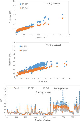
Table 3 furnished the performance of the GP model using performance evaluation parameters (CC, RMSE, MARE, and NSC). It is found in Table 3 that the values of the performance evaluation parameters for the PUK kernel (CC, RMSE, NSC, and MARE 0.9570, 0.2982, 0.8288 and 0.3705, respectively) are much better than RBF kernel (CC, RMSE, NSC, and MARE 0.8931, 0.1870, 0.5988, and 0.2385) with testing dataset. Figure 3 gave the details of the performance of the GP model. Outcomes from Table 3 and Figure 3 show that PUK kernel gave the excellent result as compare to the RBF kernel. Hence, GP with PUK kernel was selected for further comparison.

Table 3. Performance of GP.

	Training dataset				Testing dataset
Approaches	CC	RMSE	NSC	MARE	CC	RMSE	NSC	MARE
GP_RBF	0.9761	0.0379	0.8993	0.1806	0.8931	0.1870	0.5988	0.2385
GP_PUK	0.9340	0.0723	0.6338	0.4511	0.9570	0.2982	0.8288	0.3705

Bold values provide the most precise values of the performance evaluation parameters

Figure 3. Performance of the GP model.

Result of SVM

The user-defined functions for the SVM are C, γ, σ, and ω and finding of the user-defined functions is also a trial and error process using Weka 3.9. In SVM also, two kernel functions (RBF and PUK kernel) are used. Table 4 gave the values of the user-defined functions for SVM model.

Table 4. Details of the user-defined functions for SVM.

Kernel function	User-defined functions
RBF kernel	C = 3, $\gamma$ = 0.8
PUK kernel	C = 3, $\omega$ = 0.8, $\sigma$ = 6.8

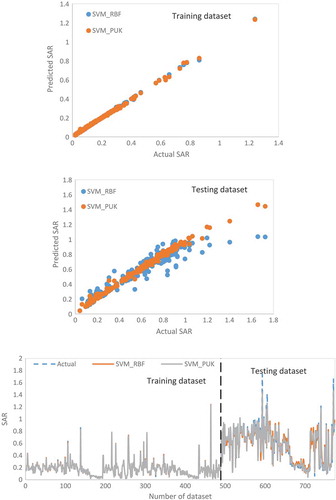
Table 5 summarized the performance of the SVM model using two performance evaluation parameters, i.e., CC and RMSE. It is clear from Table 4 that SVM with PUK kernel gave good result as compared to the SVM with RBF. The values of CC, RMSE, NSC, and MARE for PUK and RBF were 0.9948, 0.0365, 0.9847, and 0.063 and 0.9509, 0.0992, 0.8873, and 0.1328 with testing dataset. Figure 4 gave the details of the performance of the GP model. Outcomes from Table 5 and Figure 4 show that results of SVM with PUK kernel were superior to RBF kernel. Hence, SVM with PUK kernel was selected for further comparison.

Table 5. Performance of SVM.

	Training dataset				Testing dataset
Approaches	CC	RMSE	NSC	MARE	CC	RMSE	NSC	MARE
SVM_RBF	0.9995	0.0038	0.9989	0.0163	0.9509	0.0992	0.8873	0.1328
SVM_PUK	0.9993	0.0047	0.9984	0.0190	0.9948	0.0365	0.9847	0.063

Bold values provide the most precise values of the performance evaluation parameters

Figure 4. Performance of the SVM model.

Comparison of results

In this section, the comparison was done of the best-selected kernel function of SVM and GP model with ANN model. Same like GP and SVM, the modelling of ANN was done with Weka 3.9 and user-defined functions for this model are momentum, learning rate, hidden layers, and iterations. The values of the these user-defined functions were found out by trial and error process and values of these parameters were 0.3, 0.2, 5, and 3000 for momentum, learning rate, hidden layers, and iterations, respectively.

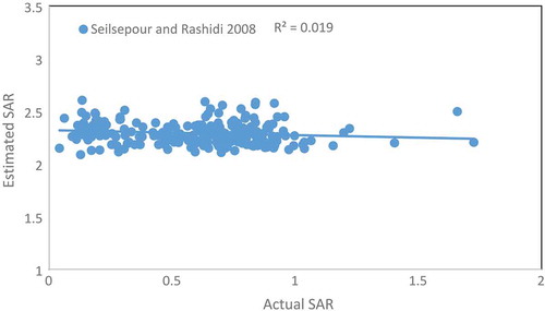
Table 6 gave the details of the performance of the ANN and the best-selected kernel of SVM and GP model. ANN model gave the maximum values of CC and minimum values of the RMSE among all the models. The values of the CC, RMSE, NSC, and MARE with ANN model were 0.9966, 0.0286, 0.9906, and 0.0194, respectively, using testing dataset. Figure 5 gave the performance of the ANN model and the best-selected kernel of GP and SVM model. It is clear from the outcomes of Figure 5 that the output of the ANN model follows the same trends as the actual values of the SAR. Hence, the ANN model is the most accurate to predict the SAR for the given study area. Further, the best fitted model (ANN) was compared to with the recent study (Seilsepour & Rashidi, 2008). But the performance of the Seilsepour and Rashidi model was very poor. The values of RMSE and CC for this model were 1.758142 and −0.13783, respectively. Figure 6 gave the performance of the Seilsepour and Rashidi model with R² value 0.019. Therefore, ANN is the best model among the data-driven model and recent studies.

Table 6. Performance of ANN and best-selected kernel of SVM and GP.

	Training dataset				Testing dataset
Approaches	CC	RMSE	NSC	MARE	CC	RMSE	NSC	MARE
ANN	0.9999	0.0015	0.9998	0.0098	0.9966	0.0286	0.9906	0.0194
GP_PUK	0.9340	0.0723	0.6338	0.4511	0.9570	0.2982	0.8288	0.3705
SVM_PUK	0.9993	0.0047	0.9984	0.0190	0.9948	0.0365	0.9847	0.063

Bold values provide the most precise values of the performance evaluation parameters

Figure 5. Performance of the ANN model and best-selected kernel of GP and SVM model.

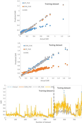
Figure 6. Performance of Seilsepour and Rashidi model to predict the SAR.

Conclusions

The SAR is the indicator which used to find out the suitability of the irrigation water for the crops and possible hazards to the soil. In this investigation, two data-driven models GP and SVM (two kernels each, i.e., RBF and PUK) were used to predict the SAR; further results were compared with the third most used data-driven method (ANN). Obtained results concluded that the ANN model is the most efficient model to predict the SAR than GP and SVM for given study area. Among SVM and GP, the SVM model gave highly precise result than GP. Similarly, among the kernel function, the PUK kernel gave the better result than the RBF for both the techniques model. Seilsepour and Rashidi model was also failed to predict the SAR. Thus, ANN model was the most suitable model for predicting the SAR for the given study area.

Disclosure statement

No potential conflict of interest was reported by the author.

References

- Asadollahfardi, G., Hemati, A., Moradinejad, S., & Asadollahfardi, R. (2013). Sodium adsorption ratio (SAR) prediction of the Chalghazi river using artificial neural network (ANN) Iran. Current World Environment, 8(2), 169–178.
- Asadollahfardi, G., Khodadadi, A., & Gharayloo, R. (2010). The assessment of effective factors on Anzali wetland pollution using artificial neural networks. Asian Journal of Water Environment and Pollution, 7(2), 23–30.
- Ayers, R. S., & Tanji, K. K. (1981). Agronomic aspects of crop irrigation with wastewater. Proceedings of the Specialty Conference, Water Forum ’81, San Francisco, 578–586.
- Bartram, J., & Ballance, R., World Health Organization. (1996). Water quality monitoring: A practical guide to the design and implementation of freshwater quality studies and monitoring programs. UNEP/WHO
- Boser, B. E., Guyon, I. M., & Vapnik, V. N. (1992). A training algorithm for optimal margin classifiers. In Proceedings of the fifth annual workshop on Computational learning theory(pp. 144-152). ACM.
- Bouwer, H., & Idelovitch, E. (1987). Quality requirements for irrigation with sewage water. Journal of Irrigation and Drainage Engineering, 113(4), 516–535.
- Cortes, C., & Vapnik, V. (1995). Support-vector networks. Machine Learning, 20(3), 273–297.
- Haykin, S. (1999). Multilayer perceptrons. Neural networks. A Comprehensive Foundation, 2, 156–255.
- Haykin, S. S., Haykin, S. S., Haykin, S. S., & Haykin, S. S. (2009). Neural networks and learning machines (Vol. 3). Upper Saddle River: Pearson.
- Kuss, M. (2006). Gaussian process models for robust regression, classification, and reinforcement learning. Doctoral dissertation, Ph.D. thesis, Technische Universität, Darmstadt, 189.
- Mehdipour, V., Stevenson, D. S., Memarianfard, M., & Sihag, P. (2018). Comparing different methods for statistical modeling of particulate matter in Tehran, Iran. Air Quality, Atmosphere & Health, 11(10), 1155-1165.
- Micke, W. C. (1996). Almond production manual (Vol. 3364). California: University of California, Division of Agriculture and Natural Resources.
- Nain, S. S., Sihag, P., & Luthra, S. (2018). Performance evaluation of fuzzy-logic and BP-ANN methods for WEDM of aeronautics super alloy. MethodsX, 5, 890–908.
- Nash, J. E., & Sutcliffe, J. V. (1970). River flow forecasting through conceptual models part I—A discussion of principles. Journal of Hydrology, 10(3), 282–290.
- Pal, M., & Deswal, S. (2011). Support vector regression based shear strength modelling of deep beams. Computers & Structures, 89(13–14), 1430–1439.
- Palmer, M. D. (2001). Water quality modeling: A guide to effective practice. Washington, DC: World bank publications.
- Parsaie, A. (2016). Predictive modeling the side weir discharge coefficient using neural network. Modeling Earth Systems and Environment, 2(2), 63.
- Parsaie, A., Azamathulla, H. M., & Haghiabi, A. H. (2018). Prediction of discharge coefficient of cylindrical weir–Gate using GMDH-PSO. ISH Journal of Hydraulic Engineering, 24(2), 116-123.
- Parsaie, A., & Haghiabi, A. (2015). The effect of predicting discharge coefficient by neural network on increasing the numerical modeling accuracy of flow over side weir. Water Resources Management, 29(4), 973–985.
- Parsaie, A., & Haghiabi, A. H. (2017). Improving modelling of discharge coefficient of triangular labyrinth lateral weirs using SVM, GMDH and MARS techniques. Irrigation Drainage, 66(4), 636–654.
- Parsaie, A., Najafian, S., Omid, M. H., & Yonesi, H. (2017). Stage discharge prediction in heterogeneous compound open channel roughness. ISH Journal of Hydraulic Engineering, 23(1), 49–56.
- Rasmussen, C. E., & Williams, C. K. (2006). Gaussian processes for machine learning (Vol. 1, pp. 248). Cambridge: MIT Press.
- Saha, J. K., Selladurai, R., Coumar, M. V., Dotaniya, M. L., Kundu, S., & Patra, A. K. (2017).oil and its role in the ecosystem. In Saha J. K. et al. (Eds.), Soil pollution – an emerging threat to agriculture (pp. 11–36). Singapore: Springer.
- Sattari, M. T., Pal, M., Mirabbasi, R., & Abraham, J. (2018). Ensemble of M5 model tree based modelling of sodium adsorption ratio. Journal of AI and Data Mining, 6(1), 69–78.
- Seilsepour, M., & Rashidi, M. (2008). Modeling of soil sodium adsorption ratio based on soil electrical conductivity. ARPN Journal of Agricultural and Biological Science, 3(5&6), 27–31.
- Sihag, P. (2018). Prediction of unsaturated hydraulic conductivity using fuzzy logic and artificial neural network. Modeling Earth Systems and Environment, 4(1), 189-198.
- Sihag, P., Singh, B., Gautam, S., & Debnath, S. (2018c). Evaluation of the impact of fly ash on infiltration characteristics using different soft computing techniques. Applied Water Science, 8(6), 187.
- Sihag, P., Singh, B., Vand, A. S., & Mehdipour, V. (2018a). Modeling the infiltration process with soft computing techniques. ISH Journal of Hydraulic Engineering, 1–15.
- Sihag, P., Tiwari, N. K., & Ranjan, S. (2017). Prediction of unsaturated hydraulic conductivity using adaptive neuro-fuzzy inference system (ANFIS). ISH Journal of Hydraulic Engineering, 1–11.
- Sihag, P., Tiwari, N. K., & Ranjan, S. (2018b). Support vector regression- based modeling of cumulative infiltration of sandy soil. ISH Journal of Hydraulic Engineering, 1–7.
- Singh, B., Sihag, P., & Singh, K. (2017). Modelling of impact of water quality on infiltration rate of soil by random forest regression. Modeling Earth Systems and Environment, 3(3), 999–1004.
- Singh, B., Sihag, P., Singh, K., & Kumar, S. (2018). Estimation of trapping efficiency of vortex tube silt ejector. International Journal of River Basin Management, 1–38.
- Smola, A. J. (1996). Regression estimation with support vector learning machines ( Doctoral dissertation, Master’s thesis, Technische Universität München).
- Sposito, G., & Mattigod, S. V. (1977). On the chemical foundation of the sodium adsorption ratio 1. Soil Science Society of America Journal, 41(2), 323–329.
- Suarez, D. L. (1981). Relation between pHc and sodium adsorption ratio (SAR) and an alternative method of estimating SAR of soil or drainage waters1. Soil Science Society of America Journal, 45(3), 469–475.
- Tiwari, N. K., Sihag, P., Kumar, S., & Ranjan, S. (2018). Prediction of trapping efficiency of vortex tube ejector. ISH Journal of Hydraulic Engineering, 1–9.
- U. S. Salinity Laboratory Staff, L. A. Richards, ed. (1954). Diagosis and improvement of saline and alkali soil(p. 60). U. S. Department of Agriculture Handbook.
- Üstün, B., Melssen, W. J., & Buydens, L. M. (2006). Facilitating the application of support vector regression by using a universal pearson VII function based kernel. Chemometrics and Intelligent Laboratory Systems, 81(1), 29–40.
- Vand, A. S., Sihag, P., Singh, B., & Zand, M. (2018). Comparative evaluation of infiltration models. KSCE Journal of Civil Engineering, 22(10), 4173-4184.
- Vapnik, V. (1998). Statistical learning theory. New York: Wiley.
- Weiner, E. R. (2012). Applications of environmental aquatic chemistry: A practical guide. Florida: CRC press.