Model-based soil temperature estimation using climatic parameters: the case of Azerbaijan Province, Iran

ABSTRACT

Estimating soil temperature (ST) profile is identified as essential knowledge for plants, crop growth, and germination in all agriculture regions. In this study, daily soil temperature (DST) was modeled using Multilayer perceptron (MLP) model, Gaussian Process (GP), Random Forest (RF), and the M5P model methods for estimating and comparing DST in arid regions. The data selected to test the proposed models are obtained from two stations in Tabriz and Ahar, located in the Azerbaijan province of Iran. Input dataset includes air temperature, relative humidity, wind speed, and sunshine as dependent parameters, whereas ST at depths of 5 cm was selected for the target in model development. The results show the MLP works better than GP-, RF-, and M5P-based models in estimating the DST, with excellent performance indicators such as the mean absolute error, root mean square error, and coefficient of correlation. Results showed that the MLP model with RMSE = 3.2626°C was more suitable than other models in ST estimation 2 days ahead for Tabriz station. Also, in Ahar, MLP with RMSE = 6.3332°C was more suitable than GP-, RF-, and M5P-based models for estimating DST. As a conclusion, the developed MLP is recommended for estimating the DST profiles.

KEYWORDS:

• Daily soil temperature
• Multilayer perceptron model
• Gaussian Process
• Random Forest
• M5P model

1. Introduction

Climatic and weather conditions are dependent upon several factors among which soil temperature (ST) is an essential parameter in exchanging the heat and energy between soil surface and atmosphere. The information about ST is needed for many agricultural (agronomy, soil science) and engineering applications (geo-technology, hydrology, meteorology, ecology, and environmental studies). Moreover, it assists agronomists and engineers to decide the proper plantation date, design drainage and irrigation systems, and optimum utilization of pesticides and fertilizers to reduce chemical pollution of soils and groundwater (Singh, 2000; Sun et al., 2012). Mutually with chemical and physical features of soil organic material, ST is one of the main parameters contributing to the biological activity of soil (Kätterer & Andrén, 2009), e.g., soil respiration, microbial decomposition, organic matter storage, and mineralization, etc. (Öztürk, Atsan, Polat, & Kara, 2011). Soil thermal conditions largely affect the plant growth and agricultural crop yield, due to which, in many cases, ST has relatively higher importance than surface air temperature (Hillel, 1998).

Atluri, Hung, and Coleman (1999) designed an artificial neural network (ANN) for the classification of soils and predicted soil moisture and temperature based on remotely sensed data. Forecasting and simulations related to temporal and spatial predictions of ST received much attention in recent years due to the development and usage of the latest modeling methods and software. Due to seldom availability of comprehensive ST data (Schaetzl, Knapp, & Isard, 2005) and difficulties in spatial measurement (Kang, Kim, Oh, & Lee, 2000) regarding the frequent collection of large-scale data, forecasting of ST needs to be estimated from other informative metrological variables using theoretical, empirical, or soft computing models.

Bilgili (2010) investigated the potential of regression and multilayer perceptron model (MLP) models in estimating ST using climate data (atmospheric pressure, solar radiation, and atmospheric temperature) in the Adana, Turkey and observed that MLP model has higher performance than the regression models. Öztürk et al. (2011) choose meteorological data of different stations to estimate STs using ANN model and found very satisfactory results. Wu et al. (2013) implemented the MLP and indicated MLP as a capable tool for estimation of STs. Kim and Singh (2014) also suggested that adaptive neuro-fuzzy inference system (ANFIS) and ANN models as an efficient tool for estimating STs at different depths.

Talaee (2014) estimated daily soil temperature (DST) using coactive neuro-fuzzy inference system (CANFIS) for semi-arid and arid areas. The DST data were collected from two metrological places at six different levels. The satisfactory performance of the CANFIS is reported for both areas. Kisi, Tombul, and Kermani (2015) compared different methods and models including generalized regression neural networks, radial basis neural networks, and MLP neural networks to estimate STs by using meteorological data. Nahvi, Habibi, Mohammadi, Shamshirband, and Al Razgan (2016) have forecasted DST using self-adaptive evolutionary extreme learning machine for six different soil depths. Data were collected from two metrological stations (Kerman and Bandar Abbas in Iran). They selected meteorological parameters (global solar radiation, atmospheric pressure, and air temperature) as input and ST as output. Results of this study confirmed that the performance of self-adaptive evolutionary extreme learning machine is better than extreme learning machine. The performance of self-adaptive evolutionary extreme learning machine is also better than ANN and genetic programming. Citakoglu (2017) used ANN, ANFIS, and multiple linear regression (MLR) models for estimating ST of Turkish, Turkey and reported that ANFIS is better than ANN- and MLR-based models. Kisi, Sanikhani, and Cobaner (2017) estimated ST at different depths of soil using ANN, ANFIS, and gene expression programming (GEP) techniques for Adana and Mersin, Turkey. The authors found that GEP has better performance than ANFIS and ANN. Mehdizadeh, Behmanesh, and Khalili (2017) also used ANN, ANFIS, and GEP models for the estimation of monthly ST for 31 locations in Iran and found that the performance of ANFIS model is superior to ANN- and GEP-based models.

Last few years, soft computing techniques such as support vector machine, Gaussian Process (GP), Random Forest (RF), ANNs, M5P tree, and ANFIS has successfully been implemented to solve complex and non-linear problems (Parsaie & Haghiabi, 2015; Parsaie, Yonesi, & Najafian, 2015; Shiri & KişI, 2011; Sihag, 2018; Sihag, Tiwari, & Ranjan, 2018a, 2017; Singh, Sihag, & Singh, 2017; Tiwari, Sihag, Kumar, & Ranjan, 2018). Furthermore, the mentioned methods have been also used for water and air quality prognosticating (Mehdipour & Memarianfard, 2017a, 2017b; Mehdipour, Memarianfard, & Homayounfar, 2017) and the outcomes were very acceptable. As per the author’s best knowledge, no one has to implement GP-, M5P-, and RF-based models to estimate the STs at different soil depths. Our main objective in this study is to estimate the ST at a depth of 5 cm. In this manner, it is possible to estimate forthcoming STs by simply acquiring the climatic data from the meteorological stations. This is particularly important for future planning of agriculture and hydrological process. This study was carried out using the climate data of 3 years (daily) statistical period of 2013–2015 for Tabriz and Ahar (East Azarbaijan Province). With the presence of meteorological information, the ST of the soil was estimated at a depth of 5 cm. In this study, the performance of various data mining techniques such as MLP model, GP, RF, and M5P model for estimating the ST was evaluated for estimating the DST at a depth of 5 cm in semi-arid regions such as Iran. The most important reason to choose these depths is that the depth of 5 cm is important for seeds germination since seeds “waking up” process extremely relies on ST and soil moisture (Miles & Brown, 2007).

2. Materials and methods

2.1. Area of study

This study was carried out using data from East Azarbaijan province, weather stations of Tabriz and Ahar (Figure 1). East Azarbaijan Province is the largest and most populous province of northwestern Iran (Azerbaijan) and its geographic location is in the range of 45°7′ to 48°20′ east longitude and 36°45′ ‘to 39°26′ north latitude. The capital of the East Azerbaijan province is Tabriz metropolis, which is about 1348–1561 m above sea level. The average annual rainfall is 310 mm and the number of freezing days is 104 days. The area of East Azarbaijan is 45 km². In terms of agriculture and in terms of the number of wheat silos, East Azarbaijan is ranked first in Iran. Cultivation of cereals, especially wheat and barley, is one of the most important crops of the province. The most important cereals cultivated in this area are wheat, barley, rice, and corn. The best potatos are grown in East Azarbaijan province.

Figure 1. Location of the Tabriz and Ahar synoptic stations in Iran (East Azerbaijan Province).

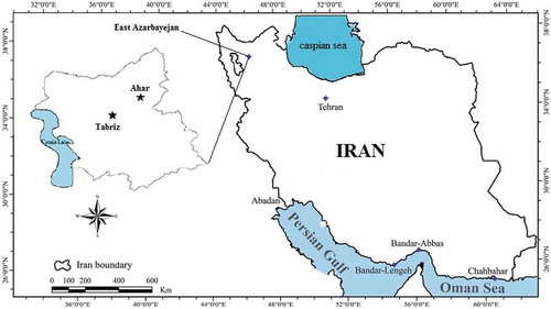
Ahar is one of the major cities of the East Azerbaijan province and the city center of Ahar in the north of the province. The area is about 13 km². The city of Ahar is located at an altitude of 1360 m above sea level. This city is located in a mountainous region. The average annual rainfall of Ahar is 350 mm. The maximum temperature of Ahar is 34°C and the minimum temperature below 0°C.

2.2. Soft computing techniques

2.2.1. GP regression

GP regression relies upon the postulation that nearby study must share the knowledge mutually and it is an approach of state of earlier straight over the function space. The generalization of Gaussian distribution is known as Gaussian regression. The matrix and vector of Gaussian distribution are articulated as covariance and mean in GP regression. Due to having earlier knowledge of functional dependence and data, the validation for generalization is not crucial. The GP regression models are capable to distinguish the forecast distribution consequent to the input test data (Rasmussen & Williams, 2006).

A GP is the choice of numbers of the random variable, any finite number of them has a collective multivariate Gaussian distribution. Assume p and q stand for input and target domain accordingly, thereupon x pairs (g_i, h_i) are drawn liberally and equivalently distribution. For regression, it is assumed that h ⊆ R_e then a GP on p is represented by the mean function $V_0:p\to Re$ and covariance function $\mu :p\times p\to Re$. Readers are requested to follow the Kuss (2006) to get the exhaustive details of GP. Pearson VII kernel function is used in this study

$\mathrm{P}\mathrm{e}\mathrm{a}\mathrm{r}\mathrm{s}\mathrm{o}\mathrm{n}\mathrm{V}\mathrm{I}\mathrm{I}\mathrm{f}\mathrm{u}\mathrm{n}\mathrm{c}\mathrm{t}\mathrm{i}\mathrm{o}\mathrm{n}\mathrm{k}\mathrm{e}\mathrm{r}\mathrm{n}\mathrm{e}\mathrm{l}\left(\mathrm{P}\mathrm{U}\mathrm{K}\right)=\left({1/\left[1+{\left(2{\sqrt{∥{\mathrm{x}}_{\mathrm{i}}-{\mathrm{x}}_{\mathrm{j}}∥}}^2\sqrt{2^{\left(1/\omega \right)}-1}/\sigma \right)}^2\right]}^{\omega }\right)$

Here Gaussian noise, $\sigma$ and $\omega$ are the kernel constraints of GP_PUK model.

2.3. M5P model (M5P)

M5P tree, first time introduced by Quinlan (1992), is used to develop a decision tree by engaging the linear regression function approach at nodes with an aim of constructing a model which proposes a correlation among the target value of the training cases and value of input attributes. The splitting approach is applied at each node instead to gain the maximum information to minimize the variation in the intra-subset class value down to each branch. The splitting process will be converged when there are diminutive variations among the class values of the instances or left only a few instances or when the tree is pruned back. The developed tree shows the very good structure and prediction accuracy due to showing more potential linearity at the leaf node.

2.4. Random forests

RF is a highly flexible assembly of decision trees that perform well for linear and nonlinear estimation by adjusting variance and bias (Breiman, 1996, 2001). This assembly learning process is identified as “bagging” as it develops trees in which consecutive trees do not base on former trees. Every tree is separately estimated using a bootstrap sample of the dataset and a simple commonly vote is considered for final estimation (Liaw & Wiener, 2002). RF model requires two specific standard parameters: quantity of input variables (m) implemented at every node to develop a tree and the number of trees to be developed (k). Thus, the RF regression contains k number of trees, which is searched through for the best split.

2.5. Multilayer perceptron

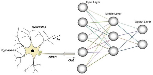
McCulloch and Pitts (1943) proposed ANN for the first time. In general, the layered perceptron neural network structure contains three layers: input, hidden, and the target layer. Each layer includes the number of neurons (Figure 2). The number of neurons in the input and output layers is determined by the nature of the problem under consideration, while the number of neurons in the hidden layers, as well as the number of these layers, is determined by the trial and errors to reduce the amount of error by the user (Firat & Gungor, 2009; Schalkoff, 1997). Each of the neurons in the input layer is weighted whose value determines the effect of each variable on the input layer performance. Each neuron consists of two parts: in the first part of it, the weighted sum of the input values is computed and in the second part of the neuron, the output of the first part is located in a mathematical function and through which the output of the neuron is calculated. This mathematical function is referred to as the actuator function, the threshold function, or the transfer function which functions as a nonlinear filter and makes the output of the neuron in a particular number range (Ghorbani, Khatibi, Goel, FazeliFard, & Azani, 2016).

Figure 2. Simple configuration of multilayer perceptron neural network.

2.6. Data analysis

The dataset contains ST and other meteorological parameters including variables such as air temperature, relative humidity, wind speed, sunshine hours, and ST at depths of 5 cm, which have been taken from Tabriz and Ahar meteorological station of Iran. Dataset used in this study was recorded between the years of 2013 and 2015. The average air temperature lies between the −13°C and 32.2°C in Tabriz and −13.5°C and 28.2°C in Ahar. The range of the ST at 5 cm depth lies between −8.13°C and 39°C in Tabriz and −5.27°C to 35.93°C in Ahar. Table 1 represents the features of the dataset used in this study. The data scale is the daily average. Table 2 represents the input variables and input combination that are considered for modeling. 75% of the total dataset was selected for the training the model and rest 25% was used for the testing the developed models.

Table 1. Statistical data of climate variables of Tabriz and Ahar stations.

Tabriz	Variables	Skewness	Stretch index	Average	Min	Max	Standard deviation
	Average air temperature (°C)	−0.21	−0.9	13.58	−13	32.2	10.26
	Sunny hours average (h)	−0.78	−0.45	8.01	0	13.5	3.74
	Average relative humidity (%)	0.23	−1.03	51.18	14.12	94.37	18.21
	Average wind speed (km·h^−1)	0.73	0.012	3.7	0	10.62	1.71
	Soil temperature at 5 cm depth (°C)	0.005	−1.31	17.42	−8.13	39	12.43
Ahar	Variables	Skewness	Stretch index	Average	Max	Min	Standard deviation
	Average air temperature (°C)	−0.29	−0.82	11.67	−13.5	28.2	8.62
	Sunny hours average (h)	−0.59	−0.77	7.42	0	13/6	3.91
	Average relative humidity (%)	0.28	−0.48	58.21	22.62	97	15.28
	Average wind speed (km·h^−1)	1.21	1.24	3.25	0	15.75	1.71
	Soil temperature at 5 cm depth (°C)	0.095	−1.36	14.88	−5.27	35.93	11.22

Table 2. Selecting different modes for modeling soil temperature estimates with a delay of 2 days for depth of 5 cm.

Structure	Entrance	Output
1	T(t − 2)	Soil temperature at a depth of 5 cm
2	T(t − 2) + RH(t − 2)	Soil temperature at a depth of 5 cm
3	T(t − 2) + RH(t − 2) + SUN(t − 2)	Soil temperature at a depth of 5 cm
4	T(t − 2) + RH(t − 2) + SUN(t − 2) + W(t − 2)	Soil temperature at a depth of 5 cm
5	T(t−2) + RH(t − 2) + W(t − 2)	Soil temperature at a depth of 5 cm

3. Models evaluation

After analyzing data with a variety of methods and models, their performance needs to be evaluated. There are various ways to do this. The most important of these methods is to compare the observational and computational values of models using evaluation criteria. In this study mean absolute error (MAE), root mean square error (RMSE), and the coefficient of determination (CC) are used to evaluate the performance of developed models and their relationships are given below. Lower values of RMSE, MAE and higherCC values indicate that developed model is more perfect (Sihag, Singh, SepahVand, & Mehdipour, 2018b), where m and n are observational and computational estimates of the ST at the time of i, a number of data

(1) $MAE=\frac{1}{a}(\sum _{i=1}^a\left|m-n\right|$(1)

(2) $RMSE=\sqrt{\frac{1}{a}(\sum _{i=1}^a{\left(m-n\right)}^2}$(2)

(3) $CC=\frac{a\sum mn-(\sum m)(\sum n)}{\sqrt{a(\sum m^2)-{(\sum m)}^2}\sqrt{a(\sum n^2)-{(\sum n)}^2}}$(3)

4. Result and discussion

4.1. Results of GP

The Pearson VII kernel function-based GP model was implemented using WEKA 3.9. The optimum values of GP_PUK models with Gaussian noise = 0.01, ω = 0.1, and σ = 1 are kept constant for all models for the fair comparison among models. Table 3 represents the results obtained (MAE, RMSE, and CC) by GP_PUK model for Tabriz and Ahar metrological stations respectively. These assessment criteria values shows that model GP_PUK4 (dependent variables of average air temperature, average sunny hours, average relative humidity, and average wind speed are provided in Table 2) performs relatively better than other models with testing MAE = 2.7741°C, RMSE = 3.4742°C, and CC = 0.9696 for Tabriz and MAE = 5.4103°C, RMSE = 6.6202°C, and CC = 0.8562 for Ahar stations.

Table 3. The results of modeling with Pearson VII kernel function-based GP models for Tabriz and Ahar at a depth of 5 cm.

Models	Tabriz
	Training			Testing
	MAE (°C)	RMSE (°C)	CC	MAE (°C)	RMSE (°C)	CC
GP_PUK1	2.4368	3.1289	0.9650	3.0404	3.9284	0.9586
GP_PUK2	0.0631	0.3228	0.9996	3.9947	5.1962	0.9270
GP_PUK3	0.0019	0.0032	1.0000	2.8156	3.5798	0.9666
GP_PUK4	0.0009	0.0012	1.0000	2.7741	3.4742	0.9696
GP_PUK5	0.0020	0.0047	1.0000	2.9947	3.7844	0.9622
	Ahar
GP_PUK1	4.5014	5.6524	0.8524	6.0310	7.3045	0.8195
GP_PUK2	0.1044	0.4931	0.9990	7.3778	9.2538	0.6973
GP_PUK3	0.0034	0.0094	1.0000	5.9536	7.3060	0.8074
GP_PUK4	0.0019	0.0048	1.0000	5.4103	6.6202	0.8562
GP_PUK5	0.0039	0.0084	1.0000	6.0319	7.6266	0.8024

Bold values indicate the best performing model.

Figures 3 and 4 present the detail of actual and estimated ST at 5 cm depth and their corresponding scatter plot for the best GP_PUK model using testing dataset for Tabriz and Ahar stations respectively. It is clearly noted from Table 3 and Figures 4 and 5 that GP-PUK4 model is suitable for estimating the ST of both stations.

Figure 3. Comparison of actual and predicted soil temperature at 5 cm and agreement diagram for Tabriz metrological station – Pearson VII kernel function-based GP model, testing period.

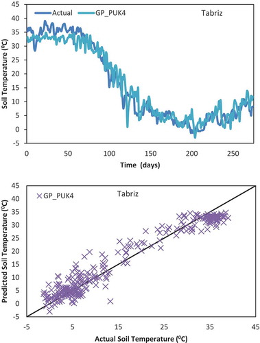
Figure 4. Comparison of actual and predicted soil temperature at 5 cm and agreement diagram for Ahar metrological station – Pearson VII kernel function-based GP model, testing period.

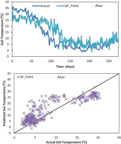
Figure 5. Comparison of actual and predicted soil temperature at 5 cm and agreement diagram for Tabriz metrological station – M5P model, testing period.

4.2. Results of the M5P model

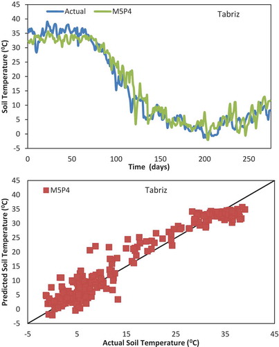
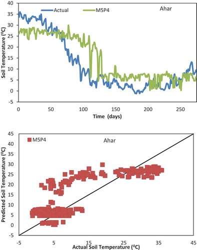
The M5P model was implemented using WEKA 3.9. The process of development of M5P model is same as GP_PUK model trial and error process Table 4 presents the results obtained (MAE, RMSE, and CC) by GP_PUK model for Tabriz and Ahar metrological stations respectively. These performance evaluation criteria values show that model M5P4 performs quite better than other models with testing MAE = 2.7106°C, RMSE = 3.4563°C, and CC = 0.9692 for Tabriz and MAE = 5.5907°C, RMSE = 6.9010°C, and CC = 0.8448 for Ahar stations.

Table 4. The results of modeling with M5P models for Tabriz and Ahar at a depth of 5 cm.

Models	Tabriz
	Training			Testing
	MAE (°C)	RMSE (°C)	CC	MAE (°C)	RMSE (°C)	CC
M5P1	2.7371	3.4992	0.9560	2.6340	3.2935	0.9728
M5P2	2.5042	3.2365	0.9625	2.7241	3.4834	0.9684
M5P3	2.4425	3.1665	0.9641	2.7697	3.5270	0.9679
M5P4	2.3647	3.1031	0.9655	2.7106	3.4563	0.9692
M5P5	2.4473	3.1962	0.9634	2.6871	3.4235	0.9696
	Ahar
M5P1	5.0539	6.2918	0.8131	5.3557	6.6469	0.8535
M5P2	4.9483	6.0115	0.8311	5.6708	7.0755	0.8354
M5P3	4.5374	5.6238	0.8541	5.5610	7.0044	0.8299
M5P4	4.7013	5.7717	0.8456	5.5907	6.9010	0.8448
M5P5	4.8876	5.9343	0.8358	5.7101	7.1277	0.8320

Bold values indicate the best performing model.

Figures 5 and 6 display the detail of actual and estimated ST at 5 cm depth and their corresponding scatter plot for the best M5P model using testing dataset for Tabriz and Ahar stations respectively. It is clearly noted from Table 4 and Figures 5 and 6 that M5P4 model is suitable than other models for estimating the ST of both Tabriz and Ahar stations.

Figure 6. Comparison of actual and predicted soil temperature at 5 cm and agreement diagram for Ahar metrological station – M5P model, testing period.

4.3. Results of the RF model

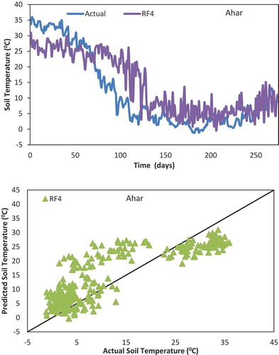
The RF model is developed as GP_PUK and M5P models. In this study, the RF model with parameters (k = 1, m = 1, I = 100) was used for ST modeling; the accuracy of RF models depends on these parameters. The results of the RF model for every data model definitions (see Table 2) are listed in Table 5 in terms of MAE, RMSE, and CC. The assessment criteria indicate that the RF4 model (dependent variables of T(t − 2), RH(t − 2), SUN(t − 2), W(t − 2), see Table 2) is suitable and works better than the other models for both Tabriz and Ahar stations.

Table 5. The results of modeling with RF models for Tabriz and Ahar at a depth of 5 cm.

Models	Tabriz
	Training			Testing
	MAE (°C)	RMSE (°C)	CC	MAE (°C)	RMSE (°C)	CC
RF1	2.1748	2.8435	0.9712	2.9012	3.7893	0.9633
RF2	1.0435	1.3652	0.9936	2.9360	3.8205	0.9624
RF3	1.0221	1.3259	0.9942	2.7948	3.5322	0.9690
RF4	1.0230	1.3335	0.9943	2.8455	3.4722	0.9728
RF5	1.0157	1.3195	0.9943	2.7874	3.5619	0.9690
	Ahar
RF1	4.0636	5.2105	0.8762	6.3293	7.8062	0.7926
RF2	2.0039	2.5155	0.9753	6.2698	7.6817	0.7950
RF3	1.7278	2.2008	0.9817	5.7205	6.9710	0.8324
RF4	1.6979	2.1423	0.9835	5.5501	6.8549	0.8436
RF5	1.8673	2.3385	0.9799	5.8844	7.3743	0.8193

Bold values indicate the best performing model.

Figure 7 and 8 display the detail of actual and predicted ST at 5 cm depth and their corresponding scatter plot for the best RF model using the testing dataset for Tabriz and Ahar stations respectively. It is clearly noted from Table 5 and Figures 7 and 8 that the RF model is suitable for estimating the ST of both Tabriz and Ahar stations. The results show further improvements in the prediction of ST in terms of reduced scatter. In particular, there is variation in the predicted peak values compared with the actual values for both stations.

Figure 7. Comparison of actual and predicted soil temperature at 5 cm and agreement diagram for Tabriz metrological station – RF model, testing period.

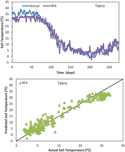
Figure 8. Comparison of actual and predicted soil temperature at 5 cm and agreement diagram for Ahar metrological station – RF model, testing period.

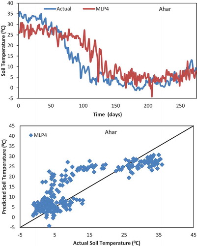
Results of MLP: The MLP modeling was implemented using WEKA 3.9 software. In this study, single hidden layer is used for developing models with learning rate 0.2, momentum 0.1, and iteration 1500. The optimum number of neurons was identified using trial and error method by changing the number of neurons in the hidden layer from 1 to 25. The optimum number of the neurons in the hidden layer for each combination is listed in Table 6. The performance of MLP-based models for Tabriz and Ahar stations is listed in Table 7 in terms of MAE, RMSE, and CC. These performance evaluation criteria values show that model MLP4 (4-13-1) performs quite better than other models with testing MAE = 2.5525°C, RMSE = 3.2626°C, and CC = 0.9718 for Tabriz and MLP4 (4-9-1) model with MAE = 5.1261°C, RMSE = 6.3332°C and CC = 0.8619 for Ahar stations.

Table 6. Structure of the MLP-based model.

Models	Tabriz
	Structure of the MLP
MLP1	1-8-1
MLP2	2-1-1
MLP3	3-1-1
MLP4	4-13-1
MLP5	3-5-1
	Ahar
MLP1	1-25-1
MLP2	2-8-1
MLP3	3-14-1
MLP4	4-9-1
MLP5	3-23-1

Table 7. The results of modeling with MLP models for Tabriz and Ahar at a depth of 5 cm.

Models	Tabriz
	Training			Testing
	MAE (°C)	RMSE (°C)	CC	MAE (°C)	RMSE (°C)	CC
MLP1	2.7504	3.4995	0.9560	2.6422	3.2876	0.9729
MLP2	2.7602	3.5385	0.9550	2.6912	3.4151	0.9703
MLP3	2.7237	3.5218	0.9569	2.5965	3.2724	0.9728
MLP4	2.3703	3.0819	0.9664	2.5525	3.2626	0.9718
MLP5	2.6849	3.4821	0.9564	2.5862	3.3040	0.9719
	Ahar
MLP1	5.2196	6.3906	0.8098	5.2436	6.3446	0.8653
MLP2	5.1136	6.1346	0.8275	5.3283	6.4985	0.8532
MLP3	4.5904	5.6653	0.8518	5.2046	6.3427	0.8618
MLP4	4.4826	5.5747	0.8570	5.1261	6.3332	0.8619
MLP5	4.7300	5.8143	0.8431	5.2867	6.7915	0.8521

Bold values indicate the best performing model.

Figure 9 and 10 display the detail of actual and predicted ST at 5 cm depth and their corresponding scatter plot for the best MLP model using the testing dataset for Tabriz and Ahar stations respectively. It is clearly noted from Table 7 and Figures 9 and 10 that MLP4 model is suitable for estimating the ST of both Tabriz and Ahar stations.

Figure 9. Comparison of actual and predicted soil temperature at 5 cm and agreement diagram for Tabriz metrological station – MLP model, testing period.

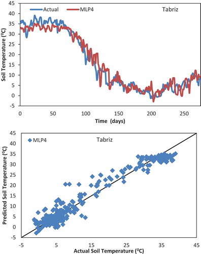
Figure 10. Comparison of actual and predicted soil temperature at 5 cm and agreement diagram for Ahar metrological station – MLP model, testing period.

5. Discussion

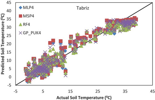
This section presents the comparison of prediction ability of MLP-, GP-, M5P-, and RF-based models. The comparison of the best-selected model among all the four techniques was done by using the standard statistical performance evaluation parameters (MAE, RMSE, and CC).

The details of the best-selected models with MLP, GP, M5P, and RF are listed in Table 8 and Figure 11 for Tabriz station. Table 8 and Figure 11 suggest that MLP4 models work better than GP_PUK-, M5P-, and RF-based models. Model 4 (dependent variables of average air temperature, average sunny hours, average relative humidity, and average wind speed (Table 2)) performs better than other combinations. In Figure 11, predicted values of the ST at 5 cm are closer to the line of the perfect agreement for Tabriz station.

Table 8. The results of different modeling approaches for Tabriz at a depth of 5 cm.

Models	Tabriz
	Training			Testing
	MAE (°C)	RMSE (°C)	CC	MAE (°C)	RMSE (°C)	CC
GP_PUK4	0.0009	0.0012	1.0000	2.7741	3.4742	0.9696
M5P4	2.3647	3.1031	0.9655	2.7106	3.4563	0.9692
RF4	1.0230	1.3335	0.9943	2.8455	3.4722	0.9728
MLP4	2.3703	3.0819	0.9664	2.5525	3.2626	0.9718

Bold values indicate the best performing model.

Figure 11. Agreement plot of actual and predicted values of soil temperature at 5 cm for Tabriz metrological station – using MLP, M5P, RF, and GP-based models model, testing period.

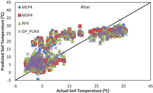
Table 9 and Figure 12 suggest that MLP4 models work better than GP_PUK-, M5P-, and RF-based models. Model 4 (dependent variables of average air temperature, average sunny hours, average relative humidity, and average wind speed (Table 2)) performs better than other combinations. In Figure 12, predicted values of the ST at 5 cm are closer to the line of the perfect agreement for Ahar station.

Table 9. The results of different modeling approaches for Ahar at a depth of 5 cm.

Models	Ahar
	Training			Testing
	MAE (°C)	RMSE (°C)	CC	MAE (°C)	RMSE (°C)	CC
GP_PUK4	0.0019	0.0048	1.0000	5.4103	6.6202	0.8562
M5P4	4.7013	5.7717	0.8456	5.5907	6.9010	0.8448
RF4	1.6979	2.1423	0.9835	5.5501	6.8549	0.8436
MLP4	4.4826	5.5747	0.8570	5.1261	6.3332	0.8619

Bold values indicate the best performing model.

Figure 12. Agreement plot of actual and predicted values of soil temperature at 5 cm for Ahar metrological station – using MLP, M5P, RF, and GP-based models model, testing period.

Öztürk et al. (2011) developed ANN-based models for forecasting the STs using eight different variables, which are latitude, longitude, altitude, month number, solar radiation, sunshine duration, temperature, and year. It was concluded that the estimated values using the ANN-based model lie very close to actual values for all depths. Numerous researchers implemented latitude, longitude, and altitude to estimate solar radiation (Citakoglu, 2015; Mohandes, Rehman, & Halawani, 1998; Siqueira, Tiba, & Fraidenraich, 2010). Tabari, Somee, and Zadeh (2011) used precipitation, relative humidity, air temperature, and solar radiation data of MLR- and ANN-based models to estimate STs at various soil depths and reported that ANN is more appropriate than MLR. In the present research, ST was estimated with average air temperature, sunshine hours, average relative humidity, and average wind using MLP, GP, RF, and M5P models and results of this study indicate that MLP works better than other techniques. Kisi et al. (2015) used only Mersin station to estimate STs and found that air temperature is the most important variable in modeling ST for Mersin, Turkey.

6. Conclusion

In this study, the Pearson VII kernel function-based GP, M5P, RF, and MLP models were used to estimate the DST. In this regard, different input structures (Table 2) were used. Finally, the accuracy of each model and the accuracy of each structure in ST estimation were investigated. The statistical period of the data was 3 years. Comparison of the performance of these models in estimating ST showed that MLP4 with much higher accuracy and less error than other models estimates the ST. MLP4 model includes the combination of average air temperature, average sunny hours, average relative humidity, and average wind speed which shows superior performance than other input combination-based models with all approaches.

Due to the better performance of the MLP model for DST modeling in East Azerbaijan province of Iran, it is recommended to use the MLP model at other stations. Also, this model could be used in other time-dependent applications based on the availability of different parameters.

Disclosure statement

No potential conflict of interest was reported by the authors.

References

- Atluri, V., Hung, C. C., & Coleman, T. L. (1999). An artificial neural network for classifying and predicting soil moisture and temperature using Levenberg-Marquardt algorithm. In Proceedings IEEE Southeastcon'99. Technology on the Brink of 2000 (Cat. No.99CH36300) (pp. 10–13). Lexington, KY: IEEE.
- Bilgili, M. (2010). Prediction of soil temperature using regression and artificial neural network models. Meteorology and Atmospheric Physics, 110(1–2), 59–70.
- Breiman, L. (1996). Bagging predictors. Machine Learning, 24(2), 123–140.
- Breiman, L. (2001). Random forests. Machine Learning, 45(1), 5–32.
- Citakoglu, H. (2015). Comparison of artificial intelligence techniques via empirical equations for prediction of solar radiation. Computers and Electronics in Agriculture, 118, 28–37.
- Citakoglu, H. (2017). Comparison of artificial intelligence techniques for prediction of soil temperatures in Turkey. Theoretical and Applied Climatology, 130(1–2), 545–556.
- Firat, M., & Gungor, M. (2009). Generalized regression neural networks and feed forward neural networks for prediction of scour depth around bridge piers. Advances in Engineering Software, 40(8), 731–737.
- Ghorbani, M. A., Khatibi, R., Goel, A., FazeliFard, M. H., & Azani, A. (2016). Modeling river discharge time series using support vector machine and artificial neural networks. Environmental Earth Sciences, 75(8), 685.
- Hillel, D. (1998). Environmental Soil Physics (pp. 771). San Diego,CA: Academic Press.
- Kang, S., Kim, S., Oh, S., & Lee, D. (2000). Predicting spatial and temporal patterns of soil temperature based on topography, surface cover, and air temperature. Forest Ecology and Management, 136(1–3), 173–184.
- Kätterer, T., & Andrén, O. (2009). Predicting daily soil temperature profiles in arable soils in cold temperate regions from air temperature and leaf area index. ActaAgriculturaeScandinavica Section B–Soil and Plant Science, 59(1), 77–86.
- Kim, S., & Singh, V. P. (2014). Modeling daily soil temperature using data-driven models and spatial distribution. Theoretical and Applied Climatology, 118(3), 465–479.
- Kisi, O., Sanikhani, H., & Cobaner, M. (2017). Soil temperature modeling at different depths using neuro-fuzzy, neural network, and genetic programming techniques. Theoretical and Applied Climatology, 129(3–4), 833–848.
- Kisi, O., Tombul, M., & Kermani, M. Z. (2015). Modeling soil temperatures at different depths by using three different neural computing techniques. Theoretical and Applied Climatology, 121(1–2), 377–387.
- Kuss, M., 2006. Gaussian process models for robust regression, classification, and reinforcement learning ( Doctoral dissertation, TechnischeUniversität).
- Liaw, A., & Wiener, M. (2002). Classification and regression by randomForest. R News, 2(3), 18–22.
- McCulloch, W. S., & Pitts, W. (1943). A logical calculus of the ideas immanent in nervous activity. The Bulletin of Mathematical Biophysics, 5(4), 115–133.
- Mehdipour, V., & Memarianfard, M. (2017a). Application of Support Vector Machine and Gene Expression Programming on Tropospheric ozone Prognosticating for Tehran Metropolitan. Civil Engineering Journal, 3(8), 557–567.
- Mehdipour, V., Memarianfard, M., & Homayounfar, F. (2017). Application of Gene Expression Programming to water dissolved oxygen concentration prediction. International Journal of Human Capital in Urban Management, 2(1), 39–48.
- Mehdipour, V., & Memarianfardb, M. (2017b). Civil Engineering Journal. Civil Engineering, 3(8), 557–567.
- Mehdizadeh, S., Behmanesh, J., & Khalili, K. (2017). Evaluating the performance of artificial intelligence methods for estimation of monthly mean soil temperature without using meteorological data. Environmental Earth Sciences, 76(8), 325.
- Miles, A., & Brown, M. (2007). Teaching Organic Farming and Gardening: Resources for Instructors. Santa Cruz: University of California Farm and Garden.
- Mohandes, M., Rehman, S., & Halawani, T. O. (1998). Estimation of global solar radiation using artificial neural networks. Renewable Energy, 14(1–4), 179–184.
- Nahvi, B., Habibi, J., Mohammadi, K., Shamshirband, S., & Al Razgan, O. S. (2016). Using self-adaptive evolutionary algorithm to improve the performance of an extreme learning machine for estimating soil temperature. Computers and Electronics in Agriculture, 124, 150–160.
- Öztürk, E., Atsan, E., Polat, T., & Kara, K. (2011). Variation in heavy metal concentrations of potato (Solanumtuberosum L.) cultivars. Journal of Animal Plant Science, 21(2), 235–239.
- Parsaie, A., & Haghiabi, A. H. (2015). Predicting the longitudinal dispersion coefficient by radial basis function neural network. Modeling Earth Systems and Environment, 1(4), 34.
- Parsaie, A., Yonesi, H. A., & Najafian, S. (2015). Predictive modeling of discharge in compound open channel by support vector machine technique. Modeling Earth Systems and Environment, 1(1–2), 1.
- Quinlan, J. R., 1992, November. Learning with continuous classes. In 5th Australian joint conference on artificial intelligence (Vol.92, pp. 343–348). Singapore: World Scientific.
- Rasmussen, C. E., & Williams, C. K. (2006). Gaussian process for machine learning. Cambridge, England: MIT Press.
- Schaetzl, R. J., Knapp, B. D., & Isard, S. A. (2005). Modeling soil temperatures and the mesic-frigid boundary in the central Great Lakes region, 1951–2000. Soil Science Society of America Journal, 69(6), 2033–2040.
- Schalkoff, R. J. (1997). Artificial neural networks (Vol. 1). New York: McGraw-Hill.
- Shiri, J., & KişI, Ö. (2011). Comparison of genetic programming with neuro-fuzzy systems for predicting short-term water table depth fluctuations. Computers & Geosciences, 37(10), 1692–1701.
- Sihag, P. (2018). Prediction of unsaturated hydraulic conductivity using fuzzy logic and artificial neural network. Modeling Earth Systems and Environment, 4(1), 189–198.
- Sihag, P., Singh, B., SepahVand, A., & Mehdipour, V. (2018b). Modeling the infiltration process with soft computing techniques. ISH Journal of Hydraulic Engineering, 1–15. doi:10.1080/09715010.2018.1464408
- Sihag, P., Tiwari, N. K., & Ranjan, S. (2017). Prediction of unsaturated hydraulic conductivity using adaptive neuro-fuzzy inference system (ANFIS). ISH Journal of Hydraulic Engineering, 1–11. doi:10.1080/09715010.2017.1381861
- Sihag, P., Tiwari, N. K., & Ranjan, S. (2018a). Support vector regression-based modeling of cumulative infiltration of sandy soil. ISH Journal of Hydraulic Engineering, 1–7. doi:10.1080/09715010.2018.1439776
- Singh, B., Sihag, P., & Singh, K. (2017). Modelling of impact of water quality on infiltration rate of soil by random forest regression. Modeling Earth Systems and Environment, 3(3), 999–1004.
- Singh, R. B. (2000). Environmental consequences of agricultural development: A case study from the Green Revolution state of Haryana, India. Agriculture, Ecosystems & Environment, 82(1–3), 97–103.
- Siqueira, A. N., Tiba, C., & Fraidenraich, N. (2010). Generation of daily solar irradiation by means of artificial neural net works. Renewable Energy, 35(11), 2406–2414.
- Sun, B., Zhang, L., Yang, L., Zhang, F., Norse, D., & Zhu, Z. (2012). Agricultural non-point source pollution in China: Causes and mitigation measures. Ambio, 41(4), 370–379.
- Tabari, H., Somee, B. S., & Zadeh, M. R. (2011). Testing for long-term trends in climatic variables in Iran. Atmospheric Research, 100(1), 132–140.
- Talaee, P. H. (2014). Daily soil temperature modeling using neuro-fuzzy approach. Theoretical and Applied Climatology, 118(3), 481–489.
- Tiwari, N. K., Sihag, P., Kumar, S., & Ranjan, S. (2018). Prediction of trapping efficiency of vortex tube ejector. ISH Journal of Hydraulic Engineering, 1–9. doi:10.1080/09715010.2018.1441752
- Wu, W., Tang, X. P., Guo, N. J., Yang, C., Liu, H. B., & Shang, Y. F. (2013). Spatiotemporal modeling of monthly soil temperature using artificial neural networks. Theoretical and Applied Climatology, 113(3–4), 481–494.