Demography of the bottlenose dolphin Tursiops truncatus (Mammalia: Delphinidae) in the Eastern Ligurian Sea (NW Mediterranean): quantification of female reproductive parameters

Abstract

The reproductive histories of 41 adult bottlenose dolphin females were analysed using photo-identification data collected between 2006 and 2014 in four sub-areas of the eastern Ligurian Sea (northwest Mediterranean). The Rapallo sub-area revealed the highest (highly significant) frequency of encounters (per unit effort) of reproductive females in association with young individuals, therefore emerging as a candidate nursery area in the region. The estimated fertility rate of adult females ranged between 290 and 407 births per 1000 individuals per year, higher than that of other known bottlenose dolphin populations, with a calving interval between 2.45 and 3.5 years. These results will be useful for projecting future trends of this (sub)population.

Keywords:

• Marine mammal population reproductive output
• fertility rate
• cub mortality
• calving interval
• individual life history

Introduction

When variation in male abundance does not limit female reproduction (as for polygamous or promiscuous species), knowledge of female reproduction parameters is key to assessing population viability and formulating conservation plans (Caswell 2001; Fujiwara & Caswell 2001).

Understanding the life history of long-lived species requires detailed information on fertility and mortality parameters (Caswell 2001; Stanton & Mann 2012). A first approach to investigating cetaceans’ life histories has been based on stranding data (Stolen & Barlow 2003; Arrigoni et al. 2011). Another fruitful approach is based on data sets of sightings (possibly repeated over a number of years) of individuals permanently marked by photo-identification techniques (Würsig & Jefferson 1990). These data, typically documenting nursery areas, group composition, social behaviour, spatial patterns and female reproduction, may provide valuable information on the population structure (Fujiwara & Caswell 2001; Rossi et al. 2014b; Fruet et al. 2015).

Although population studies are fundamental for conservation, little demographic knowledge is available for Mediterranean cetaceans (Rossi et al. 2014b). So far the only available demographic studies regard the population structure of the Mediterranean fin whale (Balaenoptera physalus), analysed by both stranding (Arrigoni et al. 2011) and photo-identification data (Rossi et al. 2014b), and the mortality of the Mediterranean bottlenose dolphin analysed by strandings along Italian and French Mediterranean coasts (Rossi et al. 2014a).

Exhibiting a cosmopolitan distribution, since it has adapted to a large variety of environmental conditions, the bottlenose dolphin Tursiops truncatus (Montagu, 1821) is one of the most studied cetaceans worldwide (Wells & Scott 2009; and references therein; Gnone et al. 2011). This species’ distribution is primarily shallow water (< 100–200 m) in coastal or continental shelf habitat, though it is also found in pelagic waters (Wells & Scott 2009). In the Mediterranean, the bottlenose dolphin inhabits shallow coastal waters, especially in the northwest (Gnone et al. 2011). This exposes bottlenose dolphins to a number of direct and indirect anthropogenic threats, such as chemical and acoustic pollution, environmental degradation, overfishing, epizootic outbreaks and disturbance from boating (Bearzi et al. 2008). Since 2009 the Mediterranean population has been judged vulnerable by the International Union for Conservation of Nature (IUCN; Bearzi & Fortuna 2006).

In the present paper a 9-year photo-identification data set of bottlenose dolphin based on sightings from the eastern Ligurian Sea was analysed with the purpose to identify nursery areas and to estimate the fertility rate, the calving interval and mortality during the first year of life in this area.

Materials and methods

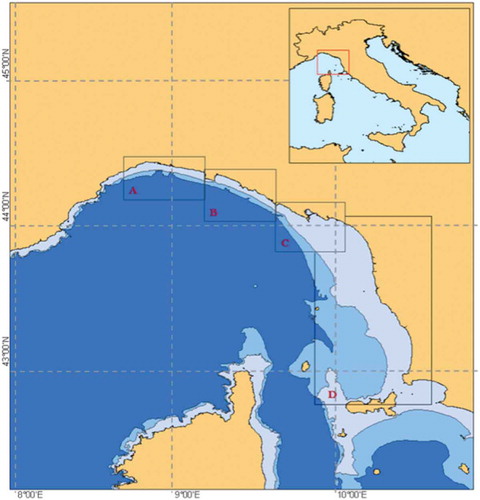
Data were collected between January 2006 and October 2014 by the research groups “Delfini Metropolitani” (Acquario di Genova) and CE.TU.S. (CEntro TUrsiopi e Stenelle), in the eastern Ligurian Sea (North Western Mediterranean) within a general study aiming to investigate the spatial distribution and abundance, and the spatial mobility, of bottlenose dolphin in the study area. The study area was divided into the following four sub-areas: A, Capo Arenzano–Punta Chiappa; B, Punta Chiappa–Punta Mesco; C, Punta Mesco–Punta Bianca; D, Punta Bianca–northern Elba Island (Figure 1), mainly based on the underlying homogeneity in the geo-morphological traits of the coastal strip. Sub-area A is characterised by rocky shores and a narrow continental shelf (the 200-m isobath running around 4–8 km from the coast line), and by two deep marine canyons, crossing the area in front of Genoa; this sub-area is affected by a strong anthropogenic impact, due to the proximity of Genoa harbour, with its intense maritime traffic. Sub-area B has geomorphological traits resembling those of sub-area A, with a narrow, rocky continental shelf, but is affected by a lower human activity, especially in its poorly anthropised eastern part. Sub-area C has geomorphological traits, which are transitional between sub-area B and sub-area D; the continental shelf starts to enlarge (the 200-m isobath runs over 30 km from the coast line) and the bottom is mainly covered by fine debris (mud), due to the terrestrial runoff from the Magra River. Finally, sub-area D is characterised by a larger continental shelf (the 200-m isobath running 30–60 km from the coast line) presenting typical sandy/muddy and rocky communities.

Figure 1. The Eastern Ligurian Sea study area was divided into four sub-areas: A, Capo Arenzano–Punta Chiappa; B, Punta Chiappa–Punta Mesco; C, Punta Mesco–Punta Bianca; D, Punta Bianca–northern Elba Island.

Sighting surveys were carried out on random tracks throughout the year when sea conditions permitted (below Beaufort 4), using a 5.10-m inflatable boat and 12-m motor sailor catamaran. Photographic data were collected by digital reflex camera. Effort tracks were recorded by GPS (Global Positioning System); a GIS (Geographic Information System) (ArcGIS, ESRI 2007) system was used to quantify the research effort (RE), measured in km of active observation under adequate weather conditions in the study areas.

During surveys multiple images were collected, and subsequently graded (up to final selection) based on the quality of the image, and the distinctiveness of the animals (Gnone et al. 2011). Quality assessment was based on visibility of the fin, focus, lighting, angle of the fin with respect to the photographer, and contrast between dorsal fin and background, which are well-acknowledged criteria in the literature (Whitehead et al. 1997; Read et al. 2003). Distinctiveness was based on the presence of natural marks on the dorsal fin. In particular, notches, deformities and unusual shapes of the dorsal fin were considered to be permanent marks and used as primary distinctive elements for the photo-identification of the animal. On the other hand, scars and discolourations were only used in association with primary distinctive elements to confirm identification (Würsig & Jefferson 1990; Gnone et al. 2011).

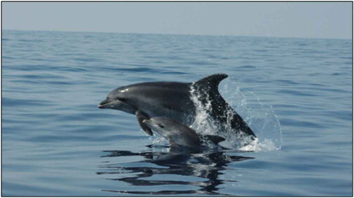
Each sighted bottlenose dolphin was assigned to one of the following life-stages: cub (< 180 cm, < 1 yr); calf (≥ 180 < 220 cm, ≥1 < 3 yr); juvenile (≥ 220 < 270 cm, ≥ 3 < 7 yr); adult: (≥ 270 cm, ≥ 7 yr) (Rossi et al. 2014a). Assignment to the appropriate stage was performed through a combination of criteria including the analysis of the selected images, behaviour observed in the field, and available information on life history for already sighted individuals. Only well-marked dolphins that could be consistently identified over a long-term period were considered adults. The young were tracked by following their well-marked (putative) mothers until weaning, since dolphins generally do not exhibit long-lasting marks on the dorsal fin during the first few years of life (Würsig & Jefferson 1990; Fruet et al. 2015). To categorise immature dolphins, the body size of the young was compared to that of the associated female. Temporary marks and specific behaviours, e.g. sharp dorso-ventral fetal folds and infant position, were used for cubs (Mann & Smuts 1998) (Figure 2). Further details are reported in the Appendix.

Figure 2. Mother–calf association (Photo credit: Alessia Rossi).

Sex determination was done both directly, by analysing the genital slits in the ventral region from photos taken during dolphins’ jumps or belly-up swimming, and indirectly (for reproductive females only) by observing prolonged associations between the same photo-identified adult individual with a young one (i.e. newborn, cub, or calf) throughout repeated sightings (and related photographic data) over time (Mann et al. 2000; Grellier et al. 2003).

The collected data were organised in the form of a sighting-reproduction history, reporting the sighting history of each well identified adult female individual (i.e. the sequence of dates when she was sighted in the surveyed period), jointly with information on whether she was sighted alone or in association with a young individual (cub, calf or juvenile).

The frequency of bottlenose dolphins in each sub-area A, B, C, D was evaluated by the encounter rate (ER), defined as the number of sighting events per km of research effort. The ER of females with cubs was calculated to check for the presence of possible nursing areas. Spatial variation in ERs between sub-areas was assessed by the standard bilateral test for the difference between Poisson rates, under the null hypothesis: H0 = “the ER is the same in each sub-area considered”. Briefly, assuming that sightings cumulate over the cumulated effort in a Poisson-like fashion, that is independently and with a constant small sighting probability per km of sighting effort, the number of observed sightings per each sub-area was compared with the 95% Poisson confidence region corresponding to the null hypothesis under the same total effort.

The fertility rate of adult bottlenose dolphin females, b, was estimated on the explicit assumption that fertility is independent of age, by making use of the nature of the data as a reproduction-history (see the Appendix). This allowed us to apply the classical definition of occurrence-exposure rate (Caswell 2001; Preston et al. 2006), by dividing the total number of young individuals observed in steady association with their mother by the total time that observed female individuals spent in exposure to the risk of childbearing. The latter was computed as the sum, throughout all adult females, of the individuals’ exposure times. Non-parametric 95% bootstrap confidence intervals are also computed. Details are reported in the Appendix.

The calving interval, i.e. the time between two consecutive births, was estimated two ways: (a) indirectly, from the estimated birth rate b, based on the assumption that new births to a mother add up regularly (in a Poisson-like fashion) at a time distance given by 1/b; and (b) directly, for females with at least two consecutive births in the study period (Tezanos-Pinto et al. 2015), as the average time distance between a female-with-cub sighting and a female-with-new cub sighting.

A cub is presumed to be dead if the mother is steadily sighted alone within 12 months since the first mother–cub sighting (Wells & Scott 1990; Mann et al. 2000; Tezanos-Pinto et al. 2015). A simple cub mortality was calculated by dividing the number of cubs that presumably died in their first year of life by the total number of cubs previously sighted with their (identified) mothers (Tezanos-Pinto et al. 2015).

Results

Overall, 37,477 km were covered throughout the entire area; a total of 286 adult dolphins were photo-identified, of which 41 fulfilled the strict requirements of the study design to be identified as reproductive females.

Field results are summarised in Table I, reporting, per each sub-area, the number of sightings of identified adult females and of identified adult females in association with a cub, respectively, the sighting effort (in km), and the resulting ER per 1000 km of sighting effort. The ER of identified adult females varied across sub-areas by a factor of 10, ranging between less than 2 (sub-area A) and 22 sightings per 1000 km (sub-area C), with an average ER of about 11 throughout the entire study area. The ER of females in association with a cub ranged between 0.25 (sub area A) and about 5.2 sightings per 1000 km (sub area B), with an average ER of 2.91 throughout the entire study area. The Poisson test for the equality of the ER of females with cubs throughout the four sub-areas indicates that the null hypothesis is always rejected at the nominal significance level of 0.05, suggesting that the difference between observed and expected sightings is always statistically significant. In particular, sub-area B, showing an observed number of sightings almost double the expectation under H₀ (p-value = 0.00006), emerges as a candidate nursing area.

Table I. Column 1 (from left): the surveyed sub-areas; column 2: observed number of sightings of females in association with young; in parentheses the corresponding expected number of sightings under hypothesis H₀ that the encounter rate (ER) is the same throughout the entire study area; column 3: total number of sightings of females alone or in association with young; in parentheses the corresponding expected number of sightings under the same H₀ hypothesis; column 4: sighting effort in km; column 5: ER of adult females in steady association with a young individual per 1000 km of sighting effort; column 6: ER of adult females, per 1000 km of sighting effort.

Sub-area	No. sightings of females with a young individual	No. of sightings of females	Sighting effort (km)	ER Female + cubs	ER All adults
A	1 (11.7, p = 0.00013)	7 (44.3)	4029.24	0.25	1.74
B	51 (28.7, p = 0.00006)	182 (108.7)	9883.91	5.16	18.41
C	25 (17.7, p = 0.0382)	132 (67.0)	6090.72	4.10	21.67
D	32 (50.8, p = 0.032)	91 (192.1)	17,473.28	1.83	5.21
Total	109	412	37,477.2	2.91	10.99

The analysis of the sighting-reproduction histories showed that the aforementioned 41 reproductive females were observed over years in steady association with 72 young individuals, of which 61 were cubs. The fertility rate of adult females is estimated (Table II) under four different scenarios (S1, S2, S3, S4) having the purpose to crudely handle the uncertainty embedded in the observation process. The first scenario (S1, taken as the baseline) posits that only the young individuals (cubs, calves, juveniles) observed in steady association with each sighted adult female actually represent births for that female. Scenario S2 (85 births) was created from scenario 1 by keeping fixed the female exposure time and imputing further births to account for those cases where two subsequent sightings of young individuals with the same mother were so distant in time to be consistent with at least an intermediate (unobserved) birth. Concretely, consider the case of a mother observed in steady association with a cub during a certain year, and re-sighted after 5 years in association with a new cub. Under the baseline scenario S1 two births were counted from this history, while in scenario S2 one further birth was considered, counting in total three births from that mother during that period. Finally, scenarios S3 and S4 were created in analogy to S1 and S2 by using only sightings of cubs (61 under S3 and 72 under S4, respectively) instead of sightings of all young individuals.

Table II. Female fertility under the four different scenarios described in the text. Per each scenario: (a) the number of births (first row); (b) the exposure time (second row); (c) the resulting fertility rate b (third row) per 1000 adult females yr⁻¹ (computed by dividing the number of births by the exposure time), in parentheses below, the corresponding 95% bootstrap percentile confidence interval (CI); (d) the corresponding predicted interval between births, computed as 1/b (fourth column).

	Scenario 1	Scenario 2	Scenario 3	Scenario 4
Number of births	74	85	61	72
Exposure time (yr)	255.5	255.5	176.8	176.8
Fertility rate b (per 1000 yr^−1)	289.6	332.7	344.9	407.1
	(CI: 259.5–321.3)	(CI: 296.6–372.3)	(CI: 311.9 – 379.6)	(CI: 371.4–443.9)
Births interval (yr)	3.45	3.0	2.90	2.45

The resulting fertility rate b ranges between a minimum of about 290 births per 1000 mothers yr⁻¹ (scenario 1) and a maximum of 407 births per 1000 mothers yr⁻¹ (scenario 4; see Table II, third row). The corresponding birth interval (or calving interval), estimated as 1/b, declines from 3.5 yr in scenario 1 up to 2.45 yr in scenario 4, respectively. These estimates bound well the estimate of the calving interval of 3.15 yr calculated directly by using the subset of females (22 individuals) that gave birth at least twice during the sighting period.

A cub is considered dead if the mother is steadily sighted alone within 12 months after the first mother-cub sighting (e.g. Wells & Scott 1990; Mann et al. 2000; Tezanos-Pinto et al. 2015). Since 44 mothers were re-sighted during the year following their first sighting with a cub, of which only 33 were still in steady association with a young individual, the number of dead cubs was 11 and the estimated cub mortality was 25% (11/44), corresponding to a cub survival of 75% (Table III).

Table III. Summary reproduction parameters of genus Tursiops in the literature. ^aThis study; ^bMitchenson (2008); ^cFruet et al. (2015); ^dWells and Scott (1990); ^eTezanos-Pinto et al. (2015); ^fHenderson et al. (2014); ^gKogi et al. (2004); ^hMann et al. (2000); ⁱSteiner and Bossley (2008).

Site	Species	Fertility rate (yr^−1)	Calving interval (yr)	Cub mortality rate
Eastern Ligurian Sea^a	T. truncatus	0.29–0.41	2.45–3.45	0.25
Scotland^b	T. truncatus	0.11	3.18	-
PLE, Brazil^c	T. truncatus	0.11	3	0.16
Sarasota Bay, USA^d	T. truncatus	0.144	4	0.19
Bay of Island, NZ^e	T. truncatus	0.25	4.3	0.34–0.52
Doubtful Sound, NZ^f	T. truncatus	-	5.3	0.33
Mikura Island, Japan^g	T. aduncus	0.24	3.4	0.14
Shark Bay, Australia^h	T. aduncus	-	4.55	0.29
Port River, Australia^i	T. aduncus	-	3.8	0.3

Discussion

This is a first study of the reproductive parameters of female bottlenose dolphins in the Mediterranean, based on a 9-year-long sighting-history data set and related photo-identification from the eastern Ligurian Sea. The studied bottlenose dolphins seem to have very little or no contact with adjacent dolphin communities in Corsica or eastern France (Gnone et al. 2011; Carnabuci et al. 2016), therefore supporting the hypothesis of a partially isolated sub-population, in the specific sense of a group of animals dwelling in a determined area (Ricklefs & Miller 1999).

The significantly higher encounter rate of females in steady association with young recorded in the central region of the study area (sub-area B; Figure 1; Table I) suggests that this could likely represent a nursery area. As detailed in the introduction, sub-area B presents a quite narrow continental shelf, but its coasts are poorly anthropised and the intensity of maritime traffic is much lower. Females may therefore chose these shallow, quiet, relatively safe waters for reproduction and calving (Barco et al. 1999). Sub-area C, having the second largest encounter rate of females with cubs and the highest of adults, has an intense human activity along the coast (due to the presence of La Spezia harbour); however, thanks to the wide continental shelf, dolphins may find favourable offshore habitats, where the anthropogenic activity strongly decreases. Furthermore, this sub-area hosts an important nursery for hake (Merluccius merluccius; Abella et al. 2005), which is likely the main prey for bottlenose dolphin in the Ligurian Sea (Voliani & Volpi 1990). Moreover, a positive association was observed between dolphin encounter frequency and fishing trawlers (intense in sub-area C); given its opportunistic behaviour, the target species takes advantage of trawling to facilitate prey capture (Bellingeri et al. 2011). These environmental traits may be the reason for the highest encounter rate of adults recorded in sub-area C. On the other side, the low presence of dolphins in the western part of the study area (sub-area A) could be due to the narrow continental shelf and the concomitant intense human coastal activity (i.e. the maritime traffic), overlapping the bottlenose dolphin habitat (Gnone et al. 2011; Arcangeli et al. 2013).

The female fertility rate found, ranging between 290 and 407 births per 1000 adult females per year, is among the largest reported for T. truncatus (and in general for the genus Tursiops; see the summary in Table III). The differences between regions across the world may be due to environmental factors, such as physico-chemical parameters, food availability, predator abundance, or behavioural and/or social factors (Whitehead & Mann 2000; Fruet et al. 2015). Moreover, different life-history parameters could be due to the demographic plasticity of the bottlenose dolphin (Fruet et al. 2015). The fertility rate was estimated on the explicit hypothesis of age-independent fertility. This hypothesis is clearly coarse but was obligate due to the lack of adequate information on the animals’ age.

Although the calving interval is one of the primary determinants of female reproductive success in many long-lived, slowly reproducing mammals, there are limited data on this parameter for cetacean populations due to the long times necessary to collect the relevant data (Wells & Scott 1990; Mann et al. 2000; Kogi et al. 2004; Mitchenson 2008; Steiner & Bossley 2008; Henderson et al. 2014; Fruet et al. 2015; Tezanos-Pinto et al. 2015). The calving interval found here (ranging between 2.5 and 3.5 yr) falls in the range reported for the bottlenose dolphin (2–6 years, Wells & Scott 1999).

The estimated mortality for cubs (25%) lies in the range reported for other bottlenose dolphin populations (Table III). The causes of cub mortality are largely unknown. Though episodes of shark attacks and infanticide seem to be rare in the Mediterranean (Bianucci et al. 2002), other known factors e.g. bycatch and/or boat strikes, as well as unsuccessful feeding by the mothers (Wells et al. 2008) might be in place, though not documented for the study area.

Long-term studies, like the present one, have greatly enhanced the possibility for collecting relevant demographic information on long-lived, slowly reproducing cetacean populations in the wild (Wells & Scott 1990; Mann et al. 2000; Grellier et al. 2003). As pointed out in the introduction, it is worth noting that the data here analysed were not originally collected for demographic purposes. However, the form of the data set, which reports sighting histories in turn documenting reproductive histories over a long time span (9 years), allowed us to fruitfully analyse the data for the aims of the present study. This should be viewed as a positive effort towards optimisation of data analysis.

A possible limit of this study lies in our hypothesis to consider as a “mother” any female associated with a cub or calf. Indeed, occasional alloparental behaviour is well documented for bottlenose dolphin (Mann & Smuts 1998). During sightings (and subsequent photo-identification analyses) particular effort has been devoted to rule out the possibility of both short- (e.g. temporary care of the youngs by other individuals in the same population) and long-term (e.g. adoption by other individuals after the mother’s death) alloparental behaviour. This was done by attempting to ensure that all the females had been identified both directly (by direct sexing) and indirectly, through the prolonged association between the same photo-identified adult individual and young ones.

Future research might benefit from more reliable estimates of the age/body length relationship for the Mediterranean bottlenose dolphin based on the dentine layer deposition in dead animals (Hohn et al. 1989; Pribanić et al. 2000). Though the problem of estimating animal size from eye measurement and photographs of semi-submerged individuals still remains, this would at least improve the basic knowledge, which currently relies on a single study based on few data (Pribanić et al. 2000). In addition, improved sexual identification is a priority to gather better information about the population sexual structure. Practicable genetic analysis of sex from non-invasive biopsy samples (Marsili et al. 2000) would represent a significant step towards such a goal. Finally, integration of different data sources, such as photo-identification, stranding and genetic analyses, would represent a valuable effort, although so far rarely undertaken (Rossi et al. 2014b; Fruet et al. 2015).

The female reproductive parameters estimated here will enable formulating suitable demographic models to be used to project the future trends of the studied population. Such models will be crucial to inform the implementation of efficient monitoring strategies.

Acknowledgements

The authors warmly thank three anonymous reviewers of the journal for their numerous and appropriate remarks, that allowed us to greatly improve this short paper. We also wish to thank F. Fossa (Acquario di Genova) for his invaluable contribution to the data collection, all the investigators who collaborated in the research, and A. Cafazzo (University of Pisa) for his careful revision of the English text. The data and results are part of the PhD thesis of A. Rossi at the University of Pisa.

Supplemental data

Supplemental data for this article can be accessed here.

Appendix

1. Rules for assigning sighted individuals to life-stages

Clearly, the direct field measurement of lengths of sighted animals is unfeasible. Therefore, the adopted classification of individuals into life-stages as reported in the text (cub < 180 cm, < 1 yr; calf ≥ 180 < 220 cm, 1–3 yr; juvenile ≥ 220 < 270 cm, 3–7 yr; adult (≥ 270 cm; 7–57 yr) was used as a departure point to develop the following simple rules to be used in the field work and image classification:

Cubs (life stage 1): dolphins with a size about 2/3 that of the adult they swim with in close formation (the mother), or shorter; possible evidence of fetal folds; absence of permanent marks.

Calf (life stage 2): dolphins with a size greater than 2/3 that of the adult they swim with in close formation (the mother) but still much shorter; absence of permanent marks; life history compatible.

Juvenile (life stage 3): dolphins with a size comparable to that of adult females (see below) or slightly shorter; absence (or scarcity) of permanent marks; life history compatible.

Adults (life stage 4): dolphins swimming in close formation with a cub (adult females); dolphins of a size equal to or bigger than adult females; presence (or abundance) of permanent marks; life history compatible.

2. Computing times of exposure to the risk of childbearing for adult female individuals

The form of a sighting-reproduction history of a generic reproductive female in the data set is reported in the supplemental table online. Such sighting-reproduction histories represent the raw data for computing the population fertility rate along the lines presented in the main text, that we expand on here in greater detail.

In general terms, a fertility rate is an “occurrence-exposure” rate (Preston et al. 2006). Accordingly, the correct definition of the female fertility rate for a “specific” population (e.g. the adult female individuals of population P) during a certain period of time e.g. year t, would be given by (Caswell 2001; Preston et al. 2003) the ratio between the number of births during year t from adult females individuals in population P, and the number of years lived in exposure to the risk of childbearing among adult females in population P.

The computation of exposure times is quite natural for the work in this paper, given that the available data were in the form of sightings of reproductive histories, i.e. a sequence of sighting dates documenting the contemporary stable association between a young individual and an adult used as the principal evidence that the adult was a female, and the young individual an offspring of that female (further confirmed by direct observation).

Ideally, in order to estimate exposure times and fertility rates from birth histories, one would like to observe the entire birth history (including the exact date of birth) of a given identified female from the moment she became adult and therefore able to reproduce. This ideal is obviously unfeasible for our data set. Actually, what it is available in our data set is a sequence of sighting episodes where the given female can either be sighted alone or in association with a young individual (which in turn can be a cub, or a calf, or a juvenile). Moreover, the exact moment the female become reproductive is never observed, i.e. it is censored. What we observe instead is the first time after which an adult female individual is repeatedly observed in association with a young one. This suggests that this female was reproductive at least D time before the day of this first sighting, where D is the sum of the average duration of pregnancy for the species at hand plus the average age of the young associated individual. Note in passing that the female considered might actually have been reproductive since a long time prior. However, under the simplifying assumptions that adult fertility is constant across age, this is not a problem.

Given this premise, we computed the observational time (what we would call the “exposure time”) for each female as follows:

1. Denote by t_first the day a given female was sighted for the first time.

2. Suppose that at t_first the sighted female was in association with a cub. Given that the average duration of pregnancy for Tursiops truncatus is 12 months and given that the cub stage lasts between birth and roughly 1 year of age, it follows that on average D = 18 months. This means that on average this female was surely reproductive at time t_first – 18 months.

3. Denote by t_last the day a given female was sighted for the last time.

4. The exposure time of the female considered is therefore computed as: (t_last – t_first) + 18 months.

The total exposure time for all the sighted females is then computed as the sum of all the individuals’ exposure times. Note that the approach can be used even if, at time t_first when the given female was sighted for the first time, she was in (steady) association with a calf or a juvenile.

References

- Abella A, Serena F, Ria M. 2005. Distributional response to variations in abundance over spatial and temporal scales for juveniles of European hake (Merluccius merluccius) in the Western Mediterranean Sea. Fisheries Research 71:295–310. DOI:10.1016/j.fishres.2004.08.036.
- Arcangeli A, Marini L, Crosti R. 2013. Changes in cetacean presence, relative abundance and distribution over 20 years along a trans-regional fixed line transect in the Central Tyrrhenian Sea. Marine Ecology 34:112–121. DOI:10.1111/maec.2013.34.issue-1.
- Arrigoni M, Manfredi P, Panigada S, Bramanti L, Santangelo G. 2011. Life-history tables of the Mediterranean fin whale from stranding data. Marine Ecology 32:1–9. DOI:10.1111/mae.2011.32.issue-s1.
- Barco SG, Swingle WM, Mlellan WA, Harris RN, Pabst DA. 1999. Local abundance and distribution of bottlenose dolphins (Tursiops truncatus) in the nearshore waters of Virginia beach, Virginia. Marine Mammal Science 15:394–408. DOI:10.1111/mms.1999.15.issue-2.
- Bearzi G, Fortuna C. 2006. Common bottlenose dolphin (Mediterranean subpopulation). In: Reeves RR, Notarbartolo di Sciara G, editors. The status and distribution of cetaceans in the Black Sea and Mediterranean Sea. Malaga: IUCN Centre for Mediterranean Cooperation. pp. 64–73.
- Bearzi G, Fortuna MC, Reeves RR. 2008. Ecology and conservation of common bottlenose dolphins Tursiops truncatus in the Mediterranean Sea. Mammal Review 39:92–123. DOI:10.1111/mam.2009.39.issue-2.
- Bellingeri M, Fossa F, Gnone G. 2011. Interaction between Tursiops truncatus and trawlers: different behavior in two neighboring areas along the Eastern Ligurian Sea. Biologia Marina Mediterranea 18:174–175.
- Bianucci G, Bisconti M, Landini W, Storai T, Zuffa M, Giuliani S, Mojetta A. 2002. Trophic interaction between white shark, Carcharodon carcharias, and cetaceans: a comparison between Pliocene and recent data from Central Mediterranean Sea. In: Vacchi M, La Mesa G, Serena F, Séret B, editors. Proceedings 4th European Elasmobranc Association. Livorno: ICRAM, ARPAT & SFI. pp. 33–48.
- Carnabuci M, Schiavon G, Bellingeri M, Fossa F, Paoli C, Vassallo P, Gnone G. 2016. Connectivity in the network macrostructure of Tursiops truncatus in the Pelagos Sanctuary (NW Mediterranean Sea): does landscape matter? Population Ecology 58:249–264. DOI:10.1007/s10144-016-0540-7.
- Caswell H. 2001. Matrix population models. Construction, analysis and interpretation. 2nd ed. Sunderland, MA: Sinauer Associates.
- ESRI. 2007. ArcGIS Desktop: release 9.3. Redlands: Environmental System Research Institute.
- Fruet PF, Genoves RC, Möller LM, Botta S, Secchi ER. 2015. Using mark-recapture and stranding data to estimate reproductive traits in female bottlenose dolphins (Tursiops truncatus) of the Southwestern Atlantic Ocean. Marine Biology 162:661–673. DOI:10.1007/s00227-015-2613-0.
- Fujiwara M, Caswell H. 2001. Demography of the endangered North Atlantic right whale. Nature 414:537–541. DOI:10.1038/35107054.
- Gnone G, Bellingeri M, Dhermain F, Dupraz F, Nuti S, Bedocchi D, Moulins A, Rosso M, Alessi J, McCrea RS, Azzellino A, Airoldi S, Portunato N, Laran S, David L, Di Meglio N, Bonelli P, Montesi G, Trucchi R, Fossa F, Wurtz M. 2011. Distribution, abundance and movements of the bottlenose dolphin (Tursiops truncatus) in the Pelagos Sanctuary MPA (North-West Mediterranean Sea). Aquatic Conservation: Marine and Freshwater Ecosystems 21:372–388. DOI:10.1002/aqc.1191.
- Grellier K, Hammond PS, Wilson B, Sanders-Reed CA, Thompson PM. 2003. Use of photo-identification data to quantify mother–calf association patterns in bottlenose dolphins. Canadian Journal of Zoology 81:1421–1427. DOI:10.1139/z03-132.
- Henderson SD, Dawson SM, Currey RJC, Lusseau D, Schneider K. 2014. Reproduction, birth seasonality, and calf survival of bottlenose dolphins in Doubtful Sound, New Zealand. Marine Mammal Science 30:1067–1080. DOI:10.1111/mms.12109.
- Hohn AA, Scott MD, Wells RS, Sweeney JC, Irvine AB. 1989. Growth layers in teeth from known-age, free ranging bottlenose dolphins. Marine Mammal Science 5:315–342. DOI:10.1111/mms.1989.5.issue-4.
- Kogi K, Hishii T, Imamura A, Iwatani T, Dudzinski KM. 2004. Demographic parameters of Indo-Pacific bottlenose dolphins (Tursiops aduncus) around Mikura Island, Japan. Marine Mammal Science 20:510–526. DOI:10.1111/mms.2004.20.issue-3.
- Mann J, Connor RC, Barre LM, Heithaus MR. 2000. Female reproductive success in bottlenose dolphins (Tursiops sp.): life history, habitat, provisioning and group-size effects. Behavioral Ecology 11:210–219. DOI:10.1093/beheco/11.2.210.
- Mann J, Smuts BB. 1998. Natal attraction: allomaternal care and mother-infant separations in wild bottlenose dolphins. Animal Behaviour 55:1097–1113. DOI:10.1006/anbe.1997.0637.
- Marsili L, Fossi MC, Neri G, Casini S, Gardi C, Palmeri S, Tarquini E, Panigada S. 2000. Skin biopsies for cell cultures from Mediterranean free-ranging cetaceans. Marine Environmental Research 50:523–526. DOI:10.1016/S0141-1136(00)00128-8.
- Mitchenson H. 2008. Inter-birth interval estimation for a population of bottlenose dolphins (Tursiops truncatus): accounting for the effects of individual variations and changes over time. Master Thesis. Scotland: University of St. Andrews.
- Montagu G. 1821. Description of a species of Delphinus wich appears to be new. Memoirs of the Wernerian Natural History Society 3:75–82.
- Preston SH, Guillot M, Heuveline P. 2003. Demography: Measuring and Modelling Population Processes. John Wiley & Sons.
- Preston SH, Heuveline P, Guillot M. 2006. Demography. US: Blackwell publishing.
- Pribanić S, Mioković D, Kovačić D. 2000. Preliminary growth rate and body lengths of the bottlenose dolphins Tursiops truncatus (Montagu, 1821) from the Adriatic Sea. Natura Croatica 9:179–188.
- Read AJ, Urian KW, Wilson B, Waples DM. 2003. Abundance of bottlenose dolphins in the bays, sounds, and estuaries of North Carolina. Marine Mammal Science 19:59–73. DOI:10.1111/mms.2003.19.issue-1.
- Ricklefs RE, Miller GL. 1999. Ecology. UK: W.H. Freeman.
- Rossi A, Benvegnù E, Manfredi P, Dorémus G, Gnone G, Santangelo G. 2014a. L’informazione demografica contenuta nei dati di spiaggiamento: Le tavole di mortalità di Tursiops truncatus (Montagu, 1821) nel periodo 1986-2011. Biologia Marina Mediterranea 21:387–388. (in Italian, English abstract).
- Rossi A, Panigada S, Arrigoni M, Zanardelli M, Cimmino C, Marangi L, Manfredi P, Santangelo G. 2014b. Demography and conservation of the Mediterranean fin whale (Balaenoptera physalus): what clues can be obtained from photo-identification data. Theoretical Biology Forum 107:123–142.
- Stanton MA, Mann J. 2012. Early social networks predict survival in wild bottlenose dolphins. PLoS One 7:e47508. DOI:10.1371/journal.pone.0047508.
- Steiner A, Bossley M. 2008. Some reproductive parameters of an estuarine population of Indo-Pacific bottlenose dolphins (Tursiops aduncus). Aquatic Mammals 34:84–92. DOI:10.1578/AM.34.1.2008.84.
- Stolen MK, Barlow J. 2003. A model life table for bottlenose dolphins (Tursiops truncatus) from the Indian River Lagoon system, Florida, U.S.A. Marine Mammal Science 19:630–649. DOI:10.1111/mms.2003.19.issue-4.
- Tezanos-Pinto G, Constantine R, Mourão F, Berghan J, Scott Baker C. 2015. High calf mortality in bottlenose dolphins in the Bay of Islands, New Zealand-a local unit in decline. Marine Mammal Science 31:540–559. DOI:10.1111/mms.2015.31.issue-2.
- Voliani A, Volpi C. 1990. Stomach content analysis of a stranded specimen of Tursiops truncatus. Rapport Commission Internationale Mer Mediterranee 32:238.
- Wells RS, Allen J, Hofmann S, Bassos-Hull K, Fauquier DA, Barros NB, DeLynn RE, Sutton G, Socha V, Scott MD. 2008. Consequences of injuries on survival and reproduction of common bottlenose dolphins (Tursiops truncatus) along the west coast of Florida. Marine Mammal Science 24:774–794.
- Wells RS, Scott MD. 1990. Estimating bottlenose dolphin population parameters from individual identification and capture-release techniques. Reports of the International Whaling Commission Special Issue 12:407–415.
- Wells RS, Scott MD. 1999. The bottlenose dolphin. In: Ridgway SH, Harrison S, editors. Handbook of marine mammals: small cetaceans. London: Academic Press. pp. 1–55.
- Wells RS, Scott MD. 2009. Common bottlenose dolphin – Tursiops truncatus (Montagu, 1821). In: Perrin WF, Würsig B, Thewissen GM, editors. Encyclopedia of marine mammals. 2nd ed. Amsterdam: Academic Press. pp. 249–255.
- Whitehead H, Gowans S, Faucher A, Mccarrey SW. 1997. Population analysis of northern bottlenose whales in the Gully, Nova Scotia. Marine Mammal Science 13:173–185. DOI:10.1111/mms.1997.13.issue-2.
- Whitehead H, Mann J. 2000. Female reproductive strategies of cetaceans: life histories and calf care. In: Mann J, Connor RC, Tyack PL, Whitehead H, editors. Cetacean societies. Chicago: The University of Chicago press. pp. 219–246.
- Würsig B, Jefferson TA. 1990. Methods of photo-identification for small cetaceans. Reports of the International Whaling Commission, Special Issue 12:43–52.