Chironomid riverine assemblages at the regional temperate scale – compositional distance and species diversity

Abstract

Chironomids are the most common and abundant benthic invertebrate family in freshwater environments worldwide, but most studies on chironomid assemblages focus on presence/absence of species rather than abundance and community composition. This makes the assessment of chironomid assemblage composition and diversity limited in any physiographic zone and at any scale. This study enhances knowledge of chironomid abundance in rivers in Central Europe, which is typical part of the temperate climatic zone, and investigates chironomid (inter-)assemblage characteristics. Benthic assemblages of seven lowland rivers were sampled monthly over annual cycles with a total of 61 chironomid species detected. PCA was used to determine the environmental profile of the rivers at study sites, while cluster and ANOSIM analysis and univariate diversity indices were applied to the chironomid samples of the assemblages grouped at the river level to identify their similarities and differences. The environmental profile explained much of the cluster and ANOSIM-based patterns of the rivers’ compositional distances, and also some values of given univariate diversity indices. SIMPER analysis distinguished a group of 14 species that explained almost 60% of differences between the assemblages. The contribution of each species of the group was similar, ranging between 6.13% and 2.87%, yet on average several times greater than that of each of the remaining 47 species. Univariate diversity values differed from index to index and from river to river, and indicated that the application of few such indices, particularly one, may be misleading. The N₁ gamma diversity of the whole region (calculated from 82 samples) was 18.31 species, which was multiplicatively decomposed into the average alpha component of 4.04 species, and beta component of 4.53 assemblages.

Keywords:

• Benthic macroinvertebrates
• stream order section
• assemblage structure
• alpha (α)
• beta (β)
• gamma (γ) diversity

1. Introduction

Owing to their tolerance of extremely high and low air and water temperatures (Rossaro 1991; Hayford et al. 1995; Bouchard et al. 2006), and thanks to specific ontogenetic strategies, such as immature aquatic and adult aerial stages, or highly variable duration of life cycles and diverse voltinism (Tokeshi 1995; Nolte 1996), chironomids have colonized freshwater bodies from arctic zones to the tropics (Oliver & Corbet 1966; Edwards & Usher 1985), between high mountains (Koshima 1984) and deep lakes (Linevich 1971). This distribution makes them the most globally widespread aquatic insect family (Ribera 2008), whose species provide essential roles in nutrient cycling and energy flow in almost all freshwater ecosystem processes (Ferrington 2008). They are important consumers, recycling allochthonous and autochthonous organic matter (Jones & Grey 2004), and thus essential secondary producers as well as prey of other animals (Dukowska & Grzybkowska 2014).

Despite their ubiquity, descriptions of chironomid occurrence are mostly in terms of species (or higher taxa) richness (Raunio et al. 2011), which, at the global scale, amounts to 4,000 determined (Ferrington 2008) and 20,000 predicted species (Giller & Malmqvist 1998). The limitation to richness is not surprising considering the difficult and time-consuming identification of chironomids (Cranston 1995). While the identity of a single individual is enough to assess the presence of a given taxon, the identities of all individuals of all taxa are necessary to assess other (inter-)assemblage parameters, such as compositional distance or some parts of diversity per se (e.g., beta diversity measurement taking abundance or density into account), as well as assemblage dependence on environmental factors. Due to these difficulties, macroinvertebrate studies usually distinguish only chironomid genera, consider all chironomids as a single taxon (Mykrä et al. 2008; Jones 2008), or ignore chironomids altogether, with rare exceptions (Puntí et al. 2007, 2009; Chaib et al. 2013), particularly in temperate Europe (Grzybkowska 1989, 1995; Ruse 1995; Koperski 2009, 2010; Árva et al. 2017; Leszczyńska et al. 2019).

These limited approaches have consequences for our understanding of freshwater systems. One of them is a disparity between the determined and predicted species (and higher taxa) richness, not only at the global, but at all other scales. The cause of the disparity seems obvious: when most individuals remain unidentified it is impossible to be certain how many taxa may actually be in a site or region. Another and more serious consequence is the fact that assemblages are compared (also with environmental factors) only in terms of species richness while unbiased assessments of other (inter-)assemblage parameters at both local and larger spatial scales are impossible because the abundance, density or biomass of species are unknown.

In this study, we attempted to address this gap in the knowledge of chironomid abundance and its meaning while analysing chironomid assemblages and their comparisons at a greater than local scale. Therefore, chironomid assemblage composition and diversity were investigated in several rivers of a physiographically typical Central European region, which is representative of a substantial part of the temperate climatic zone. We addressed the following questions:

1. What are the general characteristics of chironomid species occurrence and abundance in rivers of Central Poland as compared with other physiographic areas?

2. What are the patterns of compositional distances between chironomid assemblages grouped at the river level and to what extent are they explained by the environmental profile of the rivers at the study sites?

3. Group of which species explains the differences in the structure of the chironomid assemblages?

4. How are the differences between rivers reflected in the diversity indices applied to the groups of chironomid assemblages of these rivers?

We presumed that although the rivers of the region differ in size and several other characteristics, yet the chironomid assemblages of the region would be relatively homogenous. On the other hand, we also hoped that despite a great plasticity of numerous chironomid taxa we would be able to distinguish a group of these species that respond to specific environmental factors or their combination decisively more strongly than others. Besides, we believed that a combination of various univariate alpha diversity, concentration and evenness indices would be complementary enough to supply a consistent pattern of how the studied rivers differ from one another in terms of chironomid assemblages.

2. Material and methods

2.1. Study area

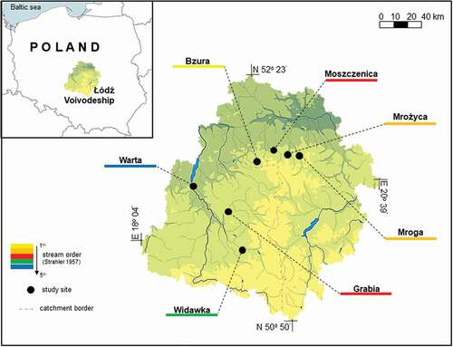
The study was performed in seven lowland rivers, i.e., the Bzura, Morga, Mrożyca, Moszczenica, Grabia, Widawka and Warta rivers, located in Central Poland (part of the Łódź Voivodeship, Poland). The region is several thousand square kilometers in area (the most distant study sites are 88 km apart), and in many respects homogenous (Figure 1). It is of geologically uniform post-glacial (Pleistocene and Holocene) origin (Przybylski et al. 2020), with several dozen to over a hundred-meter thick layer of sand, gravel or clay, and distant from mountain, marine, or large lake influences. The surroundings of the rivers are not urbanized and mostly agricultural (Grzybkowska & Głowacki 2011). However, the region is heterogeneous in certain other respects. All rivers are of different sizes (and their studied sections are of different stream orders) and differ in their hydraulic properties, substrate composition, and other environmental parameters. The first four rivers belong to the Vistula catchment, and the last three to the Oder catchment. The sampling sites, one in each river, were established in potamon river sections whose stream order (Strahler 1957) ranged from the first (the Bzura) to the fifth (the Warta) (Figure 1). Dependent on context, the name of a river is usually used as meaning “the set of assemblages sampled in the river”, or “the value of a measure/index obtained in the river”. A detailed description of all investigated study sites is presented in Table I.

Table I. Environmental parameters measured/estimated at the study sites located in seven examined rivers in Central Poland (average / coefficient of variation)

River nameCharacteristic	Bzura	Mroga	Mrożyca	Moszczenica	Grabia	Widawka	Warta
Water velocity [m s^−1]	0.24/0.18	0.06/1.69	0.06/0.17	0.04/0.61	0.36/0.35	0.37/0.31	0.40/0.23
River width [m]	0.74/0.29	3.1/0.23	4.8/0.06	3.9/0.05	15.3/0.06	27.8/0.04	57.0/0.06
River depth [m]	0.07/0.37	0.14/0.78	0.39/0.15	0.28/0.19	0.36/0.08	0.74/0.19	0.56/0.28
SI [mm]	3.4/0.66	4.9/0.46	0.4/0.33	0.3/0.04	20.8/0.22	3.9/0.13	0.8/0.15
BPOM [g m^−2]	3092/0.33	5892/0.52	7559/0.58	13951/0.21	404/0.18	1683/0.18	311/0.40
TPOM [g m^−3]	131/1.22	12/0.72	15/0.93	17/0.79	31/0.53	44/0.55	13/0.52
Water temperature [^oC]	6.7/0.75	8.9/0.49	9.8/0.53	10.9/0.65	10.8/0.61	10.2/0.73	13.7/0.53
Oxygen content [mg dm^−1]	6.1/0.36	6.8/0.31	7.2/0.27	10.5/0.20	8.6/0.28	7.9/0.30	6.9/0.28
Surface of bottom covered by SAM [%]	-	-	-	-	6.9/1.37	2.9/1.39	-

SI – inorganic substrate index, BPOM – benthic and TPOM – transported particulate organic matter, SAM – submersed aquatic macrophytes

Figure 1. Map of the study area

2.2. Field sampling

Benthic chironomid larvae with particulate organic and inorganic substrate were collected from each river once a month in an annual cycle, which produced 12 samples from each river (except the Warta, in which samples could not be collected in January and February due to ice cover; accordingly, 10 monthly samples from the Warta were obtained). The monthly sample from each river consisted of 10 sub-samples collected at sampling points established at regular distances from one another along a transect extending from the bank to the mid-channel. Each sub-sample was composed of 10 cores of benthos obtained by driving a tubular sampler 10 cm² in cross-section area 10 times into the streambed randomly around each sampling point. This was done to capture greater species diversity, and individuals were identified to the species level, if possible.

The sampler was pushed to a depth of about 150 mm, and after pulling it out each obtained core was extracted from the sampler and preserved in plastic containers with riverine water. As a result, the material of each whole monthly sample from each river consisted of 100 cores (Leszczyńska et al. 2019). Values for several environmental parameters, including water velocity [m s⁻¹], river width [m], river depth [m], surface of bottom covered by submersed aquatic macrophytes [%], water temperature [^oC] and oxygen content [mg dm⁻¹] were measured or assessed in the fields (three times per each transect).

2.3. Laboratory analysis

The samples were transported to the laboratory where they were carefully examined and invertebrates were manually sorted from benthic sediment. Chironomids were separated, preserved in 70% ethanol and identified to species level using a microscope (Nikon Eclipse 50i).

As species identification based on larval characters was not possible for some taxa, immature chironomid stages of certain species were reared in the laboratory from additional qualitative samples to obtain larval and pupal skins, and imagines. Keys written by several taxonomists and edited by Wiederholm (in three parts: for larvae (Wiederholm 1983), pupae (Wiederholm 1986) and imagines (Wiederholm 1989)), as well as a key by Nilsson (1997) were used to determine taxonomic membership. After identification, all chironomids were counted, and their density was estimated [ind. m⁻²]. Chironomids that were identified only to genus or higher taxonomic level were excluded from the statistical analysis.

The granularity of inorganic particles, using sieves of various mesh size, and inorganic substrate index, SI [mm] (Cummins 1962; Quinn & Hickey 1990), were calculated on the basis of collected samples. In addition, the amounts of benthic particulate organic matter, thereafter BPOM [g m⁻²] (Petersen et al. 1989) and transported particulate organic matter; therefore, TPOM [g m⁻³] were assessed (Grzybkowska & Witczak 1990).

2.4. Statistical methods

To produce the environmental profile of the examined rivers at the sampling sites, principal component analysis (PCA) was performed on a matrix consisting of the values of five environmental variables (water velocity, SI, BPOM, TPOM, oxygen content) × 82 monthly measurements of these variables in the seven rivers. Prior to analysis, habitat variables were tested for normality, and checked for the presence of outliers. Diagnostic plots of residuals against fitted values and normal QQ plots of residuals were used to assess assumptions of normality. The environmental profile was obtained by a reduction of the five entry variables to a limited set of uncorrelated components (PC axes). However, only PC axes with eigenvalues >1 (the Kaiser criterion) were used in further analysis. The interpretation of each selected component (PC axis) was made on the basis of correlations (loads) between the component and original variables. One-way analysis of variance (ANOVA I) and Fisher’s Least Significant Difference (LSD) post-hoc test were performed, separately for each PC component, to find differences among rivers in the environmental profile. To detect the resemblance between particular rivers cluster analysis with Pearson correlation as a criterion of similarity and UPGM as a method of clustering were used. The measure was applied to the density matrix of averaged chironomid species’ densities in given rivers. All statistical analyses were performed in Statistica 13 software (Dell Inc 2016). Probability values P < 0.05 were considered significant. Data are reported as mean ± standard error (SE).

One-way permutational analysis of similarity, i.e., ANOSIM, a test of significant difference between groups of sites/samples, was adopted as a method of assessing river similarities. Bray-Curtis was the applied measure of similarity between assemblages (Clarke 1993; Clarke & Warwick 2001). ANOSIM is analogous to an ANOVA procedure, with a non-parametric permutation (10,000 permutations were used) applied to a rank similarity matrix of samples (Clarke 1993). In this procedure, the R statistic provides an absolute measure of how groups are separated. Generally, R values lie between 0, when groups are indistinguishable, and +1, when all similarities within groups are less than the similarity between groups (Clarke & Warwick 1994). When the overall difference was significant, indicating which riverine sets of assemblages were different from others, the pairwise ANOSIM comparisons were performed and P-values were determined based on a step-down sequential Bonferroni procedure.

SIMPER, a percentage similarity analysis, was used to identify which taxa were primarily responsible for the observed differences between assemblages (Clarke 1993). Similarly to ANOSIM, the Bray-Curtis assemblage similarity measure was used for SIMPER analysis. Only species whose cumulative contribution to overall dissimilarity was equal to or higher than 60% were considered. ANOSIM and SIMPER analyses were conducted using the PAST v3.26 software (Hammer et al. 2001; Hammer 2019).

A number of univariate alpha diversity indices were applied to assess the within river characteristics. To avoid spurious conclusions that may result from a narrow choice of such indices (Magurran & McGill 2011) the present selection was comprehensive, because it included species richness, entropy used as a diversity index, dominance index, and two evenness indices. The indices were:

Hill numbers N₀, N₁, N₂, i.e.

$N_0=\sum {p_i}^0=S$

$N_1=exp\left(-\sum p_i\mathrm{l}\mathrm{n}{p}_i\right)=e^{H^{\mathrm{\prime }}}$

$N_2=1/\sum {p_i}^2$ (Hill 1973)

Shannon $H\prime =-\sum p_i\text{ln}{p}_i$ (Shannon & Weaver 1949)

Pielou J’ $=$ H’/lnS (Pielou 1966)

$\mathrm{S}\mathrm{i}\mathrm{m}\mathrm{p}\mathrm{s}\mathrm{o}\mathrm{n}\lambda ={{\sum p}_i}^2$(Simpson 1949)

BGS$=$ e${ }^{H^{\mathrm{\prime }}}$/S (Buzas & Gibson 1969; Sheldon 1969)

where: p_i – the proportion of individuals belonging to the ith species in the dataset, S – species richness.

The univariate alpha diversity indices were calculated for each monthly sample obtained in each river over the annual cycle. As a result, in the case of each diversity index, we obtained a set of 10 values for the Warta River, and sets of 12 values for each other river. Because the distributions of the values of each index were unknown we could not average the values for each river to compare them. Instead, we bootstrapped each set of monthly values. One hundred pseudo-samples were produced for each index and each river to obtain normal distributions of data sets. This number of pseudo-samples was selected to avoid spurious small or large sample effects on the significance of the comparison of the means of bootstrap pseudo-samples using the ANOVA test: i.e., Type I and Type II errors (Fritz et al. 2012; Khalilzadeh & Tasci 2017). The bootstrap sets for each index were then compared using ANOVA. A post-hoc Tukey test was used to distinguish homogenous groups of assemblages/rivers of each index.

However, beside the above stand-alone alpha diversity assessment of given rivers, diversity was also calculated as a multiplicative partitioning/decomposition paradigm. In this paradigm, the average alpha and beta components are calculated for neither a specific assemblage nor river, but for the whole region. When multiplied by each other these average alpha and beta components create gamma, total regional diversity (Whittaker 1960). In the case of N₀ and N₁, the respective formulas are (modified from Jost 2007):

$\begin{array}{rl}& N_0\mathrm{a}\mathrm{l}\mathrm{p}\mathrm{h}\mathrm{a}=\left(\frac{1}{\mathrm{M}}\right)\left[\left(\sum _{i=1}^s{S}_{i1}\right)+\left(\sum _{i=1}^s{S}_{i2}\right)+\cdot \cdot \cdot +\left(\sum _{i=1}^s{S}_{i\mathrm{M}}\right)\right]\\ & N_0\mathrm{g}\mathrm{a}\mathrm{m}\mathrm{m}\mathrm{a}=\sum _{i=1}^s{S}_i\\ & N_0\mathrm{b}\mathrm{e}\mathrm{t}\mathrm{a}=N_0\mathrm{g}\mathrm{a}\mathrm{m}\mathrm{m}\mathrm{a}/N_0\mathrm{a}\mathrm{l}\mathrm{p}\mathrm{h}\mathrm{a}\\ & N_1\mathrm{a}\mathrm{l}\mathrm{p}\mathrm{h}\mathrm{a}=exp\left[-w_1\sum _{i=1}^s\left(p_{i1}ln{p}_{i1}\right)+-w_2\sum _{i=1}^s\left(p_{i2}ln{p}_{i2}\right)+\cdot \cdot \cdot \right]\\ & N_1\mathrm{g}\mathrm{a}\mathrm{m}\mathrm{m}\mathrm{a}=exp\left[\sum _{i=1}^s-\left(w_1{p}_{i1}+w_2{p}_{i2}+\cdot \cdot \cdot \right)\times ln\left(w_1{p}_{i1}+w_2{p}_{i2}+\cdot \cdot \cdot \right)\right]\\ & N_1\mathrm{b}\mathrm{e}\mathrm{t}\mathrm{a}=N_1\mathrm{g}\mathrm{a}\mathrm{m}\mathrm{m}\mathrm{a}/N_1\mathrm{a}\mathrm{l}\mathrm{p}\mathrm{h}\mathrm{a}\end{array}$

where S is the number of species of a given assemblage, p_i is a proportion of the density of species i in a given assemblage, w is the weight of a given assemblage in the set of compared assemblages, and M is the number of assemblages (all logarithms are to the base e). Note than N₀ gamma diversity is calculated from the pooled assemblages; hence in the gamma calculation S refers to the number of species in that pool. The alpha and gamma are in number of species, while the beta in number of assemblages. The possible range of the beta component is between unity, when all assemblages are identical, and the total number of assemblages, when each and every assemblage contains all different species. In this study, we calculated the average alpha and beta components for all 82 assemblages. This was done in the case of only these indices, in which meaningful decomposition might be carried out, i.e., N₀ and N_1. The partitioning of the N₁ index was applied in Głowacki & Penczak (2013).

3. Results

In total, 61 chironomid species from 5 subfamilies (Tanypodinae, Diamesinae, Prodiamesinae, Orthocladiinae, Chironominae) were identified in the studied streams. An additional 8 genera were also recorded (Procladius, Paraphaenocladius, Orthocladius, Parametriocnemus, Corynoneura, Psectrocladius, Saetheria, Rheotanytarsus) though it was impossible to identify these taxa to the species level. The highest total numbers of species, above 30, were found in the Grabia, Widawka and Moszczenica Rivers, while the lowest, with 14 species, was in the Bzura River (Table II).

Table II. The list of identified chironomid species with their mean density (ind. m⁻²), standard deviations (sd), occurrence frequencies (f) and total number of species from seven examined rivers in Central Poland

	Bzura			Mroga			Mrożyca			Moszczenica			Grabia			Widawka			Warta
	mean	sd	f	mean	sd	f	mean	sd	f	mean	sd	f	mean	sd	f	mean	sd	f	mean	sd	f
Tanypodinae
Ablabesmyia monilis (Linnaeus, 1758)										56	153	0.3	49	48	0.8	41	42	0.8	14	29	0.4
Anatopynia plumipes (Fries, 1823)										2	8	0.1
Apsectrotanypus trifascipennis (Zetterstedt, 1838)							2	5	0.1				1	2	0.1
Conchapelopia melanops (Meigen, 1818)	309	518	0.7	30	43	0.4	2	5	0.1	1	3	0.1	2	6	0.1	2	5	0.2
Macropelopia nebulosa (Meigen, 1804)	6	21	0.1	44	55	0.6	31	41	0.6	180	188	0.8	1	3	0.1
Natarsia punctata (Fabricius, 1805)*													1	3	0.1	2	7	0.2
Diamesinae
Potthastia gaedii (Meigen, 1838)				16	43	0.3							6	9	0.4	2	6	0.1
Potthastia longimanus Kieffer, 1922												0.0	38	61	0.7	33	49	0.6	3	5	0.3
Prodiamesinae
Monodiamesa bathyphila (Kieffer, 1918)				19	25	0.4	38	52	0.7				18	29	0.7	8	10	0.6
Odontomesa fulva (Kieffer, 1919)				158	318	0.6	23	29	0.5	2	6	0.2	20	27	0.6	19	29	0.6
Prodiamesa olivacea (Meigen, 1818)	2762	2871	0.9	830	766	0.9	714	571	0.8	125	225	0.8	14	12	0.7	254	265	1.0	2	3	0.4
Prodiamesa rufovittata Goetghebuer, 1932													15	27	0.6	9	9	0.7
Orthocladiinae
Brillia bifida (Kieffer, 1909)*							6	16	0.2
Brillia flavifrons (Johannsen, 1905)*							5	16	0.1	1	3	0.1
Brillia longifurca Kieffer, 1921*													31	83	0.3	9	15	0.3
Cricotopus bicinctus (Meigen, 1818)*										1	3	0.1	13	20	0.4	13	20	0.4	125	398	0.8
Cricotopus sylvestris (Fabricius, 1794)*										3	6	0.2	1840	1973	1.0	193	186	1.0
Diplocladius cultriger Kieffer, 1908													9	28	0.2
Epoicocladius ephemerae (Kieffer, 1924)							2	5	0.1
Eukiefferiella brevicalcar (Kieffer, 1911)*												0.0	36	43	0.6	30	25	0.9
Eukiefferiella gracei (Edwards, 1929)*													1079	997	1.0	4	5	0.5	1	2	0.1
Eukiefferiella sp. 1	3	11	0.1
Eukiefferiella sp. 2																2	6	0.1
Heterotrissocladius marcidus (Walker, 1856)*	3	11	0.1				72	109	0.5			0.0	55	69	0.7	2	6	0.2
Heterotrissocladius subpilosus (Kieffer, 1911)*				11	33	0.2	17	58	0.1
Nanocladius rectinervis (Kieffer, 1911)				4	11	0.2							22	48	0.3				3	9	0.2
Parakiefferiella bathophila (Kieffer, 1912)																2	6	0.2
Paratrichocladius rufiventris (Meigen, 1830)																2	5	0.2
Rheocricotopus fuscipes (Kieffer, 1909)	3	11	0.1										20	31	0.4
Synorthocladius semivirens (Kieffer, 1909)*							2	5	0.1				55	76	0.5	16	31	0.5
Thienemanniella clavicornis (Kieffer, 1911)*													1	4	0.1	16	23	0.5
Thienemannia gracilis Kieffer, 1909										3	8	0.2							3	8	0.2
Tvetenia calvescens (Edwards, 1929)*										1	3	0.1	20	32	0.4
Chironominae/Chironomini
Chironomus riparius Meigen, 1804	7645	6992	1.0	11	23	0.3	2	5	0.1	310	742	0.8				625	671	0.9	2	6	0.1
Chironomus sp. 1										30	53	0.3
Cryptochironomus borysthenicus (Chernovskij, 1949)							17	58	0.1	50	84	0.4	10	23	0.2				57	92	0.4
Cryptochironomus defectus (Kieffer, 1913)	3	11	0.1				29	47	0.6	38	42	0.8	292	312	1.0	103	112	0.9	1	3	0.2
Cryptochironomus supplicans (Meigen, 1830)*										21	28	0.5
Dicrotendipes nervosus (Staeger, 1839)	6	14	0.2							1	3	0.1							33	88	0.4
Endochironomus albipennis (Meigen, 1830)										12	38	0.2							1	2	0.1
Endochironomus sp. 1				3	11	0.1
Endochironomus sp. 2				15	33	0.3
Endochironomus sp. 3																			2	8	0.1
Glyptotendipes cauliginellus (Kieffer, 1913)	3	11	0.1							7	13	0.3							25	38	0.8
Glyptotendipes paripes (Edwards, 1929)				3	11	0.1
Microtendipes chloris (Meigen, 1818)				48	62	0.5	232	386	0.8	60	118	0.6							36	50	0.6
Parachironomus gracilior (Kieffer, 1918)							2	5	0.1	1	4	0.1				1	4	0.1	3	9	0.1
Paracladopelma camptolabis (Kieffer, 1913)*				7	21	0.2	26	42	0.4				11	25	0.2	62	59	0.9	12	40	0.2
Paratendipes albimanus (Meigen, 1818)*	6	14	0.2	62	158	0.3	179	383	0.4	744	1257	0.6	46	94	0.3	2	5	0.2	82	170	0.5
Paratendipes connectens Lipina, 1926*										7	23	0.1							196	432	0.6
Polypedilum convictum (Walker, 1856)*							2064	1656	1.0	19	43	0.3	1071	1186	1.0	1017	485	1.0	1	4	0.1
Polypedilum nubeculosum (Meigen, 1804)*	6	14	0.2							120	213	0.6	38	39	0.8	34	39	0.8	2	4	0.2
Polypedilum pedestre (Meigen, 1830)*							2	5	0.1	1	4	0.1				17	16	0.8	4	13	0.1
Polypedilum scalaenum (Schrank, 1803)*	3	11	0.1	38	50	0.5	1589	1419	1.0	1102	2379	0.9							1	3	0.2
Robackia demeijerei (Kruseman, 1933)										11	33	0.2							764	642	1.0
Stictochironomus sticticus (Fabricius, 1781)	3	11	0.1	275	229	0.9	434	390	0.8			0.0	138	192	0.7	65	80	0.8	3	9	0.2
Chironominae/Tanytarsini
Cladotanytarsus mancus (Walker, 1856)*				12	42	0.1	162	522	0.2	11	20	0.3	2436	1620	1.0	254	192	1.0
Micropsectra notescens (Walker, 1856)*	2166	641	0.2	79	74	0.8	3697	6313	0.9	3	5	0.3	323	313	0.9	41	37	0.9
Paratanytarsus dissimilis (Johannsen, 1905)*													3	5	0.3	102	94	1.0	339	816	1.0
Paratanytarsus sp. 1				15	53	0.1				18	62	0.1
Tanytarsus gregarius Kieffer, 1909*													384	386	0.8	2	5	0.2	1	4	0.1

* reared in the laboratory

The most frequent species in chironomid assemblages were: Prodiamesa olivacea, Polypedilum convictum, Polypedilum scalaenum, Micropsectra notescens, Chironomus riparius and Robackia demeijerei. Subdominants, which were present in more than one stream, but in different densities, were Paratendipes albimanus (Mrożyca, Moszczenica, Warta), Stictochironomus sticticus (Mroga, Mrożyca), and Cladotanytarsus mancus (Grabia, Widawka).

The environmental profile of the rivers is presented in Figure 2. Each point of the figure represents a multidimensional environmental condition in which a respective chironomid sample was collected. The PCA allowed a reduction of the five environmental variables to two orthogonal axes (PC 1 and PC 2) with eigenvalues higher than unity. These two axes explained 64.75% of the total variance (Figure 2). The correlation between the abundance of particular environmental variables and the new components revealed that the first axis (PC 1) represents a gradient extending from decreasing water velocity and SI to increasing amount of BPOM. The second axis (PC 2) represents a gradient extending from declining oxygen concentration to growing amount of TPOM.

Figure 2. Habitat profile of examined rivers in Central Poland depicted by PC scores (average ± standard error). Values of loadings (Pearson correlations) of environmental parameters are in bold, % of the total variance explained by PC axes are in brackets. VEL – velocity; SI – inorganic substrate index; BPOM, TPOM – benthic, transported particulate organic matter; OXY – oxygen

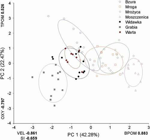
Analysis of variance showed that the examined rivers differ significantly (F_6,73 = 95.58, P < 0.001) in PC 1 scores, and the multiple comparison LSD post-hoc test identified five homogenous groups, i.e., Grabia, Warta = Widawka = Bzura, Mroga, Mrożyca, Moszczenica. Similar differences in the environmental profile were also noted for PC 2 scores (F_6,73 = 12.76, P < 0.001), where four homogenous groups: Grabia, Moszczenica = Widawka, Widawka = Mroga = Mrożyca = Warta, Bzura, were distinguished. The Widawka River cannot be precisely situated (and thus should be considered belonging to no group), because it belongs to two homogenous groups simultaneously (Zar 2010).

Based on species abundance in the examined rivers, three main clusters were identified (Figure 3). Streams of lower orders (the Bzura, Mroga, Mrożyca and Moszczenica) formed the first cluster (separated at a distance of 0.53). The second cluster comprised two larger rivers: the Grabia and Widawka (separated at a distance of 0.67). The chironomid assemblage of the Warta River, the largest river in Central Poland, was the most different from the other assemblages (at a distance of 0.79), constituting a separated branch (and the third cluster) in the dendrogram.

Figure 3. Clusters of chironomid abundance in the examined rivers of Central Poland obtained using the UPGM method and Pearson correlation as a similarity index

The chironomid assemblages differed significantly using the ANOSIM measure (R-statistic = 0.8817, P<0.001), and pairwise comparisons revealed that each river differed significantly from all the others (Table III). Moreover, SIMPER analysis indicated that overall dissimilarity among the rivers was 76.9%, and 14 of the total of 61 species produced over 57.3% of cumulative dissimilarity (Table IV). Seven of the 14 species (C. riparius and P. olivacea in the River Bzura, P. scalaenum and P. convictum in the Mrożyca, M. notescens in the Moszczenica, and P. albimanus, and C. mancus in the Grabia) were the most abundant ones (usually over 4500 ind. m⁻² in each waterbody). Moreover, these species were the most frequent chironomids in the whole dataset. The seven species produced over 33.7% of cumulative dissimilarity and could be related to significant differences in the chironomid assemblages (Table IV).

Table III. Bray-Curtis overall dissimilarity between the structures of given chironomid assemblages that was received from ANOSIM analysis (above the diagonal) and probability of Bonferroni pairwise post-hoc comparisons (below the diagonal)

River	Bzura	Mroga	Mrożyca	Moszczenica	Grabia	Widawka	Warta
Bzura		72.76	82.44	74.81	92.29	76.44	94.54
Mroga	0.0001		57.72	74.64	82.00	76.53	91.84
Mrożyca	0.0001	0.0001		67.76	68.39	85.45	89.09
Moszczenica	0.0001	0.0001	0.0001		82.14	75.47	83.47
Grabia	0.0001	0.0001	0.0001	0.0001		47.64	89.35
Widawka	0.0001	0.0001	0.0001	0.0001	0.0001		82.66
Warta	0.0001	0.0001	0.0001	0.0001	0.0001	0.0001

Table IV. Given species’ contribution to overall dissimilarity among the chironomid assemblages of the seven examined rivers in Central Poland obtained from SIMPER analysis

Taxon	Average dissimilarity	Contribution %	Cumulative contribution %
C. riparius	4.717	6.131	6.131
P. convictum	4.201	5.460	11.59
P. olivacea	3.963	5.150	16.74
P. scalaenum	3.656	4.751	21.49
M. notescens	3.651	4.745	26.24
S. sticticus	3.399	4.418	30.65
C. mancus	3.118	4.053	34.71
C. defectus	2.711	3.523	38.23
P. albimanus	2.643	3.436	41.67
C. sylvestris	2.614	3.397	45.06
M. chloris	2.511	3.263	48.33
M. nebulosa	2.388	3.104	51.43
P. dissimilis	2.312	3.005	54.44
R. demeijerei	2.211	2.873	57.31

Univariate alpha species diversity indices (species richness, diversity per se, Shannon entropy, Simpson domination and evenness indices) (Figure 4) showed that variation occurred both from index to index and from river to river. Besides, there were only five two-river homogeneous groups in all the seven indices, one three-river group, and two two-river groups that overlapped. In two indices, all rivers were completely heterogeneous (i.e., each river constituted a different group).

Figure 4. Means (and their standard deviation - whiskers) of bootstrap pseudo-samples of species richness, diversity per se, dominance and evenness indices calculated for sets of chironomid assemblages in each studied river. Simple ANOVA was used to assess if the means of the rivers differed significantly. Letters at the standard deviation values indicate homogeneous groups in each index. The units of the y axes of N₀, N₁, and N₂ indices are numbers of species. The units of the y axes of the remaining indices are abstract numbers

In N₀ of the multiplicative partitioning/decomposition paradigm, the gamma diversity of the region amounted to 61 species, the average alpha component to 11.00 species, and the beta component to 5.50 assemblages. In N₁ of the paradigm, the gamma diversity of the region amounted to 18.31 species, the average alpha component to 4.04 species, and the beta component to 4.53 assemblages.

4. Discussion

4.1. General chironomid abundance and assemblage structure in comparison to other parts of the world

The composition of chironomid assemblages inhabiting all the study rivers was typical for lowland waterbodies from the Palaearctic zone (Pinder 1995; Ferrington 2008). In such rivers, the chironomid fauna of a rhithral section (Armitage et al. 1995; Andersen et al. 2013) is usually dominated by the subfamily Orthocladiinae and other taxa preferring cool, well-oxygenated environments. Meanwhile, the dominant chironomid fauna in potamal river sections are representatives of the Chironomini (subfamily Chironominae). Generally, species of the latter subfamily live in soft sediment and present a wide range of tolerance, especially in terms of higher water temperature and lower oxygen concentrations (Armitage et al. 1995). Stream order also seems to be of importance here. Lower order sections are usually populated by many Prodiamesinae and a few Chironomini species, while higher-order sections by many Chironomini, Tanytarsini and Orthocladiinae (Vannote et al. 1980). This was also the case in the present investigations.

The highest abundance or species richness of the genera Chironomus and Polypedilum, which were also the most abundant in our investigation, was observed in chironomid assemblages from lowland rivers both in Europe (Árva et al. 2017) and in other continents (Ashe et al. 1987; Armitage et al. 1995; Chaib et al. 2013). In the study of the Arkansas River basin (USA) conducted by Herrmann et al. (2016), for example, 12 species of Polypedilum and 11 species of Chironomus were recorded. Moreover, Chironomus decorus was the most common species that appeared at all their study sites, excluding one. In turn, in the floodplain of the Paraná River (Brazil), larvae of Polypedilum were the subdominant component of chironomid assemblages (Tanytarsus dominated). Two species of Chironomus were also mentioned as those with high density (Júnior et al. 2016). In the Phong River in Thailand, Polypedilum nubifer constituted more than one-fourth of the assemblage (Sriariyanuwath et al. 2015). In the African Swartkops River, Odume et al. (2011) also indicated Chironomus and Polypedilum (tribe Chironomini) as two of the five most abundant taxa.

In general, in the temperate regions, the species richness of Chironominae and Orthocladiinae subfamilies amounts to 30% each of the total number of species (Thienemann 1954; Cummins & Lauff 1969; Tolkamp 1982; Armitage et al. 1995; Pinder 1995; Bournaud et al. 1998; Andersen et al. 2013). In our study, the percentage of Chironomini species was even higher and constituted about 47% of the total number of species, while that of Orthocladiinae about 33%. However, in the case of density, Orthocladiinae larvae were not numerous and can be treated here as rare species, in contrast to ecosystems rich in submersed aquatic macrophytes where they are present at high densities, mostly because many of them are grazers or scrapers (Grzybkowska et al. 2017, 2020).

The remaining chironomid subfamilies, Tanypodinae, Prodiamesinae and Diamesinae, assumed the values of 10%, 7%, 3%, respectively. The density of Tanypodinae usually displays high fluctuations between study sites, and this is typical for most non-disturbed rivers (Rossaro 1991). Prodiamesinae were represented mainly by P. olivacea, which rarely is the dominant component of chironomid assemblages, except the Bzura River in Central Poland (Grzybkowska 1995). In the Zwalm River in Belgium, for instance, it was the most common species present at all examined sites (Adriaenssens et al. 2004), whereas the sub-family Diamesinae was represented by only two species, Potthastia longimanus and Potthastia gaedii, which are two of the most flexible taxa of this subfamily (in both rhithral and potamal sections of streams and rivers; Moubayed-Breil & Orsini 2016). In general, this occurrence of the two Potthastia species is in contrast to other geographical areas or altitudes, because Diamesinae, and especially the genus Diamesa, are the first taxa that colonize streams immediately downstream of source glaciers (Lencioni & Rossaro 2005). They are cold-stenobionts that prefer low water temperature and fast flowing streams, where they are usually the dominant component of assemblages (Rossaro 1991; Lods‐Crozet et al. 2001).

4.2. Distance between chironomid assemblages in view of the riverine environmental profile of the region

The habitat heterogeneity of streams is considered as one of factors that are of key importance in determining the occurrence and distribution of aquatic invertebrates (Thienemann 1954; Hynes 1970; Coffman 1989; Malmqvist 2002; Costa & Melo 2008; Júnior et al. 2016). However, dependent on the scale of a study, geographical localisation of investigated areas, etc., different environmental parameters are distinguished as those that explain the majority of total variation between chironomid assemblages. Numerous studies conducted worldwide at the regional or local scale in the latest two decades indicate the following factors as most important: water temperature (Lencioni & Rossaro 2005; Marziali & Rossaro 2013), discharge or current velocity (Fesl 2002; Karaouzas & Płóciennik 2016), inorganic bottom substrate (Grzybkowska & Witczak 1990; Chaib et al. 2013; Leszczyńska et al. 2019), organic matter (König & Santos 2013; Mauad et al. 2017), dissolved oxygen (Özkan et al. 2010; Leszczyńska et al. 2017), physicochemical parameters (Chaib et al. 2013) and channel morphometry (Karaouzas & Płóciennik 2016).

To some extent, the lack of agreement as regards which environmental factor is the most important may result from a hierarchical impact of some factors, and a tendency of some authors to believe that a specific level is more significant than others. Inorganic bottom substrate, for example, can be essential for supplying macroinvertebrates with place to inhabit and refuge against predators. Yet, inorganic bottom composition is affected by water velocity, similarly as the transfer of organic particles (in the form of detritus, for example, which represents the basic food resource of many taxa (Graça et al. 2004)), the mobility of drifting organisms, and the level of dissolved oxygen, which in turn controls basic life processes (Matthaei et al. 1997).

The environmental profile of our region (Figure 2) was created to determine to what extent the environmental conditions differed among our rivers. Each of the ellipses of the figure is a 95% prediction area where the points of multidimensional environmental variables’ values of each river would occur. The general arrangement of the ellipses is ecologically informative because each of them either overlap or adjoin, and thus they all form a single connected group. Consequently, the regional environmental conditions of the sampled chironomid assemblages were relatively homogeneous. If any of the ellipses had been disconnected from others, this would have indicated that the conditions of the region were more heterogeneous.

Environmental conditions that were average for the region occurred at the crossing of the zero points of both PC axes; hence, the farther an ellipsis was located from the crossing the more the conditions of its river differed from the average regional values. The ellipses also considerably differed in size of area and in elongation. The conditions of small ellipses represented rivers whose environmental variables’ values little varied over the year in which the river’s chironomid assemblages were sampled. Large but non-elongated ellipses represented rivers whose all environmental variables’ values considerably varied over the sampling year, but according to no obvious pattern. In contrast, the strongly elongated ellipsis of the Bzura River indicated that the river’s conditions varied strongly, but in a specific way: when the values of some variables kept on decreasing, the values of other variables kept on increasing.

The two measures used to assess distances between the rivers in terms of their chironomid assemblages (ANOSIM and clustering) indicated several phenomena. ANOSIM showed that distances within each pair of the rivers were highly significant, but the distances also differed considerably from pair to pair (between 47.64% and 94.54%, values close to 100% indicating greatest difference between given rivers’ chironomid assemblages). Similar ANOSIM values at the regional scale were also obtained by other chironomid researchers (Odume et al. 2011; Robinson et al. 2016). The method of clustering confirmed the varying distances, because the rivers of the tightest pair were at the distance of 0.27, while the most distant rivers at 0.79 (range 0–1). There was a considerable congruence between the patterns of environmental distances as expressed by the environmental profile of the region and the chironomid patterns between the rivers as presented by the ANOSIM and clustering methods.

Because SIMPER analysis indicated that 14 of the total of 61 species produced over 57.3% of cumulative dissimilarity (Table IV), the rest of the species (47) accounted for 43% of variability. And thus each of the latter explained on average less than 0.91%. Meanwhile each of the 14-species group explained on average as much as 4.07%, the differences within the 14-species group being moderate (range: 2.873–6.131). As many as 11 species of the 14-species group are of the subfamily Chironominae (eight of the Chironomini tribe, and three of the Tanytarsini tribe). This indicates that this subfamily responds much stronger to the environmental profile of our region than other tribes and subfamilies. However, it is noticeable that the decline in the percentage of differences between assemblages explained by given species is less steep than occasionally recorded elsewhere. Among 40 chironomid species in Alpine streams, for example, two species of Orthocladius sp. (juv.) and Diamesa zenyi-cinerella gr. explained 28.8%, while six species 59.5% of total variability (Robinson et al. 2016). Among 26 species recorded in four sites of the lowland Swartkops River (South Africa), the species of Chironomus sp. 1 and Dictotendipes sp. explained 52.3% of total variability (Odume et al. 2011).

Seven of the 14 species, C. riparius, P. convictum, P. olivacea, P. scalaenum, M. notescens, S. sticticus and C. mancus, were most important and most abundant in our investigations. This is why some of them and also some of the other seven are characterised here in more detail. C. riparius and P. olivacea were the most abundant in low order streams, with low velocity and dense riparian vegetation. Both these chironomid species prefer stagnant water and soft sediments. Soft sediments are necessary for C. riparius not only as a food resource, because it has the ability to feed both as a gathering-collector and as filtrator, depending on the availability of food particles (Walshe 1951), but also to build tubes, in which it lives (Wiederholm 1983). It is also well known owing to its efficient oxygen regulation, thanks to which it may inhabit organically enriched and heavily polluted waterbodies (Connolly et al. 2004; De Haas et al. 2004). Moreover, we noticed in our many previous studies, that when C. riparius was absent in muddy substrate, larvae of M. chloris often appeared instead. Probably larvae of M. chloris are more stenobiontic and have less competitive power. In turn, P. olivacea demands a portion of the leaf packages in addition to soft sediment, on the surface of which it feeds (Lindegaard-Petersen 1972; Moller Pillot & Buskens 1990; De Bisthoven et al. 1992).

P. convictum and P. scalaenum together with M. notescens are considered as eurytopic and tolerant species (Wiederholm 1983; Boesel 1985; Herrmann et al. 2016). Both species of Polypedilum produce silken tubes in silt, sand or in plant tissues, feeding mostly on plankton. Larvae of these taxa are also known to occupy cases of caddisflies (Boesel 1985). Alternate high and low density of these two taxa in the examined rivers can indicate the possibility of some interaction between the two ecologically relatively close species. M. notescens also builds tubes but it is able to occur even in extreme environments (Wiederholm 1983). The presence of these three species can be connected to very high quantity of organic matter, useful to construct their tubes, or to unidentified and uncontrolled inflow of pollution, which allows only resistant species to survive in the environment.

Fine bottom substrate and quite fast water velocity, which creates an unstable substrate, is avoided by many species, but notable exceptions are to be found in the orthoclad genus Rheosmittia and among the so-called Harnischia group of genera (Armitage et al. 1995). In our study, such sandy habitat was inhabited by one of the species from the Harnischia group – R. demeijerei. In the Warta River, it dominated in homogenous sandy bottom in the mid-channel. S. sticticus is believed to inhabit rivers with sandy habitats and a low current speed (Wiederholm 1983). Yet, in our study, it was present in different habitats with low and fast velocity and fine and coarse granulometrity of inorganic bottom. C. mancus is considered as a typical, eurytopic filtrator that builds tubes (Wiederholm 1983). However, in our study, its sensitivity to decreased level of oxygen and transported particulate organic matter was observed. C. sylvestris is one of those Orthocladinae species that well cope with high amplitude of discharge, well-oxygenated water, coarse substrate and presence of macrophytes (Wiederholm 1983).

4.3. Univariate alpha species diversity (species richness, diversity per se, entropy as diversity, dominance, and evenness) measures of the studied rivers

The univariate diversity indices that we apply here are non-parametric, i.e., not related to the species abundance distribution (SAD) underlying the assemblage that a measure describes (similarly as the clustering and ANOSIM measures). Yet, in contrast to the clustering and ANOSIM measures, which present the compositional distance of each and every river from all the other rivers in an abstract space, and are thus relative, the diversity indices are absolute, and thus constitute stand-alone assessments (McGill et al. 2007).

However, the univariate diversity indices display only that part of diversity (or concentration or evenness) that occurs within given rivers, i.e., the alpha component. This part may be averaged and joined to the beta component (between rivers) to create gamma diversity (Whittaker 1960), i.e., diversity of the region. This estimate is provided in the case of N₀ and N₁ (see Results), though the average alpha, beta and gamma diversity is calculated for the 82 assemblages instead of the seven rivers.

In Figure 4, rivers are arranged in each index according to increasing stream orders and the values of the rivers vary both within and between indices. In the case of species richness, diversity per se and Shannon entropy, the rivers present a humpback pattern, with the first and last rivers being the lowest values (or almost the lowest, as in N₀). In the Simpson concentration, the pattern is a vertical mirror image of the humpback pattern, with the first and last rivers being the highest values. Lack of a clear pattern occurs in the two evenness indices, although for the Pielou evenness the first and last rivers are also the lowest values.

In N₀, the values accord with previous studies (Coffman 1989), where an increase in species richness is recorded from stream order 1 through order 3, and stabilization occurs in higher orders. In contrast, in the Warta a clear decrease occurred. This finding is, however, in accordance with the results of other studies conducted worldwide, which indicate that an abrupt change in macroinvertebrate assemblages may frequently be noted in the 4th- and/or 5th-order streams (Hynes 1970; Minshall & Robinson 1998; Clarke et al. 2008; Melo 2009).

The pattern of N₀ was modified in the diversity per se and Shannon indices in such a way that the hump became gradually level, although not to an extent that would make the pattern unidentifiable. This levelling off was an effect of numerous factors, with the most important the decreasing impact of rare species, for instance, from genera Epoicocladius and Eukiefierella and increasing impact of abundant species from index to index.

The values of the two evenness indices (BGS and Pielou) were unexpected, being greatly different from those in the remaining five indices and from each other. While the BGS index distinguished a homogenous group of three rivers (the Grabia, Widawka, and Warta), each of the rivers belonged to a different group in the Pielou index. This result of the BGS index may be explained if we remember that the index is also the ratio of N₁/N₀ (or N₁/S). The respective divisions are as follows:

Grabia: 5.768(N₁)/17.716(N₀) = 0.3256

Widawka: 6.725(N₁)/18.846(N₀) = 0.3568

Warta: 3.166(N₁)/9.339(N₀) = 0.3390.

The results are so similar that the ANOVA (applied to bootstrap pseudo-samples) post-hoc test ascribed the three rivers to one group. The results are understandable because the ratios of these three rivers in N₁ and N₀ are similar. Conversely, in the Pielou index, which is the ratio of the Shannon index to the natural logarithm of N₀, it was not the case. Although the Shannon index ratio of these three rivers is also similar to that in N₁, yet the lnN₀ values of the rivers are now greatly changed; hence, the outcomes of divisions are also different from those in the BGS index. Inspect related calculations:

Grabia: 1.724(Shannon)/2.8744(lnN₀) = 0.5998

Widawka: 1.853(Shannon)/2.936(lnN₀) = 0.6311

Warta: 1.112(Shannon)/2.234(lnN₀) = 0.4977

which explain why the ANOVA post-hoc test ascribed all three rivers to different groups each. Note that a disparity as small as 1.13 species (between the Grabia and Widawka) was enough to effect a significant difference.

But reverse outcomes as regards the impact of difference in species number also occurred. In the Pielou index, differences as large as 5.482 species (the Bzura and Warta) and even 7.557 species (the Mrożyca and Grabia) were not large enough to ascribe rivers of each of these pairs to different groups. Consider the related calculations, in which the results of divisions in the former pair and in the latter pair are similar:

Bzura: 0.636(Shannon)/1.3499(lnN₀) = 0.4711

Warta: 1.112(Shannon)/2.2342(lnN₀) = 0.4977

Mrożyca: 1.423(Shannon)/2.3184(lnN₀) = 0.6138

Grabia: 1.724(Shannon)/2.8744(lnN₀) = 0.5998.

In other words, if we had relied on the BGS index only, we would have concluded that the Grabia, Widawka and Warta were quite similar to one another, while all the other rivers greatly different. Conversely, if we had relied on the Pielou index only, we would have concluded that only the Warta and Bzura, and also the Mrożyca and Grabia were similar to each other, while the Grabia, Widawka and Warta were not. Note that both the Pielou and BGS indices are perfect evenness indices (Jost 2010). However, they indicate different aspects of evenness.

These different aspects have been identified only recently. For many previous decades, the BGS index was considered superior to the Pielou, because the former is replication invariant, i.e., does not change its value when the index is applied to a dataset that consists of the original assemblage pooled with its copy (as regards SAD) that includes all different species (Taillie 1979; Alatalo 1981), while the Pielou index does change. Jost’s (2010) analysis indicated that a change of perspective renders the importance of the two evenness indices differently. BGS gives the absolute evenness and inequality: when the number of species is higher, a maximally unequal assemblage shows more absolute inequality (less absolute evenness) than when the number of species is low. In contrast, the values of the Pielou index remain correct relative to the possible range of evenness at a given number of species. Consequently, the Pielou index should be considered the ideal relative evenness index (Jost 2010).

To conclude, on the basis of complex analysis of both relative and absolute measures, we observed that investigated chironomid assemblages’ composition in rivers located in a quite homogenous area of Central Europe reflected the environmental profile of the region. This homogeneity seems to be related to rather common and eurytopic than rare species, i.e., P. olivacea (Prodiamesinae), C. riparius, P. scalaenum, P. convictum, S. sticticus (Chironominae: Chironomini), M. notescens and C. mancus (Chironominae: Tanytarsini). Values obtained from partitioning of diversity can be the base for direct comparisons with other streams or areas.

Acknowledgements

We are grateful to our colleagues and students from the Department of Ecology and Vertebrate Zoology UŁ for assistance in the field and/or laboratory analysis of macroinvertebrate samples. The authors are deeply obliged to Professor Carl Smith (Nottingham Trent University, UK) for correcting the English of the present revision. The two anonymous Reviewers are thanked for very extensive, useful and inspiring comments for both the first and second revisions of the study.

Disclosure statement

No potential conflict of interest was reported by the author(s).

Additional information

Funding

This long-term work was partly supported by many governmental and University of Lodz grants, including Grants for Young Scientists in 2015, 2016 and 2017.

References

- Adriaenssens V, Simons F, Nguyen LT, Goddeeris B, Goethals P, De Pauw N. 2004. Potential of bio-indication of chironomid communities for assessment of running water quality in Flanders (Belgium). Belgian Journal of Zoology 134:31–40.
- Alatalo RV. 1981. Problems in the measurement of evenness in ecology. Oikos 37(2):199–204. DOI:10.2307/3544465.
- Árva D, Tóth M, Mozsár A, Specziár A. 2017. The roles of environment, site position, and seasonality in taxonomic and functional organization of chironomid assemblages in a heterogeneous wetland, Kis-Balaton (Hungary). Hydrobiologia 787(1):353–373. DOI:10.1007/s10750-016-2980-7.
- Andersen T, Sæther OA, Cranston PS, Epler JH. 2013. Ch. 9. The larvae of Orthocladiinae (Diptera: Chironomidae) of the Holarctic region-Keys and diagnoses. In: Andersen T, Cranston PS, Epler JH, editors. The larvae of Chironomidae (Diptera) of the Holarctic Region-Keys and diagnoses. Lund, Sweden: Insect Systematics and Evolution Supplement. pp. 189–386.
- Armitage PD, Cranston PS, Pinder LCV. 1995. The Chironomidae: The biology and ecology of non-biting midges. London, UK: Chapman & Hall.
- Ashe P, Murray DA, Reiss F. 1987. The zoogeographical distribution of Chironomidae (Insecta: Diptera). International Journal of Limnology 23(1):27–60. DOI:10.1051/limn/1987002.
- Boesel MW. 1985. A brief review of the genus Polypedilum in Ohio, with keys to known stages of species occurring in Northeastern United States (Diptera, Chironomidae). Ohio Journal of Science 85:245–262.
- Bouchard Jr RW, Carrillo MA, Ferrington LC Jr. 2006. Lower lethal temperature for adult male Diamesa mendotae Muttkowski (Diptera: Chironomidae), a winter-emerging aquatic insect. Aquatic Insects 28(1):57–66. DOI:10.1080/01650420500293239.
- Bournaud M, Tachet H, Berly A, Cellot B. 1998. Importance of microhabitat characteristics in the macrobenthos microdistribution of a large river reach. Annales de Limnologie 34(1):83–98. DOI:10.1051/limn/1998009.
- Buzas MA, Gibson TG. 1969. Species diversity: Benthonic Foraminera in western North Atlantic. Science 163(3862):72–75. DOI:10.1126/science.163.3862.72.
- Chaib N, Bouhala Z, Fouzari L, Marziali L, Samraoui B, Rossaro B. 2013. Environmental factors affecting the distribution of Chironomid larvae of the Seybouse wadi, North-Eastern Algeria. Journal of Limnology 72(2):203–214. DOI:10.4081/jlimnol.2013.e16.
- Clarke A, Mac Nally R, Bond N, Lake PS. 2008. Macroinvertebrate diversity in headwater streams: A review. Freshwater Biology 53(9):1707–1721. DOI:10.1111/j.1365-2427.2008.02041.x.
- Clarke KR. 1993. Non‐parametric multivariate analyses of changes in community structure. Australian Journal of Ecology 18(1):117–143. DOI:10.1111/j.1442-9993.1993.tb00438.x.
- Clarke KR, Warwick RM. 1994. Similarity-based testing for community pattern: The two-way layout with no replication. Marine Biology 118(1):167–176. DOI:10.1007/BF00699231.
- Clarke KR, Warwick RM. 2001. Change in marine communities: An approach to statistical analysis and interpretation. Plymouth: Plymouth Marine Laboratory.
- Coffman WP. 1989. Factors that determine the species richness of lotic communities of Chironomidae. Acta Biologica Debrecina Oecologica Hungarica 3:95–100.
- Connolly NM, Crossland MR, Pearson RG. 2004. Effect of low dissolved oxygen on survival, emergence, and drift of tropical stream macroinvertebrates. Journal of the North American Benthological Society 23(2):251–270. DOI:10.1899/0887-3593(2004)023<0251:EOLDOO>2.0.CO;2.
- Costa SS, Melo AS. 2008. Beta diversity in stream macroinvertebrate assemblages: Among-site and among-microhabitat components. Hydrobiologia 598(1):131–138. DOI:10.1007/s10750-007-9145-7.
- Cranston PS. 1995. Ch. 3. Systematics. In: Armitage PD, Cranston PS, Pinder LCV, editors. The Chironomidae: The biology and ecology of non-biting midges. London, UK: Chapman & Hall. pp. 31–61.
- Cummins KW. 1962. An evaluation of some techniques for the collection and analysis of benthic samples with special emphasis on lotic waters. The American Midland Naturalist 67(2):477–504. DOI:10.2307/2422722.
- Cummins KW, Lauff GH. 1969. The influence of substrate particle size on the microdistribution of stream macrobenthos. Hydrobiologia 345(2):145–181. DOI:10.1007/BF00141925.
- De Bisthoven LJ, Van Looy E, Ceusters R, Gullentops F, Ollevier F. 1992. Densities of Prodiamesa olivacea (Meigen)(Diptera: Chironomidae) in a second order stream, the Laan (Belgium): Relation to river dynamics. Netherland Journal of Aquatic Ecology 26(2–4):485–490. DOI:10.1007/BF02255279.
- De Haas EM, Paumen ML, Koelmans AA, Kraak MH. 2004. Combined effects of copper and food on the midge Chironomus riparius in whole-sediment bioassays. Environmental Pollution 127(1):99–107. DOI:10.1016/S0269-7491(03)00252-5.
- Dell Inc. 2016. STATISTICA version 13.
- Dukowska M, Grzybkowska M. 2014. Coexistence of fish species in a large lowland river: Food niche partitioning between small-sized percids, cyprinids and sticklebacks in submersed macrophytes. PloS One 9(11):e109927. DOI:10.1371/journal.pone.0109927.
- Edwards M, Usher MB. 1985. The winged Antarctic midge Parochlus steinenii (Gerke) (Diptera: Chironomidae), in the South Shetland Islands. Biological Journal of the Linnaean Society 26(1):83–93. DOI:10.1111/j.1095-8312.1985.tb01553.x.
- Ferrington LC. 2008. Global diversity of non-biting midges (Chironomidae; Insecta-Diptera) in freshwater. Hydrobiologia 595(1):447. DOI:10.1007/s10750-007-9130-1.
- Fesl C. 2002. Biodiversity and resource use of larval chironomids in relation to environmental factors in a large river. Freshwater Biology 47(6):1065–1087. DOI:10.1046/j.1365-2427.2002.00833.x.
- Fritz CO, Morris PE, Richler JJ. 2012. Effect size estimates: Current use, calculations, and interpretation. Journal of Experimental Psychology 141(1):2. DOI:10.1037/a0024338.
- Giller PS, Malmqvist B. 1998. The biology of streams and rivers. Oxford, UK: Oxford University Press.
- Głowacki Ł, Penczak T. 2013. Drivers of fish diversity, homogenization/differentiation and species range expansions at the watershed scale. Diversity & Distributions 19(8):907–918. DOI:10.1111/ddi.12039.
- Graça MAS, Pinto P, Cortes R, Coimbra N, Oliveira S, Morais M, Carvalho MJ, Malo J. 2004. Factors affecting macroinvertebrate richness and diversity in Portuguese streams: A two-scale analysis. International Review of Hydrobiology 2:151–164.
- Grzybkowska M. 1989. Production estimates of the dominant taxa of Chironomidae (Diptera) in the modified, River Widawka and the natural, River Grabia, Central Poland. Hydrobiologia 179(3):245–259. DOI:10.1007/BF00006638.
- Grzybkowska M. 1995. Impact of human-induced flow perturbation on the chironomid communities in the first order stream section of the Bzura River (Central Poland). In: Cranston PS, editor. Chironomids–from genes to ecosystems. Melbourne, Australia: CSIRO Publications; pp. 247–253.
- Grzybkowska M, Głowacki Ł 2011. Chironomidae (Diptera) diversity in lowland rivers of various orders and of different levels of human impact in central Poland. In: Contemporary chironomid studies. Proceeding of the 17th International Symposium on Chironomidae, Tianjin, China. pp. 282–295.
- Grzybkowska M, Kucharski L, Dukowska M, Takeda AM, Lik J, Leszczyńska J. 2017. Submersed aquatic macrophytes and associated fauna as an effect of dam operation on a large lowland river. Ecological Engineering 99:256–264. DOI:10.1016/j.ecoleng.2016.11.023.
- Grzybkowska M, Leszczyńska J, Głowacki Ł, Szczerkowska-Majchrzak E, Dukowska M, Szeląg-Wasielewska E. 2020. Some aspects of the ecological niche of chironomids associated with submersed aquatic macrophytes in a tailwater. Knowledge & Management of Aquatic Ecosystems 421(421):22. DOI:10.1051/kmae/2020015.
- Grzybkowska M, Witczak J. 1990. Distribution and production of Chironomidae (Diptera) in the lower course of the Grabia River (Central Poland). Freshwater Biology 24(3):519–531. DOI:10.1111/j.1365-2427.1990.tb00729.x.
- Hammer Ø. 2019. PAST: Paleontological statistics. Ver. 3.25. Reference manual. Norway: Natural History Museum University of Oslo.
- Hammer Ø, Harper DA, Ryan PD. 2001. PAST: Paleontological statistics software package for education and data analysis. Palaeontologia Electronica 4:9.
- Hayford BL, Sublette JE, Herrmann SJ. 1995. Distribution of chironomids (Diptera: Chironomidae) and ceratopogonids (Diptera: Ceratopogonidae) along a Colorado thermal spring effluent. Journal of the Kansas Entomological Society (Special Publication 1) 68:77–92.
- Herrmann SJ, Sublette JE, Helland LK, Del Wayne RN, Carsella JS, Herrmann-Hoesing LM, Heuvel BDV. 2016. Species richness, diversity, and ecology of Chironomidae (Diptera) in Fountain Creek: A Colorado front range sandy-bottom watershed. Western North American Naturalist 76(2):186–252. DOI:10.3398/064.076.0206.
- Hill MO. 1973. Diversity and evenness: A unifying notation and its consequences. Ecology 54(2):427–432. DOI:10.2307/1934352.
- Hynes HBN. 1970. The ecology of running waters. Liverpool, UK: Liverpool University Press.
- Jones FC. 2008. Taxonomic sufficiency: The influence of taxonomic resolution on freshwater bioassessments using benthic macroinvertebrates. Environmental Reviews 16:45–69. DOI:10.1139/A07-010.
- Jones RI, Grey J. 2004. Stable isotope analysis of chironomid larvae from some Finnish forest lakes indicates dietary contribution from biogenic methane. Boreal Environmental Research 9:17–23.
- Jost L. 2007. Partitioning diversity into independent alpha and beta components. Ecology 88(10):2427–2439. DOI:10.1890/06-1736.1.
- Jost L. 2010. The relation between evenness and diversity. Diversity 2(2):207–232. DOI:10.3390/d2020207.
- Júnior SP, Perbiche‐Neves G, Takeda AM. 2016. The environmental heterogeneity of sediment determines Chironomidae (Insecta: Diptera) distribution in lotic and lentic habitats in a tropical floodplain. Insect Conservation and Diversity 9(4):332–341. DOI:10.1111/icad.12172.
- Karaouzas I, Płóciennik M. 2016. Spatial scale effects on Chironomidae diversity and distribution in a Mediterranean River Basin. Hydrobiologia 767(1):81–93. DOI:10.1007/s10750-015-2479-7.
- Khalilzadeh J, Tasci AD. 2017. Large sample size, significance level, and the effect size: Solutions to perils of using big data for academic research. Tourism Management 62:89–96. DOI:10.1016/j.tourman.2017.03.026.
- König R, Santos S. 2013. Chironomidae (Insecta: Diptera) of different habitats and microhabitats of the Vacacaí-Mirim River microbasin, Southern Brazil. Anais da Academia Brasileira de Ciências 85(3):975–985. DOI:10.1590/S0001-37652013000300010.
- Koperski P. 2009. Reduced diversity and stability of chironomid assemblages (Chironomidae, Diptera) as the effect of moderate stream degradation. Polish Journal of Ecology 57:125–138.
- Koperski P. 2010. Diversity of macrobenthos in lowland streams: Ecological determinants and taxonomic specificity. Journal of Limnology 69(1):88–101. DOI:10.4081/jlimnol.2010.88.
- Koshima S. 1984. A novel cold-tolerant insect found in a Himalayan glacier. Nature 310(5974):225–227. DOI:10.1038/310225a0.
- Lencioni V, Rossaro B. 2005. Microdistribution of chironomids (Diptera: Chironomidae) in Alpine streams: An autoecological perspective. Hydrobiologia 533(1–3):61–76. DOI:10.1007/s10750-004-2393-x.
- Leszczyńska J, Głowacki Ł, Grzybkowska M. 2017. Factors shaping species richness and biodiversity of riverine macroinvertebrate assemblages at the local and regional scale. Community Ecology 18(3):227–236. DOI:10.1556/168.2017.18.3.1.
- Leszczyńska J, Grzybkowska M, Głowacki Ł, Dukowska M. 2019. Environmental variables influencing chironomid assemblages (Diptera: Chironomidae) in Lowland Rivers of Central Poland. Environmental Entomology 48(4):988–997. DOI:10.1093/ee/nvz057.
- Lindegaard-Petersen C. 1972. An ecological investigation of the Chironomidae (Diptera) from a Danish lowland stream (Linding Å). Archiv für Hydrobiologie 69:465–507.
- Linevich AA. 1971. The Chironomidae of Lake Baikal. Limnologica (Berlin) 8:51–52.
- Lods‐Crozet B, Lencioni V, Olafsson JS, Snook DL, Velle G, Brittain JE, Rossaro B. 2001. Chironomid (Diptera: Chironomidae) communities in six European glacier‐fed streams. Freshwater Biology 46(12):1791–1809. DOI:10.1046/j.1365-2427.2001.00859.x.
- Magurran AN, McGill B. 2011. Biological diversity. Frontiers in measurement and assessment. New York, USA: Oxford University Press Inc.
- Malmqvist B. 2002. Aquatic invertebrates in riverine landscapes. Freshwater Biology 47(4):679–694. DOI:10.1046/j.1365-2427.2002.00895.x.
- Marziali L, Rossaro B. 2013. Response of chironomid species (Diptera, Chironomidae) to water temperature: Effects on species distribution in specific habitats. Journal of Entomological and Acarological Research 45(2):14. DOI:10.4081/jear.2013.e14.
- Matthaei CD, Werthmeller D, Frutiger A. 1997. Invertebrate recovery from a bed-moving spate: The role of drift versus movements inside or over the substratum. Archiv für Hydrobiologie 140(2):221–235. DOI:10.1127/archiv-hydrobiol/140/1997/221.
- Mauad M, Siri A, Donato M. 2017. Does type of substratum affects chironomid larvae assemblage composition? A study in a river catchment in Northern Patagonia, Argentina. Neotropical Entomology 46(1):18–28. DOI:10.1007/s13744-016-0429-3.
- McGill BJ, Etienne RS, Gray JS, Alonso D, Anderson MJ, Benecha HK, Dornelas M, Enquist BJ, Green JL, He F, Hurlbert AH, Magurran AE, Marquet PA, Maurer BA, Ostling A, Soykan CU, Ugland KI, White EP. 2007. Species abundance distributions: Moving beyond single prediction theories to integration within an ecological framework. Ecology Letters 10(10):995–1015. DOI:10.1111/j.1461-0248.2007.01094.x.
- Melo AS. 2009. Explaining dissimilarities in macroinvertebrate assemblages among stream sites using environmental variables. Zoologia (Curitiba) 26(1):79–84. DOI:10.1590/S1984-46702009000100013.
- Minshall GW, Robinson CT. 1998. Macroinvertebrate community structure in relation to measures of lotic habitat heterogeneity. Archiv für Hydrobiologie 141:129–151. DOI:10.1127/archiv-hydrobiol/141/1998/129.
- Moller Pillot HKM, Buskens RFM. 1990. De larven der nederlandse Chironomidae (Diptera). In: Deel C, editor. Autoekologie en verspreiding. Nederlandse Faunistische Mededelingen 1(C). Leiden, Netherlands: Nationaal Natuurhistorisch Museum; pp. 1–85.
- Moubayed-Breil J, Orsini A. 2016. On the genus Potthastia Kieffer, 1922 from Corsica and continental France with description of three new species [Diptera, Chironomidae, Diamesinae]. Ephemera 17:1–36.
- Mykrä H, Heino J, Muotka T. 2008. Scale‐related patterns in the spatial and environmental components of stream macroinvertebrate assemblage variation. Global Ecology and Biogeography 16(2):149–159. DOI:10.1111/j.1466-8238.2006.00272.x.
- Nilsson A. 1997. Aquatic insects of North Europe: A taxonomic handbook. Volume 2: Odonata – Diptera. Stenstrup, Denmark: Apollo Books.
- Nolte U. 1996. From egg to adult in less than seven days: Apedilum elachistus Chironomidae. In: Cranston P, editor. Chironomids: From genes to ecosystems. East Melbourne, Australia: CSIRO Publications. pp. 177–184.
- Özkan N, Moubayed-Breil J, Çamur-Elipek B. 2010. Ecological analysis of chironomid larvae (Diptera, Chironomidae) in Ergene River Basin (Turkish Thrace). Turkish Journal of Fisheries and Aquatic Sciences 10(1):93–99. DOI:10.4194/trjfas.2010.0114.
- Odume ON, Palmer CG, Arimoro FO, Mensah PK. 2011. Chironomid assemblage structure and morphological response to pollution in an effluent-impacted river, Eastern Cape, South Africa. Ecological Indicators 67:391–402. DOI:10.1016/j.ecolind.2016.03.001.
- Oliver DR, Corbet PS 1966. Aquatic habitats in a high arctic locality: the Lake Hazen camp study area, Ellesmere Island, N.W.T. Defense Research Board of Canada, Report #26: Operation Hazen.
- Petersen RC, Cummins KW, Ward GM. 1989. Microbial and animal processing of detritus in a woodland stream. Ecological Monographs 59(1):21–39. DOI:10.2307/2937290.
- Pielou EC. 1966. The measurement of diversity in different types of biological collections. Journal of Theoretical Biology 13:131–144. DOI:10.1016/0022-5193(66)90013-0.
- Pinder LCV. 1995. The habitats of chironomid larvae. In: Armitage P, Cranston PS, Pinder LCV, editors. The Chironomidae. The biology and ecology of non-biting midges. London: Chapman and Hall. pp. 107–135.
- Przybylski M, Głowacki Ł, Grabowska J, Kaczkowski Z, Kruk A, Marszał L, Zięba G, Ziułkiewicz M. 2020. Riverine Fish Fauna in Poland. In: Korzeniewska E, Harnisz M, editors. The handbook of environmental chemistry. Cham, Switzerland: Springer Nature Switzerland AG. pp. 195–238.
- Puntí T, Rieradevall M, Prat N. 2007. Chironomidae assemblages in reference condition Mediterranean stream: Environmental factors, seasonal variability and ecotypes. Fundamental and Applied Limnology - Archiv für Hydrobiologie 170(2):149–165. DOI:10.1127/1863-9135/2007/0170-0149.
- Puntí T, Rieradevall M, Prat N. 2009. Environmental factors, spatial variation, and specific requirements of Chironomidae in Mediterranean reference streams. Journal of the North American Benthological Society 28(2):247–265. DOI:10.1899/07-172.1.
- Quinn JM, Hickey CW. 1990. Characterisation and classification of benthic invertebrate communities in 88 New Zealand rivers in relation to environmental factors. New Zealand Journal of Marine and Freshwater Research 24(3):387–409. DOI:10.1080/00288330.1990.9516432.
- Raunio J, Heino J, Paasivirta L. 2011. Non-biting midges in biodiversity conservation and environmental assessment: Findings from boreal freshwater ecosystems. Ecological Indicators 11(5):1057–1064. DOI:10.1016/j.ecolind.2010.12.002.
- Ribera I 2008. Habitat constraints and the generation of diversity in freshwater macroinvertebrates: In Lancaster J, Briers EA editors. Aquatic insects: Challenges to populations. Proceedings of the Royal Entomological Society’s 24th Symposium. Oxfordshire, UK: CAB International.
- Robinson CT, Thompson C, Lods-Crozet B, Alther R. 2016. Chironomidae diversity in high elevation streams in the Swiss Alps. Fundamental and Applied Limnology 188(3):201–213. DOI:10.1127/fal/2016/0891.
- Rossaro B. 1991. Chironomids and water temperature. Aquatic Insects 13(2):87–98. DOI:10.1080/01650429109361428.
- Ruse LP. 1995. Chironomid community structure deduced from larvae and pupa exuviae of a chalk stream. Hydrobiologia 315(2):135–142. DOI:10.1007/BF00033625.
- Shannon C, Weaver W. 1949. The mathematical theory of communication. Urbana, Illinois, USA: University of Illinois Press.
- Sheldon AL. 1969. Equitability indices: Dependence on the species count. Ecology 50(3):466–467. DOI:10.2307/1933900.
- Simpson EH. 1949. Measurement of diversity. Nature 163(4148):688. DOI:10.1038/163688a0.
- Sriariyanuwath EO, Sangpradub N, Hanjavanit C. 2015. Diversity of chironomid larvae in relation to water quality in the Phong River, Thailand. Aquaculture, Aquarium, Conservation & Legislation 8:933–945.
- Strahler AN. 1957. Quantitative analysis of watershed geomorphology. Transactions of the American Geophysical Union 38(6):913–920. DOI:10.1029/TR038i006p00913.
- Taillie C. 1979. Species equitability: A comparative approach. In: Grassle JF, Patil GP, Smith WK, Taillie C, editors. Ecological diversity in theory and practice. Fairland, Maryland, USA: Int. Coop. Publ. House. pp. 51–62.
- Thienemann A. 1954. Chironomus. Leben, Verbreitung und wirtschaftliche Bedeutung der Chironomiden. Stuttgart, Germany: E. Schweizerbart‘sche Verlagbuchshandlung.
- Tokeshi M. 1995. Ch. 10. Life cycle and population dynamics. In: Armitage PD, Cranston PS, Pinder LCV, editors. The Chironomidae: The biology and ecology of non-biting midges. London, UK: Chapman & Hall. pp. 225–268.
- Tolkamp HH. 1982. Microdistribution of macroinvertebrates in lowland streams. Hydrobiological Bulletin 16(2–3):133–148. DOI:10.1007/BF02255367.
- Vannote RL, Minshall GW, Cummins KW, Sedel JR, Cushing CE. 1980. The river continuum concept. Canadian Journal of Fisheries and Aquatic Sciences 37(1):130–137. DOI:10.1139/f80-017.
- Walshe BM. 1951. The function of haemoglobin in relation to filter feeding in leaf-mining chironomid larvae. Journal of Experimental Biology 28(1):57–61. DOI:10.1242/jeb.28.1.57.
- Whittaker RH. 1960. Vegetation of the Siskiyou mountains, Oregon and California. Ecological Monographs 30(3):279–338. DOI:10.2307/1943563.
- Wiederholm T. 1983. Chironomidae of the Holarctic region. Keys and diagnoses. Part 1: Larvae. Entomologica Scandinavica Supplementum 19.
- Wiederholm T. 1986. Chironomidae of the Holarctic Region: Keys and diagnoses. Part 2: Pupae. Entomologica Scandinavica Supplementum 28.
- Wiederholm TE. 1989. Chironomidae of the Holarctic region. Keys and diagnoses. Part 3: Adult males. Entomologica Scandinavica Supplementum 34.
- Zar JH. 2010. Biostatistical Analysis. 5th ed. Upper Saddle River, New Jersey, USA: Pearson Prentice Hall Inc., Pearson Education Inc.