Never underestimate biodiversity: how undersampling affects Bray–Curtis similarity estimates and a possible countermeasure

Abstract

The Bray–Curtis dissimilarity is widely used to calculate β diversity on abundance data. However, the effect of undersampling on this index has received limited attention and only few studies addressed this topic. The paper aimed to investigate the error introduced by undersampling and its correlation to the similarity of the complete datasets, proposing a possible countermeasure, which is based on the addition of dummy species. To evaluate the performance of this proposed approach, we applied a meta-analytic technique based on repeated and random subsamples of 16 datasets on published biological assemblage data. We estimated the effect of undersampling on the resulting similarities and we compared the results with the adjusted version of the index resulted from the addition of extra species, also called dummy species, to the original abundance dataset. Undersampling generally resulted in poor accuracy and led to underestimates of assemblage similarities. The addition of dummy species resulted in a decrease in the severity of underestimations. To reach an accuracy >80% in similarity, more than 300 individuals needed to be randomly sampled and the under – and over-estimation rates decreased consistently by the addition of dummy species. Additionally, we found that the more similar two assemblages were, the more likely similarities were underestimated and this tendency was more severe at low sample sizes. Our simulation indicated that datasets which contain more than 300 individuals provided reliable estimates of similarities and that the addition of one to three dummy species to the abundance matrices was a good choice to reduce underestimates and increase accuracy.

Keywords:

• Beta diversity
• biodiversity
• Bray–Curtis similarity
• dummy species
• undersampling

Introduction

Biodiversity is the variety of life, in all of its many manifestations. It encompasses all forms, levels and combinations of natural variation (Gaston & Spicer 2004). This term, first coined in 1986, today is at the forefront of public and scientific attention. Measuring biodiversity has received much attention in past decades (e.g. Colwell & Coddington 1994; Magurran 2004), and biological diversity is commonly divided in α diversity, β diversity and γ diversity. The study of β diversity, defined as variation in the identities of species among sites, is genuinely at the heart of community ecology – what makes assemblages of species more or less similar to one another (Anderson et al. 2011). Ecologists often want to know how similar two or more assemblages are, for example to investigate the effect of different management regimes on species composition, compare assemblages from habitats at varying distances, follow changes in community composition over time, etc. Estimating similarity most of the times uses quantitative indices and today ecologists can choose between a multitude of dissimilarity indices (Jost et al. 2011; Beck et al. 2013), but there is no perfect function capable of summarizing all aspects of biological dissimilarity. By reducing the structure of a multidimensional set, such as a biological community, into a single number, information is necessarily lost (Ricotta & Podani 2017). Here we refer to β diversity as a concept that takes species distinction into account and compares the similarity of sites, which has been termed “differentiation diversity” (Jurasinski et al. 2009).

An important conceptual distinction is between β diversity metrics that use presence–absence data and metrics that include abundance information as well (Anderson et al. 2011). Estimates of incidence-based indices do not perform well, are generally biased downward and interpretation becomes especially difficult for comparing assemblages that contain numerous rare species (Chao et al. 2006).

The Bray–Curtis (dis)similarity (Bray & Curtis 1957) is one of the most frequently employed statistics when calculating β diversity on abundance data (Jost et al. 2011; Bacaro et al. 2012). Many textbooks and papers suggest using this index (e.g. Clarke & Warwick 2001; Kindt & Coe 2005; Schroeder & Jenkins 2018), particularly when computing dissimilarity matrices and when analyzing multivariate community data (Minchin 1987; Oksanen et al. 2019). This choice is based on sound statistical reasons; for example, Clarke and Warwick (2001), Clarke et al. (2006), and Legendre and De Cáceres (2013) listed a number of desirable properties that the Bray–Curtis index possesses and this β diversity metrics was also among those that performed best when tested against 18 desirable properties (Barwell et al. 2015). Additionally, Bloom (1981) showed that the Bray–Curtis similarity index accurately reflects the true resemblance along its entire 0 to 1 range. This index has neither metric nor Euclidean properties (Gower & Legendre 1986), but does not suffer from the Orloci paradox (Legendre & Gallagher 2001), displays a consistent and linear behavior to changes in abundance (Ricotta & Podani 2017) and is one of the few ones not sensitive to nestedness (Barwell et al. 2015). However, some authors also caution against using the Bray–Curtis index, as it makes sense only if the sampling fractions are known to be equal (Chao et al. 2006; Jost et al. 2011). Another measure which might be appropriate for calculating β diversity is the Chord-Normalized Expected Species Shared (CNESS)–distance, but only recently have scripts been provided to calculate it conveniently (Zou & Axmacher 2019).

Undersampling, i.e. the incompleteness of species inventories due to limited field sampling, is a common problem in biodiversity studies (e.g. Chao et al. 2005; Cardoso et al. 2009; Beck & Schwanghart 2010; Beck et al. 2013). This means that rare species or rarely detected species in a community will be found less representatively in a small sample both with regard to their occurrence (i.e. they may often not be found) and their relative abundance (random variation in individual numbers have larger effects on their relative abundance in the sample) (Melo 2021), while common species will often be adequately represented (Beck et al. 2013). Estimates of incidence-based indices are generally biased downward and the bias increases when sample sizes are small (Chao et al. 2006), while for abundance data the effects of undersampling are thought to be less a concern (Beck et al. 2013) and Schroeder and Jenkins (2018) reported that the Bray–Curtis index is relatively robust to undersampling. However, it has been shown for a few datasets that undersampling of biological assemblages leads to underestimates of the true Bray–Curtis similarity (Cao et al. 2001; Chao et al. 2006; Schneck & Melo 2010; Barwell et al. 2015; Hardersen et al. 2017), an undesirable property, as a good β diversity metric should remain constant as the sample size decreases (Barwell et al. 2015). However, the effect of undersampling on the Bray–Curtis index has received only limited attention (Cao et al. 2001; Schmera & Eros 2006; Schneck & Melo 2010) and currently very few indications are available on what constitutes an adequate sampling size for assemblage data, gathered with the intent to calculate Bray–Curtis similarities (e.g. Schneck & Melo 2010; Hardersen et al. 2017).

One general problem generated by undersampling is that it greatly increases random variation in estimates; i.e. it leads to low precision of estimates (Beck et al. 2013) and the Bray–Curtis coefficient shows an increasingly erratic behaviour as values within samples become vanishingly sparse (Clarke et al. 2006). For such denuded samples, Clarke et al. (2006) suggested modifying the behaviour of the Bray–Curtis coefficient so that it is less erratic for samples with few individuals, and is defined for samples with complete absences. The solution proposed by the authors is to add a “dummy species” to the original abundance matrix, with value 1 for all samples. The result of this addition is that now the dissimilarity between two samples tends smoothly to zero as the samples become vanishingly sparse (Clarke et al. 2006). Adding a dummy species to each assemblage makes these also more similar and thus might alleviate the problem that undersampling of biological assemblages, which leads to underestimates of the true Bray–Curtis similarity (Chao et al. 2006; Hardersen et al. 2017).

The aim of this paper is to (i) use published datasets of biological assemblages to test for the effect of undersampling on the resulting Bray–Curtis similarities; (ii) investigate whether adding dummy species to the assemblages makes the Bray–Curtis index less susceptible to undersampling; (iii) investigate how the error introduced by undersampling is correlated to the similarity of assemblages, to the number of sampled individuals and to the number of dummy species; (iv) define an optimal number or range of dummy species to add to the assemblages; and (v) discuss the consequences of our finding for some commonly applied statistical procedures involving the Bray–Curtis index.

Material and methods

We selected studies that report biological assemblage data, applying three criteria: (1) the study reports abundance data for at least two assemblages that can be compared; (2) the study reports a total number of data for the two assemblages which exceeds 1200 individuals; and (3) the studies span a wide range of animal assemblages, from invertebrates to vertebrates. Based on these criteria we chose a total of 16 studies which report on the following assemblages: Dung beetles (Andresen 2003), ground-dwelling invertebrates (Bonham et al. 2002), ground-dwelling ants (Boulton et al. 2005), stoneflies (Collier et al. 1997), demersal fish (Gristina et al. 2006), forest beetles (Hardersen et al. 2014), estuarian macrofauna (Heck et al. 1995), lepidoptera (Horváth et al. 2013), birds (Jokimäki & Kaisanlahti-Jokimäki 2003), butterflies (Maes et al. 2016), groundfishes (Mueter & Norcross 2000), mosquito species (Muturi et al. 2006), carabid beetles (Niemelä et al. 2002), beetles living in farmland (Shah et al. 2003), soft-sediment assemblages (Stark et al. 2003), and saproxylic beetles (Thorn et al. 2014) (Table I). The selected studies were characterized by a mean species richness of 55 (min = 13; max = 203), showing a ratio between abundance and species richness ranging from a minimum of 11.6 to a maximum of 10,880.9. The number of shared species extended from 10 to 138, with an average value of 41.

Table I. Original abundance (species richness), percentage abundance difference for the tested dataset, number of shared species, and Bray–Curtis similarity values.

Paper dataset	Assemblage 1 abundance (No. of species)	Assemblage 2 abundance (No. of species)	Δ% between A2 and A1	No. of shared species	Bray–Curtis similarity
Andresen (2003)	1851 (49)	4113 (45)	55.0%	40	0.53
Bonham et al. (2002)	2050 (85)	2279 (72)	10.0%	64	0.73
Boulton et al. (2005)	2456 (17)	2693 (16)	8.8%	13	0.80
Collier et al. (1997)	772 (35)	2448 (25)	68.5%	19	0.14
Gristina et al. (2006)	5000 (38)	50,207 (28)	90.0%	23	0.12
Hardersen et al. (2014)	1428 (61)	2947 (73)	51.5%	45	0.23
Heck et al. (1995)	4265 (29)	9873 (31)	56.8%	24	0.38
Horváth et al. (2013)	2233 (192)	3270 (203)	31.7%	138	0.54
Jokimäki and Kaisanlahti-Jokimäki (2003)	504 (14)	705 (13)	28.5%	10	0.56
Maes et al. (2016)	612,934 (63)	761,660 (70)	19.5%	55	0.85
Mueter and Norcross (2000)	2655 (23)	4790 (22)	44.6%	21	0.35
Muturi et al. (2006)	6106 (22)	7699 (20)	20.7%	17	0.73
Niemelä et al. (2002)	2210 (36)	3125 (45)	29.3%	28	0.60
Shah et al. (2003)	6322 (39)	15,790 (37)	60.0%	31	0.51
Stark et al. (2003)	3863 (39)	4539 (23)	14.9%	13	0.05
Thorn et al. (2014)	9528 (150)	24,268 (145)	60.7%	116	0.50

The data were analyzed using a meta-analytic technique to compare abundance data of the above datasets. We resampled the smaller assemblage of each dataset 1,000 times without replacement by randomly drawing 10, 30, 100, 300, and where appropriate 900, 3000, 6000, and 30,000 individuals. At the same time, the larger assemblage of each dataset was randomly resampled using the same sampling fraction of individuals as in the smaller assemblage. In other words, when we drew n individuals from the smaller assemblage, we calculated the proportion of the total and we applied the same proportion to the larger dataset, as the Bray–Curtis index becomes meaningless if unequal sampling fractions are considered (Chao et al. 2006). This resample protocol mimics the process of different degrees of undersampling under the theoretical assumption of equal detectability for all species in the dataset. For each resample, we calculated both the Bray–Curtis index value (hereafter called the true Bray–Curtis value) and the adjusted values obtained adding one, three or five dummy species. In order to estimate the expected proportion of species included in each resample we calculated the relative Good-Turing sample coverage (Chao et al. 2015) which expresses the percentage coverage of (un)detected species. Clarke et al. (2006) suggested adding one “dummy species” to the original abundance matrix, with value 1 for all samples. We also added three and five dummy species to investigate the effect on the resulting Bray–Curtis value, as we hypothesized that this might counter underestimating the true Bray–Curtis similarity due to undersampling. Variances in Bray–Curtis values, estimated adding zero, one, three or five dummy species, were compared using Levene’s test separately for each group of resampled individuals. The coverage probability within and outside the range of ±10% around the true Bray–Curtis value was used to evaluate the proportion of cases accurately estimated and those falling in under- and over-estimation for each resample (Walther & Moore 2005). These data were combined for all dataset and reported as mean values (±sd) in accuracy plots.

Afterwards, we measured bias by comparing the Bray–Curtis values derived from the sub-samples to the true values of the whole community and we used the mean error (ME) and the standard deviation (sd) as a measure of systematic error and precision of the sample (Walther & Moore 2005). Furthermore, a weighted regression analysis was performed in order to analyze the relationship between the number of dummy species and the mean error, using the true Bray–Curtis similarity as the basis for comparison.

We conducted statistical analyses using the R statistical software version 4.2.2 (R Core Team 2022) and ecodist (Goslee & Urban 2007) and mosaic (Pruim et al. 2017) packages, plotting graphs using library ggplot2 (Wickham 2016). All datasets are presented in Online Resource 1.

Results

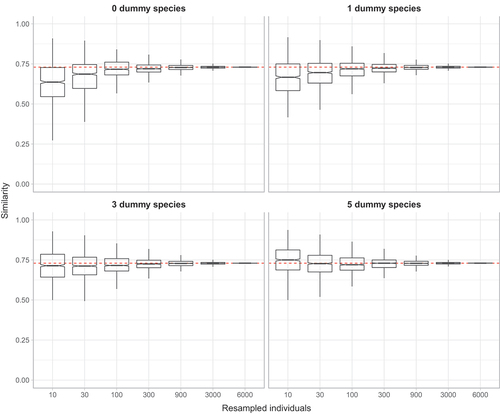
In all datasets tested, undersampling generally led to underestimates of assemblage similarities and adding dummy species resulted in a decrease in the severity of underestimations, with larger numbers of dummy species resulting in less severe underestimates. In Figure 1 we provide the dataset Muturi et al. (2006) as an example. The other cases are reported in Online Resource 2.

Figure 1. Similarity boxplot of Muturi et al. (2006) dataset for random sub-samples of 10, 30, 100, 300, 900, 3000, 6000 individuals. The red dashed line indicates the similarity value calculated when considering the complete dataset. The plots for the other datasets are presented in the Online Resource 2.

When considering all datasets, dummy species also contributed to increase the precision level, and led to a reduction in the erratic behaviour of estimations, and this effect was more pronounced with small sample sizes for which the Levene’s test for equality of variances revealed significant heterogeneity (P < 0.05) (Figure 2, Table II).

Figure 2. Barplot of mean variance ± SE of similarity for random sub-samples of 10, 30, 100, 300, 900, 3000, 6000 individuals obtained adding zero, one, three or five dummy species.

Table II. P-values of Levene’s test obtained by comparing variances estimated adding zero, one, three or five dummy species at different numbers of individuals drawn from the original dataset.

	Resampled individuals
Paper dataset	10	30	100	300	900	3000	6000
Andresen (2003)	<0.0001	0.054	0.465	0.394	0.667	–	–
Bonham et al. (2002)	<0.0001	<0.0001	0.280	0.935	0.538	–	–
Boulton et al. (2005)	<0.0001	0.001	0.020	0.427	0.560	–	–
Collier et al. (1997)	<0.0001	0.522	0.759	0.221	–	–	–
Gristina et al. (2006)	0.004	0.210	0.416	0.704	0.850	0.595	–
Hardersen et al. (2014)	<0.0001	0.001	0.012	0.127	0.173	–	–
Heck et al. (1995)	<0.0001	0.091	0.301	0.304	0.646	0.976	–
Horváth et al. (2013)	<0.0001	0.010	0.021	0.777	0.487	–	–
Jokimäki and Kaisanlahti-Jokimäki (2003)	<0.0001	0.017	0.798	0.289	–	–	–
Maes et al. (2016)	<0.0001	<0.0001	0.467	0.543	0.212	0.956	0.914
Mueter and Norcross (2000)	<0.0001	0.140	0.328	0.991	0.033	–	–
Muturi et al. (2006)	<0.0001	<0.0001	0.110	0.662	0.275	0.210	0.837
Niemelä et al. (2002)	<0.0001	0.001	0.413	0.327	0.813	–	–
Shah et al. (2003)	<0.0001	<0.0001	0.771	0.377	0.220	0.379	0.667
Stark et al. (2003)	<0.0001	0.002	0.398	0.775	0.538	0.911	–
Thorn et al. (2014)	<0.0001	0.003	0.151	0.060	0.644	0.722	0.477

As expected, the simulations resulted in mean values of the relative Good-Turing coverage of detected species which increased with larger numbers of resampled individuals, ranging from 77% ± 18% for sub-samples with 10 individuals, corresponding to a mean coverage deficit of 23%, to 100% ± 0.00% for those with 6000 individuals (coverage deficit 0%) (Table III).

Table III. Mean values (±sd) of Good-Turing sample completeness at the increasing number of individuals resampled from the species of the original dataset.

	Resampled individuals
Assemblage column in each dataset (cf. Table I)	10	30	100	300	900	3000	6000
Assemblage 1	0.78 ± 0.17	0.88 ± 0.10	0.95 ± 0.05	0.98 ± 0.03	0.99 ± 0.01	1.00 ± 0.00	1.00 ± 0.00
Assemblage 2	0.77 ± 0.18	0.89 ± 0.10	0.95 ± 0.06	0.98 ± 0.03	0.99 ± 0.01	1.00 ± 0.00	1.00 ± 0.00

(-) Values could not be calculated.

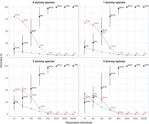
Combining the results from all selected studies showed that with a sample of 10 individuals an underestimation occurred in 80% of the cases, while the values were close to the true Bray–Curtis (±10%) only in 13.2% of cases. Adding dummy species to the assemblages leads to less frequent underestimations resulting in 67.3% of estimates falling below the 10% limit with one dummy species and 48.5% with three dummy species. With five dummy species overestimates became more frequent than underestimates, and the latter were observed in 35% of cases. Increasing the numbers of sampled individuals resulted in higher levels of accuracy of the estimated similarities and in less underestimates. For example, drawing 100 individuals from the complete dataset resulted in 47% of the values to fall within ±10% of the similarity value of the complete dataset. The addition of three or five dummy species increased these values to 52.4% and 54.3%, respectively, and the frequencies of underestimates was reduced to 36.3% and 30.8% respectively. However, to reach an accuracy above 95%, more than 900 individuals needed to be sampled and these returned Bray–Curtis values that on average resulted in under- and over-estimation rates below 2%.

It is important to stress the small sample sizes did not only result in poor accuracy but resulted overwhelmingly in the underestimation of the true value. For 10 individuals drawn, the proportion of underestimation rate was 80.3% and only in 6.7% of cases resulted in an overestimation. For 30 individuals sampled, the cases of underestimation were 69.5% while those of overestimation 7.3%. Introducing dummy species evened out the number of over- and under-estimations and at five dummy species both curves started to be comparable (Figure 3).

Figure 3. Accuracy plots, which indicate the proportion of similarity values, calculated for increasing numbers of individuals drawn from the 16 datasets. Black point-ranges represent mean values (±sd) that fall within the range of ±10% around the similarity value calculated with the complete dataset; red dashed lines represent the mean rate of underestimation and blue dashed lines mean rate of overestimation.

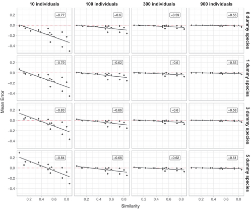
The correlation and regression analyses between the similarity of the assemblages and the mean error are presented in Figure 4. A low number of individuals sampled (e.g. 10) resulted in the highest mean error rates and these were always negative. Interestingly, a clear and statistically significant negative correlation was observed (P < 0.05) in all cases. For 10 individuals drawn, the highest error was observed in assemblages that were most similar and for these underestimates (negative error) was more marked (Figure 4). Increasing the sample size drastically reduced the error and at 900 individuals it was almost zero. Also, increasing the number of dummy species resulted in a reduction of overall error, with 10 sampled individuals and one dummy species negative errors still prevailed and a positive error was only observed for assemblages characterized by a very low similarity. Adding three dummy species to the original dataset resulted in an error which was distributed around zero, with positive small deviations for similarities less than 0.4 and negative numbers for higher values. With five dummy species, the error increased for assemblages with low similarities (i.e. <0.4) and was more evenly distributed around zero. Increasing the sample size to 100, 300 and 900 individuals resulted in a decrease of mean error rates and the effect of adding dummy species decreased. However, even at a sample size of 900 adding three or five dummy species resulted in increased error rates for extreme similarity values (Figure 4).

Figure 4. Mean errors on 16 datasets with an increasing number of (i) resampled individuals (left-right) and (ii) dummy species (top-down). All data are means of 1000 random draws and unbiased estimates have a mean error of zero (indicated by a red dotted line). Correlation coefficients r are reported in labels.

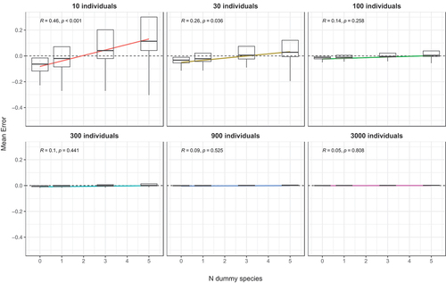
When examining the influence of the number of dummy species on the mean error (Figure 5), it was found that without any dummy species the mean error was negative and increased when adding more dummy species. This increase depended on the number of sampled individuals and this relationship was significant within the range of 10 to 100 individuals. A small number of draws (i.e. 10) resulted in a pronounced positive slope of the regression line, which intercepted 0 at two dummy species. With 100 individuals the slope of the regression was much decreased, and the intercept was observed at five dummy species. However, at 300 individuals the slope was not significantly different from 0 (R = 0.16; P = 0.129).

Figure 5. Boxplot of mean errors with an increasing number of dummy species and regression lines. All data are means of 1000 random draws. Correlation coefficients and P values are reported in labels.

Discussion

Based on actual data, our numerical simulations showed that undersampling generally resulted in underestimates of Bray–Curtis similarities and this finding is in agreement with Chao et al. (2006), Barwell et al. (2015) and Hardersen et al. (2017), and represents an undesirable property because good β diversity metrics should remain constant as the sample size decreases (Barwell et al. 2015). In the datasets tested, underestimates were particularly common for small sample sizes. For instance, similarity estimates based on 10 individuals resulted for 80% of estimates to fall below the ±10% limit around the Bray–Curtis value for the complete dataset. Such individual poor assemblages are not hypothetical but can commonly be found in the literature. To give some examples, the following authors calculated Bray–Curtis similarities for depauperate datasets: Chapman (2002): Some sites with no species; Battaglia et al. (2005): Many sites with fewer than 10 individuals, and some none at all; Stevens and Connolly (2005): Sites with only one or two taxa and very low densities; Luja et al. (2008): Assemblages on average consist of 7 individuals and some transects with zero observations; Chumak et al. (2015): Less than 20 individuals. In all these cases, the similarities calculated were almost certainly negatively biased. Surprisingly, most statistical textbooks do not mention the risk of underestimating Bray–Curtis similarities when only small datasets are available.

For such denuded samples, Clarke et al. (2006) suggested to add a “dummy species” to the original abundance matrix to improve the behaviour of the Bray–Curtis index and we found that this approach alleviated, to some degree, the effect of undersampling on the estimates of similarity. For example, adding one dummy species to samples of 10 individuals led to 13% less underestimates. This result was consistent even for 300 individuals, a sample size considered sufficient for reliable estimates of similarity by Hardersen et al. (2017), and increased accuracy from 80% (no dummy species) to 80.7% (one dummy species). Adding further dummy species to the datasets resulted in less severe underestimates and at five dummy species under- and overestimates were of similar magnitude. However, for small sample sizes, this high number of dummy species resulted in consistent overestimates at low similarity values (Figure 3) and the mean error increased above zero with increasing numbers of dummy species; the trend shown in Figure 5 continued also for seven and nine dummy species (data not shown). Given that the mean error generated by sub-samples should ideally be zero, we suggest that the most appropriate number of dummy species is between 1 and 3 (Figure 5).

Small sample sizes (e.g. 10 individuals) resulted also in highly variable estimates of similarities (Figure 1 and Table II), which is in accordance with the finding by Beck et al. (2013) revealing that undersampling greatly increases random variation in estimates. This is an undesirable property as a good estimator should show little variation (Walther & Moore 2005). However, this behaviour is to be expected as generally the precision of an estimator increases with the square root of the sampling effort (Marriott 1990; Logan 2010). Also in this case, adding dummy species improved the behaviour of estimates, as the variability of estimates decreased, as also shown by Clarke et al. (2006). This improvement was particularly evident for small sample sizes, but still for 30 and 100 individuals the effect was apparent (Figure 4).

The error introduced by undersampling was negatively correlated to the similarity of assemblages. Thus, the more similar two assemblages were, the more likely estimates were underestimated and this tendency was more severe at low sample sizes. We are not aware that this correlation has been reported before. This could have significant consequences in ecological research, where inadequate understanding of how bias, accuracy, and precision influence the estimation of diversity can result in inappropriate selection of estimators, inconsistent estimation outcomes, and suboptimal decision-making. It would be important to test this behaviour of the Bray–Curtis similarity index also with other approaches as it is undesirable. The addition of dummy species resulted in the mean error to be more evenly distributed around zero, but also resulted in more steep regressions of the correlation of similarity against error.

The Bray–Curtis index is widely used in ecological packages in R (e.g. abdiv – Bittinger 2020; ecodist – Goslee & Urban 2007; vegan – Oksanen 2016; wiqid – Meredith 2020) and has been used in at least 1300 scientific papers since 2000 (based on both Scopus and Web of Science abstracts). Moreover, this similarity index is not only applied to directly compare assemblages but is also commonly used to build dissimilarity matrices, which are the basis for further statistics, such as Principal Coordinate Analysis, Permutational Multivariate Analysis of Variance or Nonmetric Multidimensional Scaling (Kindt & Coe 2005; Borcard et al. 2011; Anderson 2017). The fact that similarities are often underestimated and of low precision is likely to compromise the results of these analyses and this becomes more important when only small sample sizes are available. Additional problems stem from datasets comprising high and low similarity values as it is more likely to underestimate similarity values when assemblages are more similar. A further statistical approach that commonly uses Bray–Curtis similarities is the distance–decay plot (Anderson et al. 2011; Wetzel et al. 2012; Filloy et al. 2015; Hardersen et al. 2017). In this case, one undesirable property of the Bray–Curtis similarity index described above leads to more severe underestimates of assemblages that are more similar, resulting in regression lines with a decreased slope. More importantly, more severe underestimates are to be expected when sample sizes are smaller and this tendency is likely to seriously bias the resulting distance decay regression, especially if small and large sample sizes are contained in a single analysis.

Based on our findings, it should be avoided to calculate Bray–Curtis similarities with sample sizes of less than 300 individuals as these are likely to result in underestimates and offer low precision. Reliable estimates can only be computed with datasets which contain more than 300 or 900 individuals and for which the Good-Turing sample completeness resulted approximately 98%; the choice of this minimum sample size depends on what is deemed an acceptable level of precision. This minimum sample size is in the same order of magnitude as the 750–1550 individuals indicated by Schneck and Melo (2010), necessary to adequately estimate resemblance, using the Bray–Curtis index, for macroinvertebrate assemblages in tropical streams.

It is also important to avoid unequal sampling fractions that lead this index to perform erratically (Chao et al. 2006). We also suggest to always add dummy species to the abundance matrix (Clarke et al. 2006) because this results in better and more stable estimates of Bray–Curtis similarities, as underestimates become less likely and precision is increased. As already pointed out by Clarke et al. (2006), differences between the zero-adjusted measure, with a dummy value of 1, and the original Bray–Curtis dissimilarities are slight for samples of counts which contain at least a modest number of individuals. With increasing numbers of individuals sampled, these differences become ever smaller, as is evident from our numerical simulations. It is important to point out that the addition of dummy species alters the resulting Bray–Curtis similarity slightly, but if these are added to all abundance matrices these can validly be compared. The relative values of dissimilarity matter more than their absolute values (Clarke et al. 2006) as most ecologists would be satisfied if dissimilarities of sites in the sample matrix in relation to each other correspond with their relative position derived from complete data (Beck et al. 2013). Similarly, it is often recommended to downweight the contributions of the dominant species by transformation prior to calculating Bray–Curtis similarities (Kindt & Coe 2005; Clarke et al. 2006; Borcard et al. 2011), which also alters the resulting Bray–Curtis similarity.

As shown above, the addition of more dummy species results in less severe underestimates and an increase in precision of the resulting similarity values. At the same time, it increases the negative correlation of the similarity with the mean error and the addition of five dummy species resulted in consistent overestimates at low similarity values. The overestimation of beta diversity is not desirable, as is underestimation. By including an excessive number of dummy species, estimates may be based on artificial and unrealistic conditions, which can result in poor results in ecological research and misinform strategic planning and biodiversity management. Our data seem to indicate that the addition of dummy species to abundance matrices within the range of one to three is a good choice as underestimates of similarities are reduced, precision is increased, and error is more evenly distributed around zero.

Conclusions

In summary, our study shows the importance of considering the error introduced by undersampling on the performance of the Bray–Curtis index and its correlation to the observed similarity when the complete datasets are considered. The results show that undersampling generally resulted in underestimates of assemblage similarities and a possible countermeasure to reduce the severity of this directional bias is the addition of dummy species to the original abundance dataset. This measure is especially important for samples with less than 300 individuals. The Bray–Curtis similarity is frequently employed (Jost et al. 2011; Bacaro et al. 2012), and many textbooks and papers suggest to use this index (e.g. Clarke & Warwick 2001; Kindt & Coe 2005; Schroeder & Jenkins 2018). However, when using this Bray–Curtis similarity, caution is required (Chao et al. 2006; Jost et al. 2011) and by employing sufficiently large sample sizes and adding dummy species, more accurate estimates of beta diversity can be achieved.

Author statement

SH and GLP conceived the ideas, designed methodology, analysed the data and wrote the manuscript. The authors contributed critically to the drafts and gave final approval for publication.

Acknowledgements

We would like to thank Dr. T. Lin Pedersen and the tidyverse community for their precious webinars and online tutorials on the grammar of graphic and tidy packages that made writing the code for this manuscript easier and more effective. S. Hardersen and G. La Porta are grateful to the colleagues from the Centro Nazionale Carabinieri Biodiversità “Bosco Fontana” and the Dipartimento di Chimica, Biologia e Biotecnologie for the positive and stimulating work environment, which allowed to develop the ideas presented. Comments by anonymous reviewers helped to improve the manuscript.

Disclosure statement

No potential conflict of interest was reported by the author(s).

Data availability statement

Source dataset are available in the GitHub repository “bioglp/bc2000.git” (https://github.com/bioglp/bc2000).

Additional information

Funding

This research did not receive any specific grant from funding agencies in the public, commercial, or not-for-profit sectors.

References

- Anderson MJ. 2017. Permutational multivariate analysis of variance (PERMANOVA). In: Balakrishnan N, Colton T, Everitt B, et al., editors. Wiley StatsRef: Statistics reference online. Chichester, UK: John Wiley & Sons, Ltd. pp. 1–15.
- Anderson MJ, Crist TO, Chase JM, Vellend M, Inouye BD, Freestone AL, Sanders NJ, Cornell HV, Comita LS, Davies KF, Harrison SP, Kraft NJB, Stegen JC, Swenson NG. 2011. Navigating the multiple meanings of β diversity: A roadmap for the practicing ecologist. Ecology Letters 14:19–28. DOI: 10.1111/j.1461-0248.2010.01552.x.
- Andresen E. 2003. Effect of forest fragmentation on dung beetle communities and functional consequences for plant regeneration. Ecography 26:87–97. DOI: 10.1034/j.1600-0587.2003.03362.x.
- Bacaro G, Gioria M, Ricotta C. 2012. Testing for differences in beta diversity from plot-to-plot dissimilarities. Ecological Research 27:285–292. DOI: 10.1007/s11284-011-0899-z.
- Barwell LJ, Isaac NJB, Kunin WE. 2015. Measuring β diversity with species abundance data. The Journal of Animal Ecology 84:1112–1122. DOI: 10.1111/1365-2656.12362.
- Battaglia M, Hose GC, Turak E, Warden B. 2005. Depauperate macroinvertebrates in a mine affected stream: Clean water may be the key to recovery. Environmental Pollution 138:132–141. DOI: 10.1016/j.envpol.2005.02.022.
- Beck J, Holloway JD, Schwanghart W. 2013. Undersampling and the measurement of beta diversity. Methods in Ecology and Evolution / British Ecological Society 4:370–382. DOI: 10.1111/2041-210x.12023.
- Beck J, Schwanghart W. 2010. Comparing measures of species diversity from incomplete inventories: An update. Methods in Ecology and Evolution 1:38–44. DOI: 10.1111/j.2041-210X.2009.00003.x.
- Bittinger K. 2020. abdiv: Alpha and beta diversity measures. R package version 0.2.0. Available: https://CRAN.R-project.org/package=abdiv.
- Bloom S. 1981. Similarity indices in community studies: Potential pitfalls. Marine Ecology Progress Series 5:125–128. DOI: 10.3354/meps005125.
- Bonham KJ, Mesibov R, Bashford R. 2002. Diversity and abundance of some ground-dwelling invertebrates in plantation vs. native forests in Tasmania, Australia. Forest Ecology and Management 158:237–247. DOI: 10.1016/S0378-1127(00)00717-9.
- Borcard D, Gillet F, Legendre P. 2011. Numerical ecology with R. New York, NY: Springer Verlag. pp. 306.
- Boulton AM, Davies KF, Ward PS. 2005. Species richness, abundance, and composition of ground-dwelling ants in Northern California grasslands: Role of plants, soil, and grazing. Environmental Entomology 34:96–104. DOI: 10.1603/0046-225X-34.1.96.
- Bray JR, Curtis JT. 1957. An ordination of the upland forest communities of Southern Wisconsin. Ecological Monographs 27:325–349. DOI: 10.2307/1942268.
- Cao Y, Larsen DP, Hughes RM. 2001. Evaluating sampling sufficiency in fish assemblage surveys: A similarity-based approach. Canadian Journal of Fisheries and Aquatic Sciences 58:1782–1793. DOI: 10.1139/f01-120.
- Cardoso P, Borges PAV, Veech JA. 2009. Testing the performance of beta diversity measures based on incidence data: The robustness to undersampling. Diversity & Distributions 15:1081–1090. DOI: 10.1111/j.1472-4642.2009.00607.x.
- Chao A, Chazdon RL, Colwell RK, Shen TJ. 2005. A new statistical approach for assessing similarity of species composition with incidence and abundance data. Ecology Letters 8:148–159. DOI: 10.1111/j.1461-0248.2004.00707.x.
- Chao A, Chazdon RL, Colwell RK, Shen TJ. 2006. Abundance-based similarity indices and their estimation when there are unseen species in samples. Biometrics 62:361–371. DOI: 10.1111/j.1541-0420.2005.00489.x.
- Chao A, Hsieh TC, Chazdon RL, Colwell RK, Gotelli NJ. 2015. Unveiling the species-rank abundance distribution by generalizing the Good-Turing sample coverage theory. Ecology 96:1189–1201. DOI: 10.1890/14-0550.1.
- Chapman MG. 2002. Patterns of spatial and temporal variation of macrofauna under boulders in a sheltered Boulder field. Austral Ecology 27:211–228. DOI: 10.1046/j.1442-9993.2002.01172.x.
- Chumak V, Obrist MK, Moretti M, Duelli P. 2015. Arthropod diversity in pristine vs. managed beech forests in Transcarpathia (Western Ukraine). Global Ecology and Conservation 3:72–82. DOI: 10.1016/j.gecco.2014.11.001.
- Clarke KR, Somerfield PJ, Chapman MG. 2006. On resemblance measures for ecological studies, including taxonomic dissimilarities and a zero-adjusted Bray–Curtis coefficient for denuded assemblages. Journal of Experimental Marine Biology and Ecology 330:55–80. DOI: 10.1016/j.jembe.2005.12.017.
- Clarke KR, Warwick RM. 2001. Change in marine communities: An approach to statistical analysis and interpretation. 2nd ed. Plymouth: PRIMER-E.
- Collier KJ, Smith BJ, Baillie BR. 1997. Summer light‐trap catches of adult Trichoptera in hill‐country catchments of contrasting land use, Waikato, New Zealand. New Zealand Journal of Marine and Freshwater Research 31:623–634. DOI: 10.1080/00288330.1997.9516794.
- Colwell RK, Coddington JA. 1994. Estimating terrestrial biodiversity through extrapolation. Philosophical Transactions of the Royal Society B 311:118–345.
- Filloy J, Grosso S, Bellocq MI. 2015. Urbanization altered latitudinal patterns of bird diversity-environment relationships in the southern Neotropics. Urban Ecosyst 18:777–791. DOI: 10.1007/s11252-014-0429-1.
- Gaston KJ, Spicer JI. 2004. Biodiversity: An introduction. 2nd ed. Malden, USA: Blackwell Publishing. pp. 191.
- Goslee SC, Urban DL. 2007. The ecodist package for dissimilarity-based analysis of ecological data. Journal of Statistical Software 22(7):1–19. DOI: 10.18637/jss.v022.i07.
- Gower JC, Legendre P. 1986. Metric and Euclidean properties of dissimilarity coefficients. Journal of Classification 3:5–48. DOI: 10.1007/BF01896809.
- Gristina M, Bahri T, Fiorentino F, Garofalo G. 2006. Comparison of demersal fish assemblages in three areas of the Strait of Sicily under different trawling pressure. Fisheries Research 81:60–71. DOI: 10.1016/j.fishres.2006.05.010.
- Hardersen S, Corezzola S, Gheza G, Dell’Otto A, La Porta G. 2017. Sampling and comparing odonate assemblages by means of exuviae: Statistical and methodological aspects. Journal of Insect Conservation 21:207–218. DOI: 10.1007/s10841-017-9969-z.
- Hardersen S, Curletti G, Leseigneur L, Platia G, Liberti G, Leo P, Cornacchia P, Gatti E. 2014. Spatio-temporal analysis of beetles from the canopy and ground layer in an Italian lowland forest. Bulletin of Insectology 67:87–97.
- Heck KL, Able KW, Roman CT, Fahay MP. 1995. Composition, abundance, biomass, and production of macrofauna in a New England estuary: Comparisons among eelgrass meadows and other nursery habitats. Estuaries 18:379. DOI: 10.2307/1352320.
- Horváth B, Tóth V, Kovács G. 2013. The effect of herb layer on nocturnal Macrolepidoptera (Lepidoptera: Macroheterocera) communities. Acta Silvatica et Lignaria Hungarica 9:43–56. DOI: 10.2478/aslh-2013-0004.
- Jokimäki J, Kaisanlahti-Jokimäki ML. 2003. Spatial similarity of urban bird communities: A multiscale approach. Journal of Biogeography 30:1183–1193. DOI: 10.1046/j.1365-2699.2003.00896.x.
- Jost L, Chao A, Chazdon RL. 2011. Compositional similarity and β (beta) diversity. In: Magurran AE, McGill BJ, editors. Biological diversity – Frontiers in measurement and assessment. Oxford: Oxfard University Press. pp. 66–84.
- Jurasinski G, Retzer V, Beierkuhnlein C. 2009. Inventory, differentiation, and proportional diversity: A consistent terminology for quantifying species diversity. Oecologia 159:15–26. DOI: 10.1007/s00442-008-1190-z.
- Kindt R, Coe R. 2005. Tree diversity analysis. A manual and software for common statistical methods for ecological and biodiversity studies. Nairobi: World Agroforestry Centre (ICRAF). pp. 196.
- Legendre P, De Cáceres M. 2013. Beta diversity as the variance of community data: Dissimilarity coefficients and partitioning. Ecology Letters 16:951–963. DOI: 10.1111/ele.12141.
- Legendre P, Gallagher ED. 2001. Ecologically meaningful transformations for ordination of species data. Oecologia 129:271–280. DOI: 10.1007/s004420100716.
- Logan M. 2010. Biostatistical design and analysis using R: A practical guide. Chichester, West Sussex: Wiley-Blackwell. pp. 546.
- Luja VH, Herrando-Pérez S, González-Solís D, Luiselli L. 2008. Secondary rain forests are not havens for reptile species in tropical Mexico. Biotropica 40:747–757. DOI: 10.1111/j.1744-7429.2008.00439.x.
- Maes D, Vanreusel W, Herremans M, Vantieghem P, Brosens D, Gielen K, Beck O, Van Dyck H, Desmet P, Natuurpunt V. 2016. A database on the distribution of butterflies (Lepidoptera) in northern Belgium (Flanders and the Brussels Capital Region). ZooKeys 585:143–156. DOI: 10.3897/zookeys.585.8019.
- Magurran AE. 2004. Measuring biological diversity. Malden, USA: Blackwell Publishing. pp. 256.
- Marriott FHC. 1990. A dictionary of statistical terms. 5th ed. Harlow, Essex: Longman Publishing Group. pp. 223.
- Melo AS. 2021. Heavy-weighting rare species in dissimilarity indices improve recovery of multivariate groups. Ecological Complexity 46:100925. DOI: 10.1016/j.ecocom.2021.100925.
- Meredith M. 2020. wiqid: Quick and dirty estimates for wildlife populations. R package version 0.2.3. Available: https://CRAN.R-project.org/package=wiqid.
- Minchin PR. 1987. An evaluation of the relative robustness of techniques for ecological ordination. Vegetatio 69:89–107. DOI: 10.1007/BF00038690.
- Mueter FJ, Norcross BL. 2000. Species composition and abundance of juvenile groundfishes around Steller Sea Lion Eumetopias jubatus rookeries in the Gulf of Alaska. Alaska Fishery Research Bulletin 7:33–43.
- Muturi EJ, Shililu J, Jacob B, Gu W, Githure J, Novak R. 2006. Mosquito species diversity and abundance in relation to land use in a riceland agroecosystem in Mwea, Kenya. Journal of Vector Ecology 31:129–137. DOI: 10.3376/1081-1710(2006)31[129:MSDAAI]2.0.CO;2.
- Niemelä J, Kotze DJ, Venn S, Penev L, Stoyanov I, Spence J, Hartley D, De Oca EM. 2002. Carabid beetle assemblages (Coleoptera, Carabidae) across urban-rural gradients: An international comparison. Landscape Ecology 17:387–401. DOI: 10.1023/A:1021270121630.
- Oksanen J. 2016. Multivariate analysis of ecological communities in R: Vegan tutorial. Available: http://cc.oulu.fi/~jarioksa/opetus/metodi/vegantutor.pdf.
- Oksanen J, Blanchet FG, Friendly M, Kindt R, Legendre P, McGlinn D, Minchin PR, O’Hara RB, Simpson GL, Solymos P, Stevens MHH, Szoecs E, Wagner H. 2019. Package vegan: Community ecology package. Version 2(5–6):296.
- Pruim RD, Kaplan T, J Horton NJ. 2017. The mosaic package: Helping students to ‘Think with data’ using R. The R Journal 9(1):77–102. DOI: 10.32614/RJ-2017-024.
- R Core Team. 2022. R: A language and environment for statistical computing. Vienna, Austria: R Foundation for Statistical Computing. Available: https://www.R-project.org/.
- Ricotta C, Podani J. 2017. On some properties of the Bray-Curtis dissimilarity and their ecological meaning. Ecological Complexity 31:201–205. DOI: 10.1016/j.ecocom.2017.07.003.
- Schmera D, Eros T. 2006. Estimating sample representativeness in a survey of stream caddisfly fauna. Annales de Limnologie-International Journal of Limnology 42(3):181–187. DOI: 10.1051/limn/2006019.
- Schneck F, Melo AS. 2010. Reliable sample sizes for estimating similarity among macroinvertebrate assemblages in tropical streams. Annales de Limnologie-International Journal of Limnology 46(2):93–100. DOI: 10.1051/limn/2010013.
- Schroeder PJ, Jenkins DG. 2018. How robust are popular beta diversity indices to sampling error. Ecosphere 9:1–14. DOI: 10.1002/ecs2.2100.
- Shah PA, Brooks DR, Ashby JE, Perry JN, Woiwod IP. 2003. Diversity and abundance of the coleopteran fauna from organic and conventional management systems in southern England. Forest Agriculture Enterprises 5:51–60. DOI: 10.1046/j.1461-9563.2003.00162.x.
- Stark JS, Riddle MJ, Simpson RD. 2003. Human impacts in soft-sediment assemblages at Casey Station, East Antarctica: Spatial variation, taxonomic resolution and data transformation. Austral Ecology 28:287–304. DOI: 10.1046/j.1442-9993.2003.01289.x.
- Stevens T, Connolly RM. 2005. Local-scale mapping of benthic habitats to assess representation in a marine protected area. Marine and Freshwater Research 56:111. DOI: 10.1071/MF04233.
- Thorn S, Bässler C, Gottschalk T, Hothorn T, Bussler H, Raffa K, Müller J. 2014. New insights into the consequences of post-windthrow salvage logging revealed by functional structure of saproxylic beetles assemblages. PLoS ONE 9:7. DOI: 10.1371/journal.pone.0101757.
- Walther BA, Moore JL. 2005. The concepts of bias, precision and accuracy, and their use in testing the performance of species richness estimators, with a literature review of estimator performance. Ecography 28:815–829. DOI: 10.1111/j.2005.0906-7590.04112.x.
- Wetzel CE, Bicudo DDC, Ector L, Lobo EA, Soininen J, Landeiro VL, Bini LM. 2012. Distance decay of similarity in neotropical diatom communities. PLoS ONE 7:e45071. DOI: 10.1371/journal.pone.0045071.
- Wickham H. 2016. ggplot2: Elegant graphics for data analysis. New York: Springer-Verlag.
- Zou Y, Axmacher JC. 2019. The Chord-Normalized Expected Species Shared (CNESS)-Distance represents a superior measure of species turnover patterns. Methods in Ecology and Evolution / British Ecological Society 11:273–280. DOI: 10.1111/2041-210X.13333.