Speeding up Composite Differential Evolution for structural optimization using neural networks

ABSTRACT

Composite Differential Evolution (CoDE) is categorized as a (µ + λ)-Evolutionary Algorithm where each parent produces three trials. Thanks to that, the CoDE algorithm has a strong search capacity. However, the production of many offspring increases the computation cost of fitness evaluation. To overcome this problem, neural networks, a powerful machine learning algorithm, are used as surrogate models for rapidly evaluating the fitness of candidates, thereby speeding up the CoDE algorithm. More specifically, in the first phase, the CoDE algorithm is implemented as usual, but the fitnesses of produced candidates are saved to the database. Once a sufficient amount of data has been collected, a neural network is developed to predict the constraint violation degree of candidates. Offspring produced later will be evaluated using the trained neural network and only the best among them is compared with its parent by exact fitness evaluation. In this way, the number of exact fitness evaluations is significantly reduced. The proposed method is applied for three benchmark problems of 10-bar truss, 25-bar truss, and 72-bar truss. The results show that the proposed method reduces the computation cost by approximately 60%.

KEYWORDS:

• Structural optimization
• composite differential evolution
• machine learning
• surrogate model
• neural network

1. Introduction

Structural optimization (SO) plays an important role in the field of architecture, engineering, and construction. Applying SO in the design phase not only reduces the construction cost but also saves the consumption of natural resources, thereby minimizing the impact on the environment. Therefore, SO has gained great attention in recent years. SO is a kind of constrained optimization problem, in which the final solution must satisfy a set of design constraints. Checking design constraints is often computationally expensive because it requires conducting finite element analysis. In the past three decades, evolutionary algorithms have been preferred for this task due to their capability to cope with the multimodal objective function as well as nonlinear constraints. Many evolutionary algorithms have been used to optimize structures, for example, GA (Rajeev & Krishnamoorthy, 1992), ES (Cai & Thierauf, 1996), DE (Wang et al., 2009). Particularly, many researchers have selected the DE algorithm for solving structural optimization because it is simple and easy to implement.

Basically, DE has four operators: initialization, mutation, crossover, and selection, in which the mutation operator strongly affects the performance of the DE algorithm. There exist many mutation strategies, for example, ‘rand/1’, ‘rand/2’, ‘best/1’, ‘best/2’, ‘current-to-rand/1’, and ‘current-to-best/1’, and each of them has its own advantage. The ‘rand/1’ strategy is strong in exploring new space but it is weak in the local exploitation. Consequently, the convergence speed of the ‘rand/1’ strategy is very slow. On the contrary, the ‘current-to-best/1’ has a strong exploitation capacity but it is easy to fall local optimum. It is noted that the balance of the global exploration and the local exploitation is the key factor to ensure the performance of a metaheuristic algorithm. Some techniques have been introduced for this purpose. For instance, the ‘current-to-pbest’ mutation strategy was presented by Zhang and Sanderson (2009), in which the best vector x_best at the current generation in the ‘current-to-best’ strategy is replaced by the vector x_pbest randomly selected from the top p × NP individuals. This mutation strategy is able to avoid trapping to a local optimum. This idea was then applied in the Adaptive DE algorithm when optimizing truss structures (Bureerat & Pholdee, 2016). Another technique, called ‘opposition-based mutation’ was introduced by Rahnamayan et al. (2008) to ensure that the difference is always oriented towards the better vector. The opposition-based mutation was then employed for solving truss structure optimization problems (Pham, 2016). Furthermore, it can be observed that in the sooner generations, the diversity of the population plays an important role while the ability of the local exploitation is needed in the later generations. Thus, an adaptive mutation scheme was proposed (Ho-Huu et al., 2016) where one of two mutation strategies ‘rand/1’ and ‘current-to-best/1’ is adaptively selected during the optimization process.

Another approach is to use multiple mutation strategies simultaneously with the aim of balancing global exploration and local exploitation. Mallipeddi et al. (2011) developed the EPSDE algorithm, in which three strategies ‘best/2’, ‘rand/1’, ‘current-to-rand/1’ are selected to form a pool. The scaling factor F varies from 0.4–0.9 with the step of 0.1 and the crossover rate Cr is taken a value from the list of (0.1–0.9) with the step of 0.1. Initially, each target vector in the initial population is associated with a mutation strategy and a control parameter setting from the pools. If the trial vector is better than the target vector, the trial vector is kept to the next generation and the combination of the current mutation strategy and parameters are saved into the memory. Otherwise, a new trial vector is produced using a new combination of mutation strategy and control parameters from pools or the memory. In this way, the probability of producing offspring which is better than its parent gradually increases during the evolution.

Wang and Cai (2011) proposed the (µ + λ)-Constrained Differential Evolution ((µ + λ)-CDE) in which three mutation strategies (i.e. ‘rand/1’, ‘rand/2’, and ‘current-to-best/1’) are used simultaneously to solve constrained optimization problems. The experimental results show that the (µ + λ)-CDE algorithm is very competitive when it outperformed other algorithms in benchmark functions. This algorithm was later improved into the (µ + λ)-ICDE (Jia et al., 2013). In this study, a new proposed mutation strategy called ‘current-to-rand/best/1’ was used instead of the ‘current-to-best/1’ strategy.

In both studies above, three offspring are generated by using three different mutation strategies but the scaling factor and the crossover rate are fixed during the optimization process. Obviously, these parameters also strongly influence the performance of the algorithm. A large value of the scaling factor F increases the population diversity over the design space while a small value of F speeds up the convergence. The influence of the crossover rate Cr is similar. Based on this observation, Wang et al. (2011) proposed a new algorithm called Differential Evolution with composite trials and control parameters (CoDE) for solving unconstrained optimization problems. In details, the mutation strategies including ‘rand/1/bin’, ‘rand/2/bin’, and ‘current-to-rand/1’ and three pairs of control parameters [F = 1.0, Cr = 0.1], [F = 1.0, Cr = 0.9], [F = 0.8, Cr = 0.2] are randomly combined to generate three trial vectors. The tests on 25 benchmark functions proposed in the CEC 2005 show that CoDE is better than seven algorithms including JADE, jDE, SaDE, EPSDE, CLPSO, CMA-ES, and GL-25. Following this trend, the C²oDE is developed for constrained optimization problems (Wang et al., 2019). Three strategies used in the C²oDE include ‘current-to-rand/1’, modified ‘rand-to-best/1/bin’, and ‘current-to-best/1/bin’. Additionally, at each generation, the scaling factor and the crossover rate are randomly selected a value from the pool F_pool = [0.6, 0.8, 1.0] and Cr_pool = [0.1, 0.2, 1.0], respectively. The C²oDE is proved to be as good as or better than other state-of-the-art algorithms.

Although these above modifications greatly improve the efficiency of the DE, the computation time is also increased by approximately three times due to the expansion of the population. For problems where the fitness evaluation is very costly, for example, structural optimization, the use of the C²oDE is not beneficial. In recent years, machine learning (ML) has been increasingly applied in the field of structural engineering. The results of some previous studies have shown that ML can accurately predict the behaviour of structures (Kim et al., 2020; Nguyen & Vu, 2021; Truong et al., 2020). This leads to a potential solution to reduce the computation cost of the composite DE. In fact, despite generating three trial vectors, only the best of them is used to compare with their parent vector. By building ML-based surrogate models to identify the best trial vector, the number of exact fitness evaluations can be greatly reduced and the overall computation time is consequently shortened.

In the literature, there exist a few studies relating to this topic. Mallipeddi and Lee (2012) employed a Kriging model to improve the performance of EPSDE. The Kriging surrogate model was utilized with the aim of generating a competitive trial vector with less computational cost. Krempser et al. (2012) generated three trial vectors using ‘best/1/bin’, ‘target-to-best/1/bin’ and ‘target-to-rand/1/bin’, then a Nearest Neighbors-based surrogate model was used to detect the best one. The advantage of the Nearest Neighbors algorithm is that it does not require the training process as other machine learning algorithms, thus, data is always updated. Although there exist many ML algorithms, the comparative study indicates that neural networks are a good choice for regression tasks due to a trade-off between accuracy and computation cost (Nguyen & Vu, 2021). In the study presented at the 12th international conference on computational collective intelligence (ICCCI 2020) (Nguyen & Vu, 2020), surrogate models developed based on neural networks are integrated into the DE algorithm to reduce the optimization time. However, due to the error of the surrogate model, the optimal results found by the surrogate assisted DE algorithm and the conventional DE algorithm always have a little difference.

This paper is an extended version of the ICCCI 2020 paper. In this work, neural networks do not directly replace the exact fitness evaluation. Alternately, neural networks are trained to predict the constraint violation degree of trial vectors. The trial vector having the smallest predicted value is then selected for the knockout selection with the target vector. The final selection is still based on the exact fitness evaluation, thus ensuring to find the true optimum. The proposed approach takes full advantage of the CoDE algorithm but it still keeps the optimization time as fast as the conventional DE algorithm.

The rest of the paper is organized as follows. Section 2 states the optimization problem for truss structures and the basics of the CoDE algorithm. Neural networks are briefly presented in Section 3. The proposed approach is introduced in Section 4. Three test problems are carried out in Section 5 to demonstrate the efficiency of the proposed approach. Section 6 concludes this paper.

2. Structural optimization using Composite Differential Evolution

2.1. Optimization of truss structures

In this study, the proposed approach is employed in minimizing the weight of truss structures but it can be used for optimizing all kinds of structures. The optimal weight design of a truss structure is presented below.

Find a set of cross-sectional areas of truss members A = [A₁, A₂, … , A_i, … , A_n] where A_i^L ≤ A_i ≤ A_i^U to minimize the weight of the structure: (1) $W\left(\mathit{A}\right)=\sum _{i=1}^n{\rho }_i{A}_i{l}_i$(1) subject to design constraints: (2) $\{\begin{array}{c}{g}_i^s=\left|{\displaystyle \frac{{\sigma }_i}{{\sigma }_{\mathrm{a}\mathrm{l}\mathrm{l}\mathrm{o}\mathrm{w}}}}\right|-1\le 0,i=1,2,\dots ,n\\ g_j^{\mathrm{d}\mathrm{i}\mathrm{s}\mathrm{p}}=\left|{\displaystyle \frac{{\delta }_j}{{\delta }_{\mathrm{a}\mathrm{l}\mathrm{l}\mathrm{o}\mathrm{w}}}}\right|-1\le 0,j=1,2,\dots ,m\end{array}$(2) where: A_i is the cross-sectional area of the ith member; A_i^L and A_i^U are the lower bound and the upper bound of the cross-sectional area of the ith member; ρ_i and l_i are the density and the length of the ith member, respectively; σ_i and ${\sigma }_j^{\mathrm{a}\mathrm{l}\mathrm{l}\mathrm{o}\mathrm{w}}$ are the calculated stress and the allowable stress of ith member, respectively; δ_j and ${\delta }_j^{\mathrm{a}\mathrm{l}\mathrm{l}\mathrm{o}\mathrm{w}}$ are the calculated displacement and the allowable displacement of jth node, respectively; n is the number of truss members; and m is the number of free nodes.

2.2. Composite Differential Evolution for constrained optimization problems

2.2.1. Basic DE

DE was designed by Storn and Price (1997). In general, DE contains four steps: initialization, mutation, crossover, and selection.

Firstly, an initial population of NP target vectors {x₁⁽⁰⁾, x₂⁽⁰⁾, … , x_NP⁽⁰⁾} is randomly generated over the design space. Each target vector contains D components x_i⁽⁰⁾ = {x_i,1⁽⁰⁾, x_i,2⁽⁰⁾, … , x_i,D⁽⁰⁾}. NP is the population size, D is the number of design variables, and x_i,j⁽⁰⁾ is the jth component of the ith vector. At generation t, each target vector produces a mutant vector using the mutation operator. Some widely used mutation operators are presented as follows. (3a) $\mathrm{r}\mathrm{a}\mathrm{n}\mathrm{d}/1{\mathit{v}}_i^{\left(t\right)}={\mathit{x}}_{r1}^{\left(t\right)}+F\times \left({\mathit{x}}_{r2}^{\left(t\right)}-{\mathit{x}}_{r3}^{\left(t\right)}\right)$(3a) (3b) $\mathrm{r}\mathrm{a}\mathrm{n}\mathrm{d}/2{\mathit{v}}_i^{\left(t\right)}={\mathit{x}}_{r1}^{\left(t\right)}+F\times \left({\mathit{x}}_{r2}^{\left(t\right)}-{\mathit{x}}_{r3}^{\left(t\right)}\right)+F\times \left({\mathit{x}}_{r4}^{\left(t\right)}-{\mathit{x}}_{r5}^{\left(t\right)}\right)$(3b) (3c) $\mathrm{b}\mathrm{e}\mathrm{s}\mathrm{t}/1{\mathit{v}}_i^{\left(t\right)}={\mathit{x}}_{best}^{\left(t\right)}+F\times \left({\mathit{x}}_{r1}^{\left(t\right)}-{\mathit{x}}_{r2}^{\left(t\right)}\right)$(3c) (3d) $\mathrm{b}\mathrm{e}\mathrm{s}\mathrm{t}/2{\mathit{v}}_i^{\left(t\right)}={\mathit{x}}_{best}^{\left(t\right)}+F\times \left({\mathit{x}}_{r1}^{\left(t\right)}-{\mathit{x}}_{r2}^{\left(t\right)}\right)+F\times \left({\mathit{x}}_{r3}^{\left(t\right)}-{\mathit{x}}_{r4}^{\left(t\right)}\right)$(3d) (3e) $\mathrm{c}\mathrm{u}\mathrm{r}\mathrm{r}\mathrm{e}\mathrm{n}\mathrm{t}\text{-}\mathrm{t}\mathrm{o}\text{-}\mathrm{b}\mathrm{e}\mathrm{s}\mathrm{t}/1{\mathit{v}}_i^{\left(t\right)}={\mathit{x}}_i^{\left(t\right)}+F\times \left({\mathit{x}}_{best}^{\left(t\right)}-{\mathit{x}}_i^{\left(t\right)}\right)+F\times \left({\mathit{x}}_{r1}^{\left(t\right)}-{\mathit{x}}_{r2}^{\left(t\right)}\right)$(3e) where: x_i^(t) is the target vector; v_i^(t) is the mutant vector; x_r1^(t), x_r2^(t), x_r3^(t), x_r4^(t), x_r5^(t) are vectors which are randomly selected from the population; F is the scaling factor; x_best^(t) is the best target vector of the population at generation t.

Then, a binomial crossover operator is employed to produce a trial vector as follows: (4) $u_{i,j}^{\left(t\right)}=\{\begin{array}{c}{v}_{i,j}^{\left(t\right)}\mathrm{i}\mathrm{f}j=K\mathrm{o}\mathrm{r}\mathrm{r}\mathrm{a}\mathrm{n}\mathrm{d}\left[0,1\right]\le Cr\\ x_{i,j}^{\left(t\right)}\mathrm{o}\mathrm{t}\mathrm{h}\mathrm{e}\mathrm{r}\mathrm{w}\mathrm{i}\mathrm{s}\mathrm{e}\end{array}$(4) where: u_i,j^(t), v_i,j^(t), x_i,j^(t) are the jth component of the trial vector, the mutant vector, and the target vector, respectively; K is an integer randomly selected from 1 to D; rand[0,1] is a uniformly distributed random number on the interval [0,1]; Cr is the crossover rate.

Next, the trial vector u_i^(t) and the target vector x_i^(t) are compared, and the better one is kept for the (t + 1)th generation. The cycle of three steps (i.e. mutation, crossover, and selection) is performed repeatedly until the stopping condition is reached.

2.2.2. Composite DE

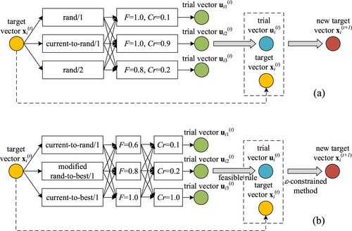
CoDE was proposed by Wang et al. (2011) for unconstrained optimization problems. The basic idea behind the CoDE is to randomly combine three mutation strategies with three pairs of F and Cr for producing three trial vectors. Three mutation strategies used in the CoDE are ‘rand/1/bin’, ‘rand/2/bin’, and ‘current-to-rand/1’. Three fixed control parameter settings are [F = 1.0, Cr = 0.1], [F = 1.0, Cr = 0.9], [F = 0.8, Cr = 0.2]. Through experimental results, the CoDE achieves outstanding performance.

A variation of Composite DE for constrained optimization problems called C²oDE was introduced in 2018 (Wang et al., 2019). Some modifications in the C²oDE can be summarized as follows. First of all, three mutation strategies used in C²oDE are: ‘current-to-rand/1’, ‘current-to-best/1/bin’, and modified ‘rand-to-best/1/bin’. This modification improves the trade-off between diversity and convergence when searching over design space.

The second difference is that in the C²oDE, the scaling factor F and the crossover rate Cr are taken from two pools F_pool and Cr_pool, respectively. According to the authors’ recommendation, the scaling factor pool consists of three values F_pool = [0.6,0.8,1.0] while the crossover rate pool also contains three values Cr_pool = [0.1,0.2,1.0].

The final modification is carried out in the selection step. Obviously, the balance between minimizing the degree of constraint violation and minimizing the objective function is very important in constrained optimization problems. Therefore, the authors employ two constraint handling techniques simultaneously. The feasible rule proposed by Deb (2000) is utilized to select the best trial vector among three ones while the selection between the best trial vector and the target vector is based on the ϵ-constrained method (Takahama, 2006). The details of the feasible rule and the ϵ-constrained method are presented in Section 2.3. Additionally, a brief illustration of the CoDE and the C²oDE is displayed in Figure 1.

Figure 1. Illustration of CoDE and C²oDE. (a) CoDE, (b) C²oDE.

2.3. Constraint handling technique

Generally, most optimization algorithms are designed to solve unconstrained problems. These algorithms can be also applied to constrained problems by using constraint handling techniques, for example, penalty function, feasible rule, or ϵ-constrained method.

The most widely used constraint handling technique is the penalty method in which a term is added to the objective function as a penalty. (5) $F\left(\mathit{x}\right)=f\left(\mathit{x}\right)+p\left(\mathit{x}\right)$(5) where: F(x) is the fitness function, f(x) is the objective function; p(x) is the penalty function. The penalty function p(x) is larger than zero when any design constraint is violated and is zero when all constraints are satisfied.

An effective method to handle constrained optimization problems is the feasible rules proposed by Deb (2000). According to Deb's rules, in a pairwise comparison, the better solution is chosen based on three criteria as follows.

• Any feasible solution is preferred to any infeasible solution.

• Among two feasible solutions, the one having lower objective function value is preferred.

• Among two infeasible solutions, the one having smaller constraint violation is preferred.

It can be seen that in Deb's rule, the satisfaction of constraints is the first priority, followed by the minimization of the objective function. Takahama et al. (2006) proposed the ϵ-constrained method as follows.

In the ϵ-constrained method, the constraint violation ϕ(x) is defined as the maximum of all constraints or the sum of all constraints. (6a) $\varphi \left(\mathit{x}\right)=max\left\{{max}_j\left\{0,g_j\left(\mathit{x}\right)\right\}\right\}$(6a) (6b) $\varphi \left(\mathit{x}\right)=\sum _j{\Vert max\left\{0,g_j\left(\mathit{x}\right)\right\}\Vert }^p$(6b) where: p is a positive number.

The point x₁ is assumed to be better than the point x₂ when (7) ${\mathit{x}}_1{\le }_{ϵ}{\mathit{x}}_2\iff \{\begin{array}{c}{f}_1\le f_2,\mathrm{i}\mathrm{f}{\varphi }_1,{\varphi }_2\le ϵ\\ f_1\le f_2,\mathrm{i}\mathrm{f}{\varphi }_1={\varphi }_2\\ {\varphi }_1<{\varphi }_2,\mathrm{o}\mathrm{t}\mathrm{h}\mathrm{e}\mathrm{r}\mathrm{w}\mathrm{i}\mathrm{s}\mathrm{e}\end{array}$(7) in which: f₁, ϕ₁ are the objective function and the constraint violation of the point x₁, respectively; f₂, ϕ₂ are the objective function and the constraint violation of the point x₂, respectively.

The comparison described in Eq. (7) is called the ϵ-level comparison. Where the ϵ value is equal to infinity, two points x₁ and x₂ are compared in terms of the objective function values. In contrast, if ϵ equals 0, the ϵ-level comparison becomes Deb's rules.

3. Brief introduction to artificial neural network

Artificial neural network (ANN) is known as one of the most powerful computational paradigms. This model was first designed in 1958 based on the understanding of the human brain's structure (Rosenblatt, 1958). In biological brains, there are billions of neurons connected to each other through synapses. The role of synapses is to transmit the electrical signal to other neurons. Similarly, ANNs are composed of nodes that simulate neurons and connections that imitate the synapses of the brain. An artificial neuron receives inputs from previous neurons, transforms them by the activation function, and sends them to the following neurons via connections. Each connection is assigned a weight to represent the magnitude of the signal. The activation function attached to artificial neurons is frequently nonlinear, allowing ANNs to capture complex data. Until now, many architectures of ANN have been introduced, for example, feed-forward neural networks (FFNN), convolution neural networks (CNN), recurrent neural networks (RNN), etc. Each architecture of ANNs is designed for a specific task. CNN is primarily used for tasks related to image processing, and RNN is suitable for time series data. In the field of structural engineering, FFNN is commonly used.

In FFNN, neurons are organized into many layers including the input layer, the hidden layers, and the output layers. The information moves through the FFNN in a one-way direction from the input layer through hidden layers to the output layers. The simplest kind of FFNN is a ‘single-layer perceptron’ which contains only one hidden layer. Neural networks having more than one hidden layer are called ‘multilayer perceptron’ or ‘deep neural networks’ with the aim of improving the performance of the models. A typical architecture of a deep neural network is shown in Figure 2.

Figure 2. Typical architecture of Feed-Forward Neural Networks.

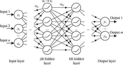
It can be expressed as follows. The neuron of jth layer u_j (j = 1,2, … ,J) receives a sum of input x_i (i = 1,2, … ,I) which is multiplied by the weight w_ji and will be transformed into the input of the neuron in the next layer: (8) $x_j=f\left(u_j\right)=f\left(\sum _{i=1}^I{w}_{ji}{x}_i\right)$(8) where f(.) is the activation function. The most commonly used activation functions are: tanh, sigmoid, softplus, and rectifier linear unit (ReLU).

The loss function is used to measure the error between predicted values and true values. The loss function is chosen depending on the type of task. For regression tasks, the loss functions can be Mean Squared Error (MSE), Mean Absolute Error (MAE), or Root Mean Squared Error (RMSE). To adapt NN for better predictions, the network must be trained. The training process is essentially finding a set of weights in order to minimize the loss function. In other words, it is an optimization process. In the field of machine learning, the commonly used optimization algorithms are stochastic gradient descent (SGD) or Adam optimizer. An effective technique, namely ‘backpropagation’, developed by Rumelhart et al. (1986) is normally used for training, in which weights can be updated with the gradient descent method as follows: (9) $w_{ij}^{(t+1)}=w_{ij}^{\left(t\right)}-\eta {\displaystyle \frac{\mathrm{\partial }E}{\mathrm{\partial }{w}_{ij}^{\left(t\right)}}}$(9) where: E is the loss function between the predicted and the true values; η is the learning rate.

4. Proposed approach

The proposed approach, called surrogate assisted-CoDE (SA-CoDE), is presented in Figure 3, in which the optimization process is separated into two phases.

Figure 3. Workflow of surrogate assisted Composite Differential Evolution (SA-CoDE).

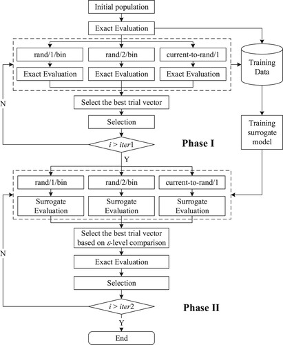
In the first phase, the CoDE algorithm is implemented as usual. All trial vectors produced in this phase are checked design constraints. All information including details of trial vectors as well as their constraint violation degrees is saved into memory. Data collected during this phase are then used to train a neural network-based surrogate model. The surrogate model aims to predict the degree of constraint violation for new trial vectors produced in the next phase.

In the second phase, three trial vectors are still produced as in the CoDE algorithm. However, these trial vectors are then passed through the surrogate model which has just been trained in the previous phase. As described above, there always exists an error between the predicted value and the true value. Therefore, three trial vectors are compared based on the ϵ-level comparison to cover the inaccuracy of the surrogate model. The best one continues to go to the pairwise comparison with its target vector. At this step, the exact fitness evaluation is used and the better one is retained for the next generation.

The CoDE algorithm employs [3 × (iter1 + iter2-1) + 1] × NP times of exact fitness evaluations while the proposed approach needs only [3 × (iter1-1) + iter2 + 1] × NP fitness evaluations where iter1 and iter2 are the numbers of generations of the first and the second phase, respectively. Obviously, the number of exact fitness evaluations is significantly reduced.

5. Experiments

5.1. Benchmark problems

Three famous benchmark problems in the field of SO are used to demonstrate the effectiveness of the proposed approach. The first problem is a planar 10-bar truss structure, the second problem is a spatial 25-bar truss structure, while the remaining one is a spatial 72-bar truss structure.

5.1.1. 10-bar truss structure

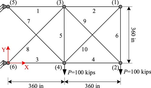
The configuration of the truss is presented in Figure 4. All members are made of aluminum in which the modulus of elasticity is E = 10,000 ksi (68,950 MPa) and the density is ρ = 0.1 lb/in³ (2768 kg/m³). The cross-sectional areas of truss members range from 0.1 to 35 in² (0.6–228.5 cm²). Constraints include both stresses and displacements. The stresses of all members must be lower than ±25 ksi (172.25 Mpa), and the displacements of all nodes are limited to 2 in (50.8 mm). This problem has been well investigated in the literature (Camp & Farshchin, 2014; Pham, 2016).

Figure 4. 10-bar truss.

5.1.2. 25-bar truss structure

The layout of the truss is presented in Figure 5. The mechanical properties are the same as in the 10-bar truss. The allowable horizontal displacement in this problem is ±0.35 in (8.89 mm). Members are grouped into eight groups with the allowable stresses as shown in Table 1. Hence, the number of design variables in this problem D = 8. The cross-sectional areas of the members vary between 0.01 and 3.5 in². Two loading cases acting on the structure are given in Table 2. Like the 10-bar truss structure, the 25-bar truss structure has been studied by many researchers (Camp & Farshchin, 2014; Pham, 2016).

Figure 5. 25-bar truss.

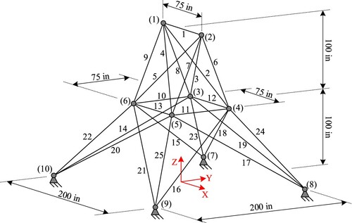
Table 1. Allowable stresses for 25-bar truss.

Group	Member	Allowable stress for compression (ksi)	Allowable stress for tension (ksi)
1	1	35.092	40.0
2	2, 3, 4, 5	11.590	40.0
3	6, 7, 8, 9	17.305	40.0
4	10, 11	35.092	40.0
5	12, 13	35.092	40.0
6	14, 15, 16, 17	6.759	40.0
7	18, 19, 20, 21	6.959	40.0
8	22, 23, 24, 25	11.082	40.0

Table 2. Load cases for 25-bar truss.

Node	Case 1			Case 2
	PX	PY	PZ	PX	PY	PZ
1	–	20.0	−5.0	1.0	10.0	−5.0
2	–	−20.0	−5.0	–	10.0	−5.0
3	–	–	–	0.5	–	–
6	–	–	–	0.5	–	–

5.1.3. 72-bar truss structure

This truss is displayed in Figure 6. The modulus of elasticity and the material density of this structure are similar to the two above structures. The displacements of all free nodes along both x and y directions are limited within ±0.25 in (6.35 mm) and the stresses of members must be smaller than ±25 ksi. Members are categorized into sixteen groups as shown in Table 3, and the cross-sectional area of each group is in the range [0.1, 4.0] in². This structure subjects to two independent load cases as listed in Table 4. This example has been carried out in some previous studies (Camp & Farshchin, 2014; Pham, 2016).

Figure 6. 72-bar truss.

Table 3. Member group for the 72-bar truss.

Group	Member	Group	Member	Group	Member	Group	Member
1	1–4	5	19–22	9	37–40	13	55–58
2	5–12	6	23–30	10	41–48	14	59–66
3	13–16	7	31–34	11	49–52	15	67–70
4	17, 18	8	35, 36	12	53, 54	16	71, 72

Table 4. Load cases for the 72-bar truss.

Node	Load Case 1 (kips)			Load Case 2 (kips)
	PX	PY	PZ	PX	PY	PZ
17	5.0	5.0	−5.0	–	–	−5.0
18	–	–	–	–	–	−5.0
19	–	–	–	–	–	−5.0
20	–	–	–	–	–	−5.0

5.2. Setup

Three above problems are optimized using both CoDE and SA-CoDE with the same parameters as follows: NP = 20, F_pool = [0.6, 0.8, 1.0], and Cr_pool = [0.1, 0.2, 1.0]. Three mutation strategies used in this study are ‘rand/1/bin’, ‘rand/2/bin’, and ‘current-to-rand/1’. A large penalty term is added to the objective function when any constraint is violated ensuring all infeasible vectors are omitted during the optimization process. The ϵ value for the ϵ-level comparison is fixed to 0.2. The optimization is finished after maxiter = 500 generations.

Particularly for the SA-CoDE, the number of generations of the first phase is iter1 = 50 while the number of generations of the second phase is iter2 = maxiter-iter1 = 450. It means the dataset collected after the first phase contains [3 × (iter1−1)+1] × NP = 2960 samples. However, for some samples, the truss structures are close to being unstable, leading to the large values of the constraint violation. These samples are considered outliers and should be cleaned up from the training data. Therefore, all samples having a constraint violation greater than 0.5 are deleted from the dataset.

Neural networks developed in all problems have the same architecture of (D-10D-10D-10D-1). The input layer consists of D neurons where D is the number of design variables (D = 10 for the 10-bar truss problem, D = 8 for the 25-bar truss problem, and D = 16 for the 72-bar truss problem). Three networks have also three hidden layers with 10D neurons per layer. There exists only one neuron in the output layer. Inputs of the surrogate models are the cross-sectional areas of truss members while the output is the constraint violation of such structure. The activation function used in this study is ReLU and the loss function is MSE. Neural networks are trained for 1000 epochs with a batch size of 10. The Adam algorithm is utilized to minimizing the loss function of neural networks. Before training, the input data should be normalized by dividing to the upper bounds of members’ cross-sectional areas.

In addition, the standard DE algorithm is also implemented with the mutation strategy ‘current-to-best/2/bin’. This variant is known as one of the powerful mutation strategies of the DE algorithm. The standard DE algorithm is implemented two times with the population size NP is set to be 20 (called the DE(20)) and 30 (called the DE(30)). Other parameters are as follows: the scaling factor F = 0.8, the crossover rate Cr = 0.9, maxiter = 500.

The experiments are carried out using the programming language Python. The finite element code for structural analysis is also written in Python based on the direct stiffness method. Neural network-surrogate models are developed using the ‘MLPRegressor’ feature from the open-source machine learning library Scikit-learn (Pedregosa et al., 2011). For all cases, 25 independents runs are performed. The computation is performed on a personal computer with the following configuration: CPU Intel Core i5-5257 2.7 GHz, RAM 8.00 Gb.

5.3. Results

Figures 7–9 plot the convergence histories for the 10-bar truss, the 25-bar truss, and the 72-bar truss, respectively.

Figure 7. Convergence histories of the CoDE and the SA-CoDE for the 10-bar truss.

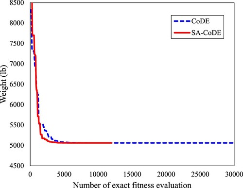
Figure 8. Convergence histories of the CoDE and the SA-CoDE for the 25-bar truss.

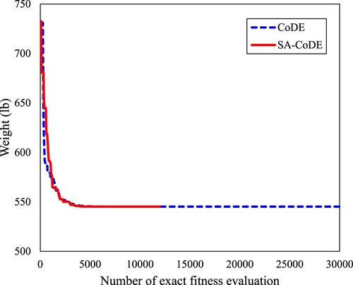
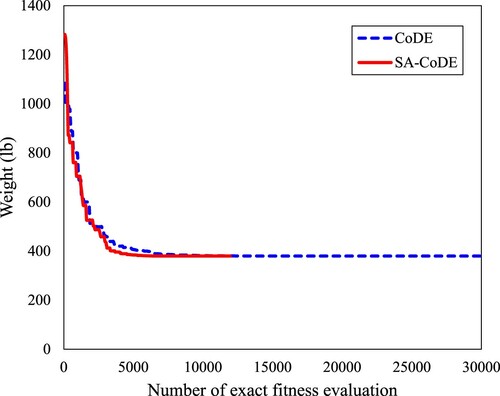
Figure 9. Convergence historyies of the CoDE and the SA-CoDE for the 72-bar truss.

The results obtained from the CoDE, the SA-CoDE, and the DE for 25 runs are reported in terms of best, mean, worst, and standard deviation (SD) values in Tables 5–7. The optimal designs found by the Differential Evolution with opposition-based mutation and nearest neighbor comparison (ODE-NNC) (Pham, 2016), and the modified Teaching-Learning Based Optimization (TLBO) (Camp & Farshchin, 2014) are also included for the comparison. Moreover, the required numbers of exact fitness evaluations are given in Table 8.

Table 5. Results for the 10-bar truss.

Member	TLBO (Camp & Farshchin, 2014)	ODE-NNC (Pham, 2016)	DE(20)	DE(30)	CoDE	SA-CoDE
1 (in^2)	30.668	30.534	30.585	30.522	30.522	30.522
2 (in^2)	0.100	0.100	0.100	0.100	0.100	0.100
3 (in^2)	23.158	23.211	23.107	23.202	23.200	23.197
4 (in^2)	15.223	15.228	15.164	15.225	15.223	15.226
5 (in^2)	0.100	0.100	0.100	0.100	0.100	0.100
6 (in^2)	0.542	0.552	0.560	0.551	0.551	0.551
7 (in^2)	7.465	7.457	7.470	7.457	7.457	7.457
8 (in^2)	21.026	21.036	21.062	21.036	21.036	21.037
9 (in^2)	21.466	21.507	21.548	21.526	21.528	21.528
10 (in^2)	0.100	0.100	0.100	0.100	0.100	0.100
Best (lb)	5060.973	5060.857	5060.890	5060.854	5060.854	5060.854
Worst (lb)	–	–	5079.637	5076.672	5076.669	5076.669
Mean (lb)	5064.808	5060.892	5065.144	5063.414	5061.385	5061.964
SD	6.371	0.035	5.907	5.590	2.838	4.002
Constraint violation	None	None	None	None	None	None

Table 6. Results for the 25-bar truss.

Group	TLBO (Camp & Farshchin, 2014)	ODE-NNC (Pham, 2016)	DE(20)	DE(30)	CoDE	SA-CoDE
1 (in^2)	0.0100	0.010	0.010	0.010	0.010	0.010
2 (in^2)	1.9878	1.987	1.987	1.987	1.987	1.987
3 (in^2)	2.9914	2.994	2.993	2.993	2.993	2.993
4 (in^2)	0.0102	0.010	0.010	0.010	0.010	0.010
5 (in^2)	0.0100	0.010	0.010	0.010	0.010	0.010
6 (in^2)	0.6828	0.684	0.684	0.684	0.684	0.684
7 (in^2)	1.6775	1.677	1.677	1.677	1.677	1.677
8 (in^2)	2.6640	2.663	2.662	2.662	2.662	2.662
Best (lb)	545.175	545.163	545.163	545.163	545.163	545.163
Worst (lb)	–	545.165	546.807	545.271	545.163	545.163
Mean (lb)	545.483	–	545.274	545.167	545.163	545.163
SD	0.306	0.003	0.349	0.022	0.000	0.000
Constraint violation	None	None	None	None	None	None

Table 7. Results for the 72-bar truss.

Group	TLBO (Camp & Farshchin, 2014)	ODE-NNC (Pham, 2016)	DE(20)	DE(30)	CoDE	SA-CoDE
1 (in^2)	1.881	1.885	1.892	1.893	1.887	1.877
2 (in^2)	0.514	0.514	0.511	0.513	0.511	0.518
3 (in^2)	0.100	0.100	0.100	0.100	0.100	0.100
4 (in^2)	0.100	0.100	0.100	0.100	0.100	0.100
5 (in^2)	1.271	1.267	1.281	1.262	1.271	1.270
6 (in^2)	0.515	0.514	0.516	0.512	0.513	0.514
7 (in^2)	0.100	0.100	0.100	0.100	0.100	0.100
8 (in^2)	0.100	0.100	0.100	0.100	0.100	0.100
9 (in^2)	0.532	0.525	0.527	0.525	0.523	0.516
10 (in^2)	0.513	0.515	0.509	0.515	0.517	0.516
11 (in^2)	0.100	0.100	0.100	0.100	0.100	0.100
12 (in^2)	0.100	0.100	0.100	0.100	0.100	0.100
13 (in^2)	0.157	0.157	0.156	0.156	0.156	0.157
14 (in^2)	0.543	0.545	0.547	0.545	0.545	0.545
15 (in^2)	0.408	0.410	0.408	0.411	0.412	0.407
16 (in^2)	0.573	0.569	0.573	0.570	0.568	0.569
Best (lb)	379.632	379.618	379.639	379.617	379.617	379.623
Worst (lb)	–	–	380.430	379.907	379.662	382.306
Mean (lb)	379.759	379.642	379.888	379.667	379.631	379.860
SD	0.149	0.024	0.216	0.057	0.013	0.545
Constraint violation	None	None	None	None	None	None

Table 8. Required number of exact fitness evaluations.

Approach	10-bar truss	25-bar truss	72-bar truss
TLBO	13,767	12,199	21,542
ODE-NNC	7000	5000	10,000
DE(20)	10,000	10,000	10,000
DE(30)	15,000	15,000	15,000
CoDE	29,960	29,960	29,960
SA-CoDE	11,960	11,960	11,960

Based on the obtained results, it can be pointed out some observations as follows. In general, the CoDE attains the best results among these algorithms. In detail, the best weights of the 10-bar truss, the 25-bar truss, and the 72-bar truss found by the CoDE are 5060.854, 545.163, and 379.617 lb, respectively. These values are slightly lower than the best weights found by the ODE-NNC and the TLBO. In addition, the best results found by the DE(30) are the same as the CoDE but the standard deviations of the DE(30) are larger than the corresponding values of the CoDE. It indicates that the CoDE is more stable than the DE(30). For the same population size of 20, the results obtained by the DE(20) are worse than those of the CoDE. The reason is that the CoDE employs three mutation strategies at the same time, leading to the strong ability to search over the design space.

Nonetheless, the convergence speed of the CoDE is very slow. With the same control parameters, the CoDE performs 29,960 exact fitness evaluations while the numbers for DE(20) and DE(30) are 10,000 times and 15,000 times, respectively. In other words, the CoDE is approximately 3 times slower than the DE(20) and 2 times slower than the DE(30).

Moreover, the SA-CoDE has also shown good results. The optimal weights of the 10-bar truss and the 25-bar truss found by the SA-CoDE are 5060.854 and 545.163 lb, respectively. These values are the same as the results of the CoDE and the DE(30). For the 72-bar truss, the best weight of the SA-CoDE equals 379.623 lb, which is slightly larger than the CoDE and the DE(30) (379.617 lb). But the advantage of SA-CoDE is its convergence speed. As shown in Table 8, the SA-CoDE performs only 11,960 evaluations while the required numbers of exact fitness evaluations of the DE(30) and the CoDE are 15,000 times and 29,960 times, respectively. It means the SA-CoDE is more than 2.5 times faster than the CoDE.

Comparing with previous studies, it is clearly seen that the SA-CoDE is better than the TLBO in terms of the best weight as well as the computation cost. The optimal weight of the SA-CoDE is better than the ODE-NNC for the 10-bar truss but worse than ODE-NNC for the 72-bar truss. However, the numbers of fitness evaluations carried out by the ODE-NNC are much smaller than those of the SA-CoDE for all three structures.

In summary, the experiment results show that the proposed approach SA-CoDE is a promising solution. Compared to the CoDE, the SA-CoDE accomplishes the same results but it saves the computation cost by reducing the number of exact fitness evaluations.

5.4. Influence of the number of training samples

In this section, the 10-bar truss is optimized using the SA-CoDE for four times, in which the number of generations of the first stage iter1 is set to 10, 25, 50, and 100, respectively. Other parameters are the same for all cases. The statistical results of four cases are given in Table 9. It can be found that the computation cost of the first case (iter1 = 10) is the smallest but the optimal weight is larger than those of the remaining cases. When the number of generations of the first stage reaches 25, the best weight achieves 5060.854 lb. The result does not improve despite increasing the number of training samples. Overall, the recommended value of the parameter iter1 is in the range [25,50].

Table 9. Influence of the training data size.

Number of generations of the first stage iter1	10	25	50	100
Number of training samples	560	1460	2960	5960
Best (lb)	5060.855	5060.854	5060.854	5060.854
Mean (lb)	5063.275	5061.921	5061.964	5062.327
Worst (lb)	5076.670	5076.669	5076.669	5076.669
SD (lb)	4.999	3.942	4.002	4.419
Number of exact fitness evaluations	10,360	10,960	11,960	13,960

6. Conclusions

The study proposed an approach, called SA-CoDE, to enhance the CoDE algorithm in structural optimization. By using neural network-based surrogate models, the convergence speed is increased while still maintaining the powerful search capacity. This is a meaningful result, especially for computationally expensive optimization problems like structural optimization. The performance of the SA-CoDE is investigated through three well-known truss optimization problems. In all problems, the SA-CoDE provides similar results but it uses fewer exact fitness evaluations than the CoDE. Quantitatively, the SA-CoDE reduces the number of exact fitness evaluations by about 60% compared to the CoDE.

This work carries out surrogate models built using neural networks. In the future, methods to improve the accuracy of the surrogate model will be studied, and other structural optimization problems will be investigated.

Acknowledgments

The first author was funded by Vingroup Joint Stock Company and supported by the Domestic Ph.D. Scholarship Programme of Vingroup Innovation Foundation (VINIF), Vingroup Big Data Institute (VINBIGDATA) code VINIF.2020.TS.134.

Disclosure statement

No potential conflict of interest was reported by the author(s).

Additional information

Funding

This research is funded by the Domestic Ph.D. Scholarship Programme of Vingroup Innovation Foundation (VINIF), code VINIF.2020.TS.134.

Notes on contributors

Tran-Hieu Nguyen

Tran-Hieu Nguyen is currently a lecturer at National University of Civil Engineering (NUCE), Hanoi, Vietnam and PhD student in NUCE. He received the MSc degree in 2012 at NUCE. His main research interests are structural optimization, artificial intelligence and steel structures. Email: [email protected].

Anh-Tuan Vu

Anh-Tuan Vu received his PhD in 2009 at Bauhaus University Weimar, Germany. He is currently the head of the Department of Steel and Timber Constructions, NUCE. His main research interests are structural optimization, steel structures, steel and concrete composite structures. Email: [email protected].

References

- Bureerat, S., & Pholdee, N. (2016). Optimal truss sizing using an adaptive differential evolution algorithm. Journal of Computing in Civil Engineering, 30(2), 04015019. https://doi.org/https://doi.org/10.1061/(ASCE)CP.1943-5487.0000487
- Cai, J., & Thierauf, G. (1996). Evolution strategies for solving discrete optimization problems. Advances in Engineering Software, 25(2-3), 177–183. https://doi.org/https://doi.org/10.1016/0965-9978(95)00104-2
- Camp, C. V., & Farshchin, M. (2014). Design of space trusses using modified teaching–learning based optimization. Engineering Structures, 62-63, 87–97. https://doi.org/https://doi.org/10.1016/j.engstruct.2014.01.020
- Deb, K. (2000). An efficient constraint handling method for genetic algorithms. Computer Methods in Applied Mechanics and Engineering, 186(2-4), 311–338. https://doi.org/https://doi.org/10.1016/S0045-7825(99)00389-8
- Ho-Huu, V., Nguyen-Thoi, T., Vo-Duy, T., & Nguyen-Trang, T. (2016). An adaptive elitist differential evolution for optimization of truss structures with discrete design variables. Computers & Structures, 165, 59–75. https://doi.org/https://doi.org/10.1016/j.compstruc.2015.11.014
- Jia, G., Wang, Y., Cai, Z., & Jin, Y. (2013). An improved (μ+ λ)-constrained differential evolution for constrained optimization. Information Sciences, 222, 302–322. https://doi.org/https://doi.org/10.1016/j.ins.2012.01.017
- Kim, S. E., Vu, Q. V., Papazafeiropoulos, G., Kong, Z., & Truong, V. H. (2020). Comparison of machine learning algorithms for regression and classification of ultimate load-carrying capacity of steel frames. Steel and Composite Structures, 37(2), 193–209. https://doi.org/https://doi.org/10.12989/scs.2020.37.2.193
- Krempser, E., Bernardino, H. S., Barbosa, H. J., & Lemonge, A. C. (2012). Differential evolution assisted by surrogate models for structural optimization problems. In Proceedings of the international conference on computational structures technology (CST). Civil-Comp Press (Vol. 49).
- Mallipeddi, R., & Lee, M. (2012, June). Surrogate model assisted ensemble differential evolution algorithm. In 2012 IEEE congress on evolutionary computation (pp. 1–8). IEEE.
- Mallipeddi, R., Suganthan, P. N., Pan, Q. K., & Tasgetiren, M. F. (2011). Differential evolution algorithm with ensemble of parameters and mutation strategies. Applied Soft Computing, 11(2), 1679–1696. https://doi.org/https://doi.org/10.1016/j.asoc.2010.04.024
- Nguyen, T. H., & Vu, A. T. (2020). Using neural networks as surrogate models in differential evolution optimization of truss structures. In International conference on computational collective intelligence (pp. 152–163). Springer, Cham.
- Nguyen, T. H., & Vu, A. T. (2021). A comparative study of machine learning algorithms in predicting the behavior of truss structures. In Kumar R, Quang N.H, Solanki V.J, Cardona M, & Pattnaik P.K (Eds.), Research in intelligent and computing in engineering (pp. 279–289). Springer, Singapore.
- Pedregosa, F., Varoquaux, G., Gramfort, A., Michel, V., Thirion, B., Grisel, O., Blondel, M., Prettenhofer, P., Weiss, R., Dubourg, V., Vanderplas, J., Passos, A., Cournapeau, D., Brucher, M., Perrot, M., & Duchesnay, E. (2011). Scikit-learn: Machine learning in Python. Journal of Machine Learning Research, 12(Oct), 2825–2830.
- Pham, H. A. (2016). Truss sizing optimization using enhanced differential evolution with opposition-based mutation and nearest neighbor comparison. Journal of Science and Technology in Civil Engineering (STCE)-NUCE, 10(5), 3–10.
- Rahnamayan, S., Tizhoosh, H. R., & Salama, M. M. (2008). Opposition-based differential evolution. IEEE Transactions on Evolutionary Computation, 12(1), 64–79. https://doi.org/https://doi.org/10.1109/TEVC.2007.894200
- Rajeev, S., & Krishnamoorthy, C. S. (1992). Discrete optimization of structures using genetic algorithms. Journal of Structural Engineering, 118(5), 1233–1250. https://doi.org/https://doi.org/10.1061/(ASCE)0733-9445(1992)118:5(1233)
- Rosenblatt, F. (1958). The perceptron: A probabilistic model for information storage and organization in the brain. Psychological Review, 65(6), 386–408. https://doi.org/https://doi.org/10.1037/h0042519
- Rumelhart, D. E., Hinton, G. E., & Williams, R. J. (1986). Learning representations by back-propagating errors. Nature, 323(6088), 533–536. https://doi.org/https://doi.org/10.1038/323533a0
- Storn, R., & Price, K. (1997). Differential evolution–a simple and efficient heuristic for global optimization over continuous spaces. Journal of Global Optimization, 11(4), 341–359. https://doi.org/https://doi.org/10.1023/A:1008202821328
- Takahama, T., Sakai, S., & Iwane, N. (2006, October). Solving nonlinear constrained optimization problems by the ϵ constrained differential evolution. In 2006 IEEE International conference on systems, man and cybernetics (Vol. 3, pp. 2322–2327). IEEE.
- Truong, V. H., Vu, Q. V., Thai, H. T., & Ha, M. H. (2020). A robust method for safety evaluation of steel trusses using Gradient Tree Boosting algorithm. Advances in Engineering Software, 147, 102825. https://doi.org/https://doi.org/10.1016/j.advengsoft.2020.102825
- Wang, Y., & Cai, Z. (2011). Constrained evolutionary optimization by means of (μ+ λ)-differential evolution and improved adaptive trade-off model. Evolutionary Computation, 19(2), 249–285. https://doi.org/https://doi.org/10.1162/EVCO_a_00024
- Wang, Y., Cai, Z., & Zhang, Q. (2011). Differential evolution with composite trial vector generation strategies and control parameters. IEEE Transactions on Evolutionary Computation, 15(1), 55–66. https://doi.org/https://doi.org/10.1109/TEVC.2010.2087271
- Wang, B. C., Li, H. X., Li, J. P., & Wang, Y. (2019). Composite differential evolution for constrained evolutionary optimization. IEEE Transactions on Systems, Man, and Cybernetics: Systems, 49(7), 1482–1495. https://doi.org/https://doi.org/10.1109/TSMC.2018.2807785
- Wang, Z., Tang, H., & Li, P. (2009, December). Optimum design of truss structures based on differential evolution strategy. In 2009 international conference on information engineering and computer science (pp. 1–5). IEEE.
- Zhang, J., & Sanderson, A. C. (2009). JADE: Adaptive differential evolution with optional external archive. IEEE Transactions on Evolutionary Computation, 13(5), 945–958. https://doi.org/https://doi.org/10.1109/TEVC.2009.2014613