The application of machine learning and deep learning in sport: predicting NBA players’ performance and popularity

ABSTRACT

Basketball is known for the vast amount of data collected for each player, team, game, and season. As a result, basketball is an ideal domain to work on different data analysis techniques to gain useful insights. In this study, we continued our previous study published in 2020 Computational Collective Intelligence (12th International Conference, ICCCI 2020, Da Nang, Vietnam, November 30 – December 3, 2020, Proceedings) reviewing some important factors to predict players’ future performance and being selected in an All-Star game, one of the most prestigious events, of National Basket Association league. Besides traditional Machine Learning, Deep Learning is also applied in this study for prediction purpose. However, compared to traditional Machine Learning, Deep Learning’s performance is not as good for our dataset. It is understandable when our data are relatively small and structured with a few predictor variables which limited Deep Learning’s ability to deal with a vast amount of Big Data. Our final results, through both Regression and Classification Analysis, indicated that scoring is the most important factor from the primary players for any team and also basketball fan’s favourable style.

KEYWORDS:

• Data mining
• machine learning
• deep learning
• sport
• imbalanced data

1. Introduction

National Basketball Association (NBA) league is one of the most popular sport events in America and the most well-known basketball league over the world. NBA’s business is worth billions of dollars in the last few decades with millions of viewers and commercials. In the 2018–2019 season, the combined avenue of teams of the NBA was at a record of over 8.7 billion dollars, according to Statista. Forbes magazine showed the top five NBA teams have a worth network of $16.8 billion. Game broadcasts and advertisements during the streams are the generating most profit for NBA (Forbes 2019).

The purpose of our study is to evaluate the effectiveness of applying Machine Learning (ML) and Deep Learning (DL) on Sport Domain, particularly basketball, in perspective of manpower (players). Most prior studies paid more attention to predicting the outcomes of games or using ML or DL along with advanced technical tools to collect and analyse sport players’ data. Our approach is to target the widely available dataset, tracking players’ primary statistics, which would be used without the need for any complex technical tools, and use advanced ML and DL to explore the useful information and have an evaluation about the performance of various ML and DL models in basketball dataset. Based on this, our two primary objectives were to predict players’ future performance and popularity through modelling on players’ statistics collected in their regular games.

Regarding our second goal of forecasting players’ popularity, we concentrated on the forecast if players are chosen to play in the next season NBA All-Star game. NBA All-star game is an annual February exhibition event in which 24 NBA star players are divided into 2 teams to compete. The procedure to choose players participating in NBA All-star games involves a voting poll from fans, which has a vigorous influence on selection outcome. Thus, ‘Being selected in NBA All-star roster’ is a good indicator for us to evaluate players’ public popularity. In contrast to the effect of player’s performance on the court, the benefit of player’s popularity is not clear to recognize, so we would like to summarize briefly two essential aspects in perspective of business value creation from popular players.

First of all, popular or star players can have a significant contribution to their franchises’ brands among the teams in the league (Pifer et al., 2015). Athletes with strong on-field performance have a better ability to establish their star player’s attributes into a realized equity for a team’s brand, thus raising the awareness for a team, getting the public attention and assisting in reaching the new market. Secondly, through different economic models, star players generate externalities that increase attendance and other revenue sources beyond their individual contributions to team success (Humphreys & Johnson, 2020; Berri & Schmidt, 2006). In other words, they not only lead their own teams to win games but also attract more fans and gain public attention to increase overall league’s business revenue and media coverage, even for their opponents. The historical data showed the superstar effect on the economy throughout different eras.

With the rapid development of data science in recent years, Machine learning (ML) and Data mining (DM) have been applied in various fields. As a result of this movement, Sport Analytics, a field where ML methods and its implementations are used to gain useful insights from sport data (Apostolou & Tjortjis, 2016), has been emerging as one of the favourable areas for both business and academic research. As Sport Analytics has become more prominent and attainable, sport teams, coaches, players and companies are more likely to use its applications to improve their performance and operation on- and off-the court (Tichy, 2016). In terms of sport domain, there have been many academic studies and systematic frameworks developed for basketball using ML and DM techniques with the purposes of long-term strategy, daily operation and prediction in professional leagues or college/high school (Thabtah et al., 2019; Miljković et al., 2010; Zuccolotto et al., 2018).

It is our effort to study further various advanced technological methodologies from our previous paper in 2020 Computational Collective Intelligence (12th International Conference, ICCCI 2020, Da Nang, Vietnam, November 30 – December 3, 2020, Proceedings) which we applied data mining by ML models on identical basketball datasets and achieved good results with RMSE of 2.1969 and MAE of 1.6465 for the first objective and Recall of 0.9657 and ROC AUC of 0.9096 for the second objective, respectively (Nguyen, et al., 2020). Based on our previous study, we decided to extend further in providing information about our understanding of each ML model and its mechanism, so it can provide a reason why it was chosen in our study. Moreover, we paid extra times on data collection and preparation for each variable (feature) to assure the accuracy and understand more relationships among basketball players’ attributes.

In addition, besides traditional ML applied in our previous study, the potential of deep learning was also covered. Deep learning has been recently one of the most popular techniques used in computer vision, natural language processing or sentiment analysis. Deep learning is a statistical technique using neural networks with multiple layers, essentially for pattern classification (Marcus, 2018). Although Deep learning has the limitation as it works like a ‘black box’ and we cannot really observe how each predictor variable affects the final prediction, it is still drawing the attention from both the scientific and business community by its extraordinary competence in prediction. Our study aims is to examine how effective Deep learning deals with structured and relatively small datasets to make the prediction and compare its performance to the traditional Machine Learning for our basketball dataset.

CRISP-DM methodology is used as the reference to construct ML and DL models. The greatest benefit is to provide a common method for communication that helps to connect a variety of technical tools and people with different skills and backgrounds to progress an efficient and effective project (Wirth & Hipp, 2000). As a typical CRISP-DM, our study was divided into six phases:

1. Business understanding: understanding the issue from a business perspective to define data mining goal. Our understanding was conducted thoughtfully through reviewing a considerable number of published articles;

2. Data understanding: collecting the data, learning data characteristics, data quality issues;

3. Data preparation: data cleaning and manipulation for modelling;

4. Modelling: several modelling algorithms are trained to choose the most qualified one;

5. Evaluation: based on the predetermined objectives, criteria and metrics, models are appraised;

6. Deployment: direction to deploy the ML model into production.

The study concentrated on the first five phases, while the final phase provided the limitation for future improvement.

2. Literature review

There have been several published research studies applying machine learning and deep learning to predict results in a variety of sports. The application of data mining in basketball was started in the 1990s by IBM named Advanced Scout (Colet & Parker, 1997). The purpose of this tool was to assist the NBA management team to discover the hidden patterns from basketball statistics using data mining techniques. The system used a data mining technique called Attribute Focusing. This technique compared the overall distribution of an attribute to its distributions from different subsets of data. Then, if any subset shows a characteristically different distribution, the combination of attributes describing the subset is marked as ‘interesting’. However, the technique mostly raised the awareness (similarly as anomaly detection nowadays) about some unusual data distribution with a limited explanation or interpretation about players’ statistics.

Hidden Markov Models (HMMs) were used in recent times to model the progression of match results (wins/losses) through different times by applying advanced statistics from NBA games as features and be able to predict the match result achieving a prediction accuracy of 73% (Madhavan, 2016). Rue and Slavensen used a Bayesian approach, combined with Markovian chains and the Monte-Carlo method, to predict football game results (Rotshtein et al., 2015). However, as it used the Neural network for predictive ability enhancement, the approach lacked interpretability and hence cannot be used for performance analysis or feedback. In another paper, a Bayesian hierarchical model was also applied to predict football results based on scoring intensity data determined by the attack and defence strength of the two teams involved (Maher, 1982).

Leung and Joseph (2014) proposed a data mining technique to predict the outcomes of sport games and discover useful insights. By testing in practical data from college football games, the proposed technique showed positive results with high accuracy in prediction. Their technique is based on a combination of four different measures on the historical results of the games. The core concept is to predict the outcome of the game between two teams through analysing a set of teams that are most similar to each of the competing teams, finding the results of the games between the teams in each of the two sets, and using those game results for prediction.

Zifan Shi, Sruthi Moorthy, and Albrecht Zimmermann used Machine Learning techniques specialized in classifier learning for the purpose of predicting the outcome of NCAAB matches (Zimmermann et al., 2013). The research discovered some interesting facts that were unexpected in the scientific community. In the context of 2013, an ML technique – multi-layer perceptron which was not widely used, was proved to be the most effective in the explored settings. Moreover, explicit modelling the differences between NCAAB teams’ attributes did not improve the model predictive accuracy. Finally, the most impressive fact was that there seemed to be a great milestone of 74% predictive accuracy that could not be exceeded by ML or statistical techniques.

Deep learning (Artificial Neural Network) has also become more popular in sport prediction. The prediction model of National Football League (NFL) team winning by Kahn was able to reach the accuracy of 75%, nearly 10% higher than the prediction by domain experts in NFL. The model was treated as a classification model which was an improvement from the previous model which was done by Purucker’s study (Kahn, 2003). In Kahn’s model, data were collected from 208 games in the 2003 season. The Neural Network (NN) 10-3-2 (10 nodes in input layers, 3 nodes in hidden layers, and 2 nodes in the output layers) was used to achieve the result.

Similarly, a 20-10-1 NN model, designed by McCabe and Trevathan, was able to predict results in four different sports (Rugby League, Australian Rules football, Rugby Union, and English Premier League Football) using previous season data that had also achieved an average accuracy result of 67.5% (McCabe, & Trevathan, 2008). Same variables across different sports were used to build the model.

Through many studies for both Traditional ML and DL, the focus was mostly on predicting the outcomes of the games, while there is no actual research for individual players’ performance and popularity, which was mentioned in the Introduction to have a significant influence on team’s outcome and revenue. Thus, our study paid more attention to this aspect to provide analytical models to evaluate and forecast individual players by ML and DL with high accuracy. Moreover, the comparison among the models’ results could give a brief overview about the performance between Traditional ML and DL in relatively small (basketball) dataset for prediction purpose.

3. Materials

3.1. Data sources

The first dataset is NBA players’ stats since 1950 from the website basketball-reference.com. Since there are many unavailable and inconsistent data for variables, only data from 1979 were implemented including players’ information and their basketball stats, which can be divided into 2 categories: ‘cumulative’ variables – number of games played (G), total minutes played (MP), total points (PTS), … and its ‘percentage’ variables – percentage of 2 points made on total attempts in a given season (%2P), percentage of 3 points (%3P), … The dataset also includes our target variable for the first objective – WS.

The second dataset is from the website basketball.realgm.com archiving all NBA All-star rosters in each year and it was merged with the first dataset in the Data Preparation step based on two mutual variables: year and players’ names, to find out if a player was chosen to play in All-Star games coded as binary target variable: 1 if selected for NBA All-star roster and 0 if not.

3.2. Data summary

Observing the target variable for the second objective, there is an issue with imbalanced data as the percentage of All-Star players is only 6. Technically, imbalanced data exhibit an unequal distribution between its classes, or one class severely out-represents another, particularly between-classes in this case (He & Garcia, 2009). Two potential solutions were proposed: under-sampling and over-sampling techniques. Moreover, as our priority is to detect potential ‘All-Star’ players, two metrics: ROC AUC and Recall scores are our primary options. Overall, some popular evaluation metrics in ML field were selected to assess and compare our ML algorithms:

1. Root Mean Squared Error (RMSE) and Mean Absolute Error (MAE) for the regression models

2. Accuracy, Precision, especially Recall and Receiver operating characteristic area under curve (ROC AUC) and F1 scores for the classification models.

3.3. Data preparation

The reason for missing values in ‘percentage’ variables is that there was no attempt or success from players, so we assumed that no attempt was similar to no success and missing values for these variables were imputed by zero-value.

There are 19 predictor variables used in our first objective’s regression model: G, MP, PTS, FG%, 2P%, 3P, 3P%, FT%, AST, AST%, BLK, BLK%, DRB, DRB%, ORB, STL, STL%, TOV% and PF. For the purpose of our first objective, the original dataset was firstly partitioned into training-test sets with the ratio of 80–20. Then, our training set was divided again into train-valid sets with the ratio of 80–20. The train set was used to train the model with the cross-validation technique. Then, train-valid sets were used to evaluate models under the potential over-fitting condition. Test set would be used for our Evaluation phase to estimate how effective our final model is when it is used for unseen data. To eliminate the case when players’ data in some periods of time were sampled into train/valid/test sets unevenly, stratified sampling technique was adopted, using Year ratio.

The primary difference for data engineering between the first and second objectives and between our first paper and this one is that we considered the factor (predictor variable) being selected for this season All-Star game to predict players’ probability being the next season All-Star players. The train-valid-test splitting process was also used for our second objective. As mentioned in the Data Summary section, one issue with the original data is class imbalance which can affect the model evaluation and performance, so two popular solutions: over-sampling and under-sampling, were applied for this study, which aimed to ease the effect of imbalanced data distribution on learning process (Batista et al., 2004; Chawla et al., 2002; Chawla et al., 2004). Besides random over-sampling, synthetic minority oversampling technique (SMOTE) was also used for over-sampling purpose, which is widely adopted in many applications for different domains, such as network intrusion detection (Cieslak et al., 2006), breast cancer detection (Fallahi & Jafari, 2011), or biotechnology (Batuwita & Palade, 2009). Its methodology is to create new minority class examples through randomly choosing one (or more depending on the defined over-sampling ratio) of the k nearest neighbours (kNN) of a minority class instance and then generation of the new instance values from a random interpolation of both instances (Galar et al., 2011), so it would help to reduce the potential effect of over-fitting from random over-sampling. Another popular sampling technique used for our study is under-sampling, which targets to balance class distribution through the random elimination of majority class instances and is proved in many studies to outperform SMOTE or random over-sampling in most situations for both low- and high-dimensional data (Hulse et al., 2007; Blagus & Lusa, 2013; Drummond & Robert, 2003).

4. Traditional machine learning method and results

4.1. Regression analysis

To select the best model for our first objective – WS, first six candidate models were trained with the train data using 10-fold cross-validation (CV). Then, all models were compared by its results on train and valid datasets, so we could find the most fitted model under different scenarios. RMSE and MAE are two metrics used for evaluation, as mentioned in Section 2.2.

Regression model types: Linear Regression (linear_model), Gradient Boosting Machine (gradient_boosting), Linear Support Vector Machine (linear_svm), Polynomial (Non-Linear) Support Vector Machine (poly_svm), Random Forest (random_forest), and Neural Net (neural_net) were used as the first candidate models.

4.1.1. Linear regression

Linear regression is the most fundamental form of modelling started in 1805 by Legendre and in 1809 by Gauss as the least squares method (Yan & Su, 2009). It requires that the model is linear in regression parameters with the purpose of discovering the relationship between one or more response variables and the predictors.

4.1.2. Gradient boosting machine

The idea of a gradient boosting machine is to modify multiple weak learners to become better (Michael Kearns articulated the goal as the ‘Hypothesis Boosting Problem’) (Yanofsky, 2015). A gradient boosting involves 3 elements: a loss function to be optimized, a weak learner to make prediction, and an additive model to add weak learners to minimize the loss function.

Decision trees are used as the weak learner in gradient boosting.

Trees are added one at a time, and existing trees in the model are not changed. A gradient descent procedure is used to minimize the loss when adding trees. After calculating the loss, to perform the gradient descent procedure, we must add a tree to the model that reduces the loss (such as following the gradient). We do this by parameterizing the tree, then modify the parameters of the tree and move in the right direction by reducing the residual loss (Brownlee, 2016).

4.1.3. Support vector machine

Support Vector Machine is a supervised learning model developed at AT&T Bell Laboratories by Vladimir Vapnik with colleagues (Boser et al., 1992; Bromley et al., 1993; Drucker et al., 1997) and is known as one of the most robust prediction methods. Although it is also widely used for regression, Support Vector Machine is more popular for its versatility in classification purposes. Thus, more details about Support Vector Machine are provided in our second objective of classification.

4.1.4. Random forest

Random forest is a robust machine learning algorithm as an ensemble method made up of a large number of small decision trees (estimators) with its own predictions. The algorithm can do classification prediction but slightly less good at regression because it is unable to make predictions outside the range of its training data. Similarly, to Support Vector Machine, more details about Random Forest are provided in our second objective of classification.

4.1.5. Neural network

Neural Networks or Artificial Neural Networks are a set of complex algorithms, modelled after a human brain. As we can have a specific section – Deep Learning, for only currently well-developed Neural Networks, the details about Neural Networks will be discussed further later. Neural Network, which is applied in this section, is just a simple and default-parameterized modelling compared to the models developed in the Deep Learning section.

4.1.6. Train-valid data results

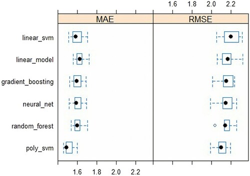
As shown in Figure 1, using 10-fold cross-validation on train set, 3 models with the best results for RMSE and MAE are as follows: gradient_boosting, neural_net and poly_svm with lower means or ranges of their result distributions. The MAE’s means of 3 best models range from 1.53 to 1.62 and they are around 2.12–2.15 for RMSE’s means, while the ranges of MAE are [1.47,1.70] and [2,2.27] for RMSE.

Figure 1. Distributions of cross-validation results for train data from six candidate regression models.

Then, our 7 candidate models were evaluated on valid data. As shown in Figure 2, gradient_boosting, neural_net and poly_svm are still the best three algorithms. However, neural_net and poly_svm results were worse in terms of RMSE metric compared to its medians from CV on train data. On the other hand, gradient_boosting keeps a steady outcome with only small increases, 0.02 for RMSE and 0.01 for MAE.

Figure 2. MAE and RMSE results for valid datasets from candidate regression models.

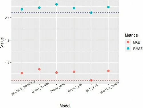
In conclusion, we decided to use Gradient Boosting Machine as our final model because of the following three reasons: (1) Gradient Boosting Machine has decent and stable results with both train and valid data with small changes of RMSE and MAE. (2) The differences between Gradient Boosting Machine and top performing models (usually Polynomial Support Vector Machines) at MAE and RMSE are small which is acceptable for our data mining’s first objective. (3) Gradient Boosting Machine is less subjective to over-fitting and performs much faster compared to Polynomial Support Vector Machines and Neural Net.

For model tuning, manual grid search was used with 135 combinations based on following four parameters: (1) Learning rate: [0.01, 0.1, 0.3]; (2) Depth of trees: [1, 2, 3, 4, 5]; (3) Minimum number of observations in the terminal nodes of the trees: [5, 10, 15]; (4) Subsampling: [0.65, 0.8, 1]. Model was tuned by all train and valid datasets with CV of 5 to find the optimal number of trees with maximum of 1000, and RMSE was used as a primary metric. With lowest RMSE of 2.1467, these parameters: (1) learning rate = 0.1, (2) depth of trees = 4, (3) minimum number of observations = 15, (4) subsampling = 0.8, and the optimal number of trees of 358; were used to train our final regression model.

4.1.7. Final result on test data

Final regression model was evaluated on test dataset (20% of the original data) and had 2.1969 for RMSE and 1.6465 for MAE. Compared to its RMSE on train-valid data, its RMSE result on test dataset is just over within 3% which can be considered satisfactory.

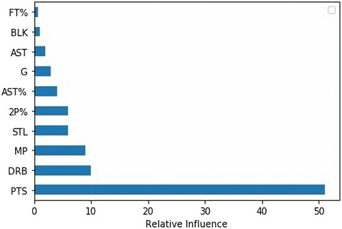
Observing Figure 3 – Top 10 relative features of our regression model, PTS is the most important feature with the relative influence of 51.56, while the second one – DRB – defensive rebound, has only 9.78. It was little surprised that there is not any 3-point variable in top 10 even it can be seen that 3-point play is really popular in NBA games nowadays when almost every team and player reply heavily on 3-point scoring. It can be explained that our analysis used many players’ statistics in the past seasons, while 3-point playing tactic has been only extremely popular for the past 10 years. Moreover, games are still dependent heavily on 2-point successful attempts as the ratio of total 2-point successful attempts on total 3-point successful attempts is 3.63 from season 2012–2013 to season 2016–2017.

Figure 3. Top 10 Relative features for final regression model by traditional machine learning.

4.2. Classification analysis

Firstly, popular ML classifiers: logistic regression (LG), Stochastic gradient descent (SGD), linear or polynomial support vector machine (LSVM or PSVM), random forest (RF) and Naïve Bayes (NB), were trained with both random and SMOTE over-sampling cases and were compared by Recall and ROC AUC scores. Two representative boosting algorithms, AdaBoost (AB) and Gradient Boosting Machine (GBM), were also employed for comparison. As the under-sampling technique has a drawback of potentially removing the useful information (Galar et al., 2011), the under-sampling methodology was applied for two bragging-related algorithms, balanced bragging classifier (BB) and balanced random forest classifier (BRF).

4.2.1. Logistic regression

Logistic regression model is another form of the linear regression model used for the case to predict variables as discrete class labels. For classification or, particularly, binary classification problems, the original linear function is extended by the logistic function with the output ranging from 0 to 1 and interpreted as the probability that the target variable is 1 given the input data.

Although logistic regression is also a popular classification model in the sport domain for its capability for complex classification models, it has a drawback of failing to capture non-linear relationships between features (Hosmer & Lemeshow, 2000).

4.2.2. Stochastic gradient descent

Stochastic gradient descent optimizes the objective function by relevant smoothness properties as an iterative progress. The algorithm replaces calculating the entire dataset (actual gradient) by calculating a randomly selected subset of the data (estimation), so it is considered as stochastic approximation of gradient descent optimization. Thus, for high-dimensional optimization problems, this method supports faster iterations and reduces the computational burden but achieves a lower convergence rate (Bottou & Bousquet, 2012)

4.2.3. Support vector machine

Support Vector Machine (SVM) algorithm optimizes the model by maximizing the geometric margin separating classes. As a result, there is a problem of constrained optimization as we try to achieve maximal margin hyper-plane and also ensure that all samples are separated by the margin. Boser et al., 1992 introduced the Karush-Kuhn-Tucker (KKT) condition to solve this issue (Burges, 1998). In addition, the kernel trick parameter can be used to transform non-linearly separable features into high-dimensional feature space such as polynomial kernel or Gaussian kernel.

4.2.4. Random forest

As mentioned in the first objective, random forest (RF) uses a large number of decision trees to reduce the variance of prediction, and converge the best possible prediction based on the majority. RF was introduced by Breiman (1996) besides other designs such as RF based on conditional inference trees (Hothorn et al., 2006). The prediction for new observations is based on the aggregation of multiple predictions made by single decision trees included in the RF algorithm through average results for regression RF or majority voting for classification RF.

4.2.5. Naive Bayes

The Naive Bayes Classifier is one of the simplest algorithms among classifiers. Its mechanism is based on the assumption that samples’ attributes are conditionally independent of samples’ class label meaning the probability of samples in a class is the multiplication of all conditional probabilities of attributes. Although it has a simple structure, it would still possibly outperform more sophisticated classification models (Langley et al., 1992).

4.2.6. Boosting algorithms

Boosting is constructed on the methodology of repeating a given weak learning algorithm on various distributions over the training data, and then combining the classifiers produced by the weak learner into a single composite classifier (Freund et al., 1997). This would benefit learning minority class through assigning weighted voting to outputs for each learner in the final prediction model to focus more on hard examples (Schwenk & Bengio, 1997; Guo & Herna, 2004).

4.2.7. Bragging algorithms

The core concept of Bragging modelling techniques is to use bootstrap aggregating (Breiman, 1996) to construct ensembles where a classification tree is induced by drawing a bootstrap sample from the minority class and the same number of randomized drawn cases, with replacement, from the majority class (Chen et al., 2004). Some research showed the effort of artificially balancing the classes provides some improvement effective with respect to a given performance measurement for tree classifier and under-sampling seems to have advantage over over-sampling (Drummond & Robert, 2003; Ling & Li, 1998; Kubat & Matwin, 1997). Besides, an under-sampling boosting algorithm (BU) was also involved in the comparison.

4.2.8. Train-valid data results

The results of applying 5-fold CV on random and SMOTE over-sampling train data are shown in Table 1. Among over-sampling algorithms, RF classifier had exceptional outcomes compared to others with nearly perfect recall scores for both random and SMOTE over-sampling data and ROC AUC scores at 0.990 and 0.964, respectively, followed by GBM classifiers with recall and ROC AUC scores at around 0.94–0.97. RF and GBM algorithms were then trained by two cases: random and SMOTE over-sampling, and made predictions on valid data, so we would compare their best results to under-sampling algorithms trained by original train data.

Table 1. Cross-validation results on random-, SMOTE over-sampling and under-sampling without predictor variable ‘being selected for this season all-star game’ for train data.

Models	Random over-sampling				SMOTE over-sampling
	Precision	Recall	ROC AUC	F1	Precision	Recall	ROC AUC	F1
LG	0.892	0.920	0.900	0.910	0.900	0.936	0.918	0.916
SGD	0.890	0.910	0.900	0.900	0.883	0.951	0.913	0.916
LSVM	0.880	0.930	0.904	0.910	0.890	0.948	0.916	0.918
PSVM	0.885	0.930	0.904	0.907	0.901	0.954	0.924	0.927
RF	0.980	1.000	0.9900	0.9900	0.959	0.981	0.964	0.970
NB	0.806	0.910	0.845	0.855	0.810	0.921	0.852	0.862
AB	0.905	0.918	0.911	0.911	0.910	0.932	0.920	0.921
GBM	0.918	0.970	0.9420	0.943	0.926	0.959	0.941	0.942

When applying predictor variable ‘Being selected for this season All-Star game’ for our candidate models, Table 2 shows similar results as Table 1. RF classifier and GBM models showed better results than other models, and they have slightly higher scores when using the Random Over-Sampling technique. Compared to results in Table 1, ‘Being selected for this season All-Star game’ variable helps RF classifier improve marginally for ROC AUC for 0.0001, while it makes GBM models perform worse, decreasing Recall and ROC AUC by 0.03 and 0.0026, respectively.

Table 2. Cross-validation results on random-, SMOTE over-sampling and under-sampling with predictor variable ‘being selected for this season all-star game’ for train data.

Models	Random over-sampling				SMOTE over-sampling
	Precision	Recall	ROC AUC	F1	Precision	Recall	ROC AUC	F1
LG	0.8893	0.8870	0.8883	0.8881	0.8912	0.8985	0.8944	0.8948
SGD	0.8503	0.9376	0.8862	0.8918	0.8608	0.9463	0.8967	0.9016
LSVM	0.8818	0.9018	0.8904	0.8917	0.8829	0.9122	0.8956	0.8973
PSVM	0.8821	0.9034	0.8913	0.8926	0.9009	0.9538	0.9266	0.9244
RF	0.9807	1.000	0.9901	0.9902	0.9560	0.9910	0.9727	0.9732
NB	0.8065	0.8932	0.8395	0.8476	0.8066	0.8998	0.8420	0.8507
AB	0.9054	0.9075	0.9064	0.9065	0.9059	0.9153	0.9106	0.9101
GBM	0.9163	0.9670	0.9394	0.9410	0.9225	0.9544	0.9371	0.9382

As shown in Table 3, with our priority to focus on capturing players selected for All-Star rosters through Recall and ROC AUC scores, Balanced Random Forest was chosen for the second objective with highest Recall and ROC AUC scores of 0.9 and 0.8855, respectively.

Table 3. Results on valid data from candidate classification models without predictor variable ‘being selected for this season all-star game’.

Models	Precision	Recall	ROC AUC	F1
RF	0.4881	0.6308	0.7953	0.5503
GBM	0.3518	0.8308	0.8689	0.4943
BB	0.3652	0.8231	0.8680	0.5059
BRF	0.2977	0.9000	0.8855	0.4474
RU	0.2418	0.2846	0.6152	0.2615

Moreover, Table 4 displays that ‘Being selected for this season All-Star game’ benefits the mode Balanced Random Forest, boosting its results on valid data by 0.0155 for Recall and 0.0102 for ROC AUC.

Table 4. Results on valid data from candidate classification models with predictor variable ‘being selected for this season all-star game’.

Models	Valid data
	Precision	Recall	ROC AUC	F1
RF	0.5525	0.7042	0.8343	0.6192
GBM	0.3927	0.8380	0.8785	0.5348
BB	0.3980	0.8521	0.8858	0.8426
BRF	0.3155	0.9155	0.8957	0.4693
RU	0.3524	0.7817	0.8459	0.4858

Similar to our first objective, the second objective’s classification model was also tuned on with a CV of 5, primary metrics as Recall and ROC AUC and 1760 combinations for 4 parameters: (1) Max number of levels in each decision tree: [10, 20, 30, 40, 50, 60, 70, 80, 90, 100, 110]; (2) Min number of data points allowed in a leaf node: [2, 3, 4, 5]; (3) Min number of data points placed in a node before the node is split: [6, 8, 10, 12]; (4) Number of trees in forest: [100, 200, 300, 400, 500, 600, 700, 800, 900, 1000] with default bootstrap. With highest Recall score of 0.9085, these parameters: (1) max depth = 20, (2) min samples leaf = 4, (3) min samples split = 8, (4) number of trees = 700, were used to train our final model. Compared to our previous study, this final model has a different ‘max depth’ parameter at 20 as it was 10 for our previous final model.

4.2.9. Final result on test data

Classification model was also appraised on test dataset and resulted at Recall score of 0.9368 and ROC AUC score of 0.9152, which is better than our expectation. This shows that balanced under-sampling random forest is suited for our second objective to capture NBA players with high potential to be selected for All-Star events. However, this also has one disadvantage of low Precision score of 0.3716, which may be needed to assess as economic factor if the model is evaluated for production.

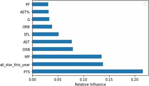
As in Figure 4 of Top 10 relative features of our classification model, it is not really surprised that the most relative feature is total points made in this season are around 0.21. It is expected that best players from each team are more likely to be the primary scorer. Being All-Star player in this year is also a significant indicator for being All-Star player next year. Total minutes played – MP has a critical role in both objectives’ models with relative influences ranking third for both cases.

Figure 4. Top 10 Relative features for final classification model by traditional machine learning.

5. Deep learning method and results

5.1. Method

Along with traditional ML, Deep Neutral Network (DNN) was implemented to forecast the performance of NBA basketball layers. Unlike traditional ML models, such as RF and KNN, finding a right NN architecture and fine-tuned hyperparameter set are difficult due to the large possible number of DNN configurations. In this study, three NN models for regression and three for classification were built, 2-layers, 3-layers, and 3-layers with more neural nodes. The best results in each group were selected to determine the difference in performance for this particular dataset between the traditional ML and modern ML (Deep Learning).

Due to a significant imbalance in the dataset, models were fit using large batch size of 512. This would ensure that each batch has a chance containing the rare cases (high achievement basketball players). This is particularly important for classification models as the classifiers would likely miss the special cases’ to learn from when the batch size was too small.

In regression models, Mean Squared Error (MSE) was selected to evaluate the performance of the models. For activation function and optimizer, ReLu and Adam were used. Optimization learning rate for Adam was left at default value, learning_rate = 0.001.

In classification, the 2-layer and 3-layer NN configuration had similar structures as NN is used in regression models. Accuracy, Precision, Recall and AUC (Area Under the ROC Curve) metrics were used to evaluate classifiers. For 3-layer NN (model_2), a special NN structure known as Autoencoder layer was built on the top of the 3-layer NN to reconstruct the raw input data. These layers would act as unsupervised features extracting to help hidden layers learn the data better.

5.2. Results

5.2.1. Regression analysis

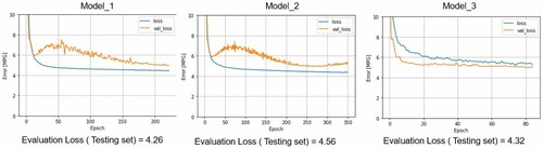
This appeared that the 3-layers with complex activation nodes (model_3) showed the best performance result. Comparing the 3 charts (Figure 5), the Model_3 had the lowest validation loss value. The average loss (MSE) value on testing set was around 4.32 which is nearly 0.4 smaller compared to Model_1 and Model_2. While the gap between validation loss and training loss in Model_3 was small, the training loss curve had a larger value compared to the validation loss. This indicated some under-fitting happening in Model_3. The loss value curve showed the loss (training and validation) decreased to stable significant faster than the others. Early stopping function was applied when epochs reached 50. The stopping function is used to stop training model running when there are no signs of improvement in training process.

Figure 5. Loss function results for train and valid data and evaluation loss for test data from each candidate deep learning model.

5.2.2. Classification analysis

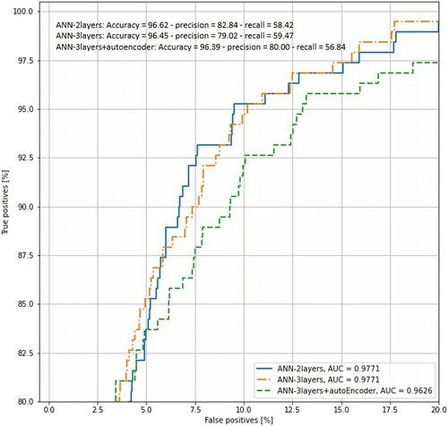
Three classifications had very prominent result for this imbalance dataset. The AUC (Area Under the Curve) suggested all models were capable of predicting between positive and negative cases of ‘All Start Next Year’. ANN-2layers (Classi_model_1) and ANN-3layers (Classi_model_2) had nearly the same performance. Both models performed slightly better compared to ANN-3layers + autoencoder (Classi_model_3) (Figure 6).

Figure 6. ROC curve for train data from each candidate deep learning model.

The average prediction accuracy was above 96%. Average Classification Classi_model_1 and Classi_model_2 achieved over 80% precision rate. The loss curve value showed the models were fitting well, the training and validation loss curves were closed together in all 3 models (Figure 7).

Figure 7. Loss function results for train and valid data and confusion matrix results for test data from each candidate deep learning model.

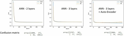
Overall, Classi_model_1 appeared the most suitable NN classifier candidate for detecting All Start Next Year. Based on the Classi_model_3’s confusion matrix table, out of 190 actual ‘All Start Next Year’ cases, the model was able to predicted correctly 108 cases – a 76% chance of predicting ‘All Start Next Year’ correctly (Figure 7).

6. Limitations

As a team-oriented sport, there are some other factors influencing the players’ performance and popularity: team’s tactical style, coach decision, team chemistry … , which are not included in our study and would be more accessible to study to improve the models in the future. Although NBA season includes 2 periods: regular season and playoff when the best 16 teams in a regular season compete for the championship, all data used in our study are regular season’s stats. Thus, these ML and DL models may not be suitable to predict players’ performance in playoff and the effect of prior playoff performance on players’ popularity is also overlooked in this study. Popularity is also affected by external non-sporting factors, such as celebrity status in media, charisma, social media compared to the pure quality of the game (Adler, 1985). As these factors are perceived distinctively by public in terms of time and geography, it is a complicated issue and further research is needed.

7. Conclusion

Machine learning can give many advantages in Sport domain with its capability to predict the future outcomes, which can be seen through our study’s results: RMSE of 2.1969 and MAE of 1.6465 for Regression Analysis, Recall of 0.9368 and ROC AUC of 0.9152 for Classification Analysis. Moreover, our result is consistent with many prior studies proving the better capability of Under-Sampling technique compared to Over-Sampling on solving Imbalanced Data issue. Additional, Deep Learning is also applied for both Regression and Classification Analysis. Our study showed Deep Learning’s performance is not as good as traditional Machine Learning’s. It is justified that our data are relatively small-scale and structured with a few predictor variables. Thus, it limited Deep Learning’s efficiency on Big Data, which is universally recognized in Computer Vision and Natural Language Processing fields. Because our study used intensively pure basketball statistics for models, it possibly neglects the critical influence of external factors on popularity. Thus, it is suggested further studies in this domain with more external variables would improve the predictive ability and provide more comprehensive understanding about the degree of importance of different factors.

Disclosure statement

No potential conflict of interest was reported by the author(s).

Additional information

Notes on contributors

Nguyen Hoang Nguyen

Nguyen Hoang Nguyen is Senior Business Intelligence at ShopeePay, Vietnam (Sea Group – Singapore) since May 2021. He received Master degree of Data Science at Texas Tech University in 2019. His research interest is business intelligence based on big data, machine learning and data privacy. Recently, he focuses on developing intelligent marketing forecasting systems by using machine learning and deep learning methodologies.

Duy Thien An Nguyen

Duy Thien An Nguyen is taking Master by Research at University of Southern Queensland since 2021. He received Master degree of Data Science at University of Southern Queensland in 2021. His research interest is the application of data science in different industries. He is focusing on developing a data ecosystem for the development of an automated trading platform.

Bingkun Ma

Bingkun Ma received Master degree of Data Science at Texas Tech University in 2019. His research interest is the application of data science in finance and accounting.

Jiang Hu

Jiang Hu received PhD degree at Texas Tech University.

References

- Adler, M. (1985). Stardom and talent. American Economic Review, 75(1), 208–212.
- Apostolou, K., & Tjortjis, C. (2019). Sports Analytics algorithms for performance prediction. In 10th International Conference on Information, Intelligence, Systems and Applications (IISA), PATRAS, Greece. https://doi.org/https://doi.org/10.1109/IISA.2019.8900754.
- Batista, G. E. A. P. A., Prati, R. C., & Monard, M. C. (2004). A study of the behavior of several methods for balancingmachine learning training data. ACM SIGKDD Explorations Newsletter, 6(1), 20–29. https://doi.org/https://doi.org/10.1145/1007730.1007735
- Batuwita, R., & Palade, V. (2009). Micropred: Effective classification of pre-miRNAs for human miRNA gene prediction. Bioinformatics (Oxford, England), 25(8), 989–995. https://doi.org/10.1093/bioinformatics/btp107
- Berri, D. J., & Schmidt, M. B. (2006). On the road with the National Basketball Association’s superstar externality. Journal of Sports Economics, 7(4), 347–358. https://doi.org/https://doi.org/10.1177/1527002505275094
- Blagus, R., & Lusa, L. (2013). SMOTE for high-dimensional class-imbalanced data. BMC Bioin-Formatics, 14(1), 106. https://doi.org/https://doi.org/10.1186/1471-2105-14-106
- Boser, B. E., Guyon, I. M., & Vapnik, V. N. (1992, July 27 - 29). A training algorithm for optimal margin classifiers. Proceedings of the 5th Annual Workshop on Computational Learning Theory (COLT’92), Pittsburgh.
- Bottou, L., & Bousquet, O. (2012). The tradeoffs of large scale learning. In S. Sra, S. Nowozin, & S. J. Wright (Eds.), Optimization for machine learning (pp. 351–368). MIT Press. ISBN 978-0-262-01646-9.
- Breiman, L. (1996). Bagging predictors. Machine Learning, 24, 123–140. https://doi.org/https://doi.org/10.1007/BF00058655
- Bromley, J., Bentz, J. W., Bottou, L., Guyon, I., Lecun, Y., Moore, C., Säckinger, E., & Shah, R. (1993). Signature verification using a “siamese” time delay neural network. International Journal of Pattern Recognition and Artificial Intelligence, 7(04), 669–688.
- Brownlee, J. (2016). XGBoost with Python: Gradient boosted trees with XGBoost and Scikit-Learn (pp. 10–11). Machine Learning Mastery.
- Burges, Christopher J. C. (1998). Data Mining and Knowledge Discovery, 2(2), 121–167. https://doi.org/https://doi.org/10.1023/A:1009715923555
- Chawla, N. V., Bowyer, K. W., Hall, L. O., & Kegelmeyer, W. P. (2002). SMOTE: Synthetic minority over-sampling technique. Journal of Artificial Intelligence Research, 16, 321–357. https://doi.org/https://doi.org/10.1613/jair.953
- Chawla, N. V., Japkowicz, N., & Kolcz, A. (2004). Special issue learning imbalanced datasets, SIGKDD Explor. Newsl, 6, 1–6. https://doi.org/https://doi.org/10.1145/1007730.1007733
- Chen, C., Liaw, A., & Breiman, L. (2004). Using random forest to learn imbalanced data. University of California. 110: pp.1–12.
- Cieslak, D. A., Chawla, N. W., & Striegel, A. (2006). Combating imbalance in network intrusion datasets. In Proceedings of the IEEE International Conference on Granular Computing, Atlanta, Georgia, USA.
- Colet, E., & Parker, J. (1997). Advanced scout: Data mining and knowledge discovery in NBA data. Data Mining and Knowledge Discovery, 1(1), 121–125. https://doi.org/https://doi.org/10.1023/A:1009782106822
- Drucker, H., Burges, C. J., Kaufman, L., Smola, A., & Vapnik, V. (1997). Support vector regression machines. Advances in Neural Information Processing Systems, 9, 155–161.
- Drummond, C., & Robert, C. H. (2003). C4. 5, class imbalance, and cost sensitivity: Why under-sampling beats over-sampling. In Workshop on Learning from Imbalanced Datasets II, 11. Citeseer.
- Fallahi, A., & Jafari, S. (2011). An expert system for detection of breast cancer using data pre-processing and Bayesian network. International Journal Advanced Science Technology, 34, 65–70.
- Freund, Y., & Schapire, R. E. (1997). A decision-theoretic generalization of on-line learning and an application to boosting. Journal of Computer and System Sciences, 55(1), 119–139. https://doi.org/https://doi.org/10.1006/jcss.1997.1504
- Galar, M., Fernandez, A., Barrenechea, E., Bustince, H., & Herrera, F. (2011). A review on ensembles for the class imbalance problem: Bagging-, boosting-, and hybrid-based approaches. IEEE Transactions on systems, Man, and Cybernetics. Part C (Applications and Reviews), 42(4), 463–484. https://doi.org/https://doi.org/10.1109/TSMCC.2011.2161285
- Guo, H., & Herna, L. V. (2004). Learning from imbalanced data sets with boosting and data generation. ACM Sigkdd Explorations Newsletter, 6(1), 30–39. https://doi.org/https://doi.org/10.1145/1007730.1007736
- He, H., & Garcia, E. A. (2009). Learning from imbalanced data. IEEE Transactions on Knowledge and Data Engineering, 21(9), 1263–1284. https://doi.org/https://doi.org/10.1109/TKDE.2008.239
- Hosmer, D. W., & Lemeshow, S. (2000). Applied logistic regression. Wiley-Interscience.
- Hothorn, T., Hornik, K., & Zeileis, A. (2006). Unbiased recursive partitioning: A conditional inference framework. Journal of Computational and Graphical Statistics, 15(3), 651–674. https://doi.org/https://doi.org/10.1198/106186006X133933
- Hulse, J. V., Khoshgoftaar, T. M., & Napolitano, A. (2007). Experimental perspectives on learning from imbalanced data. In Proceedings of the 24th International Conference on Machine Learning (pp. 935–942). Oregon State University.
- Humphreys, B. R., & Johnson, C. (2020). The effect of superstars on game attendance: Evidence from the NBA. Journal of Sports Economics, 21(2), 152–175. https://doi.org/https://doi.org/10.1177/1527002519885441
- Kahn, J. (2003). Neural network prediction of NFL Football Games.
- Kubat, M., & Matwin, S. (1997). Addressing the curse of imbalanced data sets: One-sided sampling. In Proceedings of the 14th International Conference on Machine Learning (pp. 179–186). Morgan Kaufmann.
- Langley, P., Iba, W., & Thompson, K.. (1992). An analysis of Bayesian classifiers. The Tenth National Conference on Artificial Intelligence, 223–228. AAAI Press. https://doi.org/https://doi.org/10.5555/1867135.1867170
- Leung, C. K., & Joseph, K. W.. (2014). Sports data mining: Predicting results for the college football games. Procedia Computer Science, 35, 710–719. https://doi.org/https://doi.org/10.1016/j.procs.2014.08.153
- Ling, C., & Li, C. (1998). Data mining for direct marketing problems and solutions (1998).
- Madhavan, V. (2016). Predicting NBA game outcomes with hidden Markov models. Berkeley University.
- Maher, M. J. (1982). Modelling association football scores. Statistica Neerlandica, 36(3), 109–118. https://doi.org/https://doi.org/10.1111/j.1467-9574.1982.tb00782.x
- Marcus, G. (2018). Deep learning: A critical appraisal. arXiv preprint arXiv, 1801.00631.
- McCabe, A., & Trevathan, J.. (2008). Artificial intelligence in sports prediction. Fifth International Conference on Information Technology: New Generations (itng 2008), 1194–1197. https://doi.org/https://doi.org/10.1109/ITNG.2008.203
- Miljković, D., Gajić, L., Kovačević, A., & Konjović, Z. (2010). The use of data mining for basketball matches outcomes prediction. In IEEE 8th International Symposium on Intelligent Systems and Informatics, Subotica. https://doi.org/https://doi.org/10.1109/SISY.2010.5647440.
- Nguyen, N., Ma, B., & Hu, J. (2020). Predicting National Basketball Association players performance and popularity: A data mining approach. Computational Collective Intelligence. ICCCI 2020, Da Nang, Nov 28 - Dec 3. Lecture Notes in Computer Science, vol 12496. Springer, Cham. https://doi.org/https://doi.org/10.1007/978-3-030-63007-2_23.
- Pifer, N. D., Mak, J., Bae, W., & Zhang, J. (2015). Examining the relationship between star player characteristics and brand equity in professional sport teams. Marketing Management Journal, 25, 88–106.
- Releases, Forbes Press. (2019, February 6). Forbes releases 21st annual NBA team valuations. Forbes. Retrieved May 26, 2021, from www.forbes.com/sites/forbespr/2019/02/06/forbes-releases-21st-annual-nba-team-valuations/?sh=72543d3511a7
- Rotshtein, P., Posner, M., & Rakityanskaya, A. B. (2015). Football predictions based on a fuzzy model with genetic and neural tuning. Cybernetics and Systems Analysis, 41(4). https://doi.org/https://doi.org/10.1007/s10559-005-0098-4
- Schwenk, H., & Bengio, Y.. (1997). Artificial Neural Networks — ICANN'97. ICANN 1997. Lecture Notes in Computer Science, Vol. 1327. Berlin: Springer. https://doi.org/https://doi.org/10.1007/BFb0020278
- Thabtah, F., Zhang, L., & Abdelhamid, N. (2019). NBA game result prediction using feature analysis and machine learning. Annals of Data Science, 6(1), 103. https://doi.org/https://doi.org/10.1007/s40745-018-00189-x
- Tichy, W. (2016). Changing the Game: ‘Dr. Dave’ Schrader.
- Wirth, R., & Hipp, J. (2000, April). CRISP-DM: Towards a standard process model for data mining. In Proceedings of the 4th International Conference on the Practical Applications of Knowledge Discovery and Data Mining, Citeseer.
- Yan, X., & Su, X. (2009). Linear regression analysis: Theory and computing (pp. 2–3). https://doi.org/https://doi.org/10.1142/6986
- Yanofsky, N. (2015). Probably approximately correct: Nature’s algorithms for learning and prospering in a complex world. Common Knowledge, 21(2), 340–340. https://doi.org/https://doi.org/10.1215/0961754X-2872666
- Zimmermann, A., Moorthy, S., & Shi, Z. (2013). Predicting college basketball match outcomes using machine learning techniques: some results and lessons learned. arXiv preprint arXiv:1310.3607.
- Zuccolotto, P., Manisera, M., & Sandri, M. (2018). Big data analytics for modelling scoring probability in basketball: The effect of shooting under high-pressure conditions. International Journal of Sports Science & Coaching, 13(4), 569–589. https://doi.org/https://doi.org/10.1177/1747954117737492