Multi-category diagnostic accuracy based on logistic regression

ABSTRACT

We provide a detailed review for the statistical analysis of diagnostic accuracy in a multi-category classification task. For qualitative response variables with more than two categories, many traditional accuracy measures such as sensitivity, specificity and area under the ROC curve are no longer applicable. In recent literature, new diagnostic accuracy measures are introduced in medical research studies. In this paper, important statistical concepts for multi-category classification accuracy are reviewed and their utilities are demonstrated with real medical examples. We offer problem-based R code to illustrate how to perform these statistical computations step by step. We expect such analysis tools will become more familiar to practitioners and receive broader applications in biostatistics. Our program can be adapted to many classifiers among which logistic regression may be the most popular approach. We thus base our discussion and illustration completely on the logistic regression in this paper.

KEYWORDS:

• Hypervolume under the ROC manifold
• multi-category classification
• correct classification probability
• net reclassification improvement
• integrated discrimination improvement
• marker evaluation
• R software

1. Introduction

Statistical classification is needed in fields such as economics, computer science, meteorology and biology. Particularly in clinical studies, the accurate diagnosis of a patient's condition is crucial for proper treatment. An assessment of these conditions and evaluation of the prognosis of patients with disease can be achieved by analysing clinical and laboratory data. For two-category classification (e.g., diseased and non-diseased conditions), receiver operating characteristic (ROC) curves and the area under the ROC curve (AUC) measure have been, for decades, the most recommended and applied methods for evaluating the accuracy of numerical diagnostic tests (Pepe, 2003; Zhou, Obuchowski, & McClish, 2002).

Medical decision-making sometimes may involve more than two categories. For example, cognitive function declines from normal function, to mild impairment, to severe impairment and/or dementia. Another example is the stage of cancer progression at the time of detection, from localised cancer through distant metastases already present. We need statistical methods for the assessment of diagnostic accuracy when the true disease status is multi-category. Accuracy measures for binary classification are not applicable and their extensions must follow a rigorous methodology construction.

Let us first consider three practical examples from recent medical studies. They will be analysed using methods introduced in this tutorial.

Example 1.1 (Liver Cancer):

In Ressom et al. (2007, 2008), 203 participants from Cairo, Egypt, were investigated, where 73 were hepatocellular carcinoma (denoted by HC) cases, 52 were patients with chronic liver disease (denoted by QC), and 78 were healthy individuals (denoted by NC). The data contain intensity measurements of hundreds of protein segments or peptides, also called peaks. Each peak can be regarded as a diagnostic test for differentiating the subjects from the three distinctive classes. A set of 484 peaks after extensive preprocessing of the raw data are available from the authors’ website. We were interested in studying the diagnostic accuracy of these peaks, and identifying those peaks with the highest discriminatory ability.

Example 1.2 (Synovitis):

In Ogdie et al. (2010) and Beffa et al. (2013), immunohistochemical synovial tissue biomarkers are used to classify arthropathies, study their pathogenesis and to measure disease activity in clinical trials. The markers are common inflammatory cells (including subintimal CD15, CD68, CD3, CD20, CD38 and lining CD68), proliferating cells (Ki-67) and blood vessels (von Willebrand factor, vWF). The disease status for all patients included chronic septic arthritis (SeA), early undifferentiated arthritis (Early), rheumatoid arthritis (RA), osteoarthritis (OA), noninflammatory orthopedic arthropathies (Orth.A) and normal synovium. Data from six categories were collected with sample sizes 15 (normal), 26 (OA), 6 (Orth.A), 10 (Early), 11 (SeA) and 25 (RA), respectively. Placing an individual into any wrong category may result in adverse consequences. The accuracy of the gene should ideally be reflected by how often the gene correctly classifies all six categories.

Example 1.3 (Leukemia):

Golub et al. (1999) analysed a leukemia data-set using micro-array gene expression. The data included three types of acute leukemias: acute lymphoblastic leukemia arising from T-cells (ALL T-cell), acute lymphoblastic leukemia arising from B-cells (ALL B-cell) and acute myeloid leukemia (AML). The data-set contains 8 ALL T-cell samples, 19 ALL B-cell samples and 11 AML samples. Each sample contains 3916 gene expression values obtained from Affymetrix high-density oligonucleotide micro-arrays. The data-set to be analysed is downloaded from http://www.broad.mit.edu/cgi-bin/cancer/datasets.cgi.

In all the above examples, we need to statistically assess the diagnostic accuracy of biomarkers or medical tests for multi-category classification. This topic has now been thoroughly studied. In fact, the usual 0–1 error rate and ROC analysis for binary classification can be extended for multi-category classification. In this tutorial, we first review familiar classification devices and decision-making rules for multi-category problem in Section 2 and then summarise the major multi-category diagnostic accuracy measures in Section 3. Many accuracy measures are constructed from the correct classification probabilities (CCP) for individual categories. These quantities themselves may be important and provide category-specific assessment on the classification performance. However, to summarise the overall accuracy with a single diagnostic accuracy index, we usually invoke the concept of ROC curve and produce ROC-based accuracy measures. This kind of analysis may be more relevant when we intend to examine the marker's discrimination ability as a whole over all classes. Throughout this paper, we do not assume that the categories are ordered. The distinction between nominal and ordinal categorical variables does not affect the statistical procedure for the evaluation of diagnostic accuracy. The methods presented in this paper can be straightforwardly adopted to deal with ordinal multi-category problems.

When information of new markers becomes available, investigators may incorporate such markers in their classification models and improve the diagnostic accuracy. How to quantitatively assess the improvement is of interest to biostatisticians. Two new metrics, the net reclassification improvement (NRI) and the itegrated discrimination improvement (IDI), are proposed in the literature (Pencina, D’Agostino Sr, D’Agostino Jr, & Vasan, 2008) and enjoy wide acceptance in medical practice. Their formulation for multi-category classification has also been developed for medical applications (Li, Jiang, & Fine, 2013a). We further discuss the accuracy improvement indices needed for multi-category problem in Section 4.

Real case studies are presented in Section 5 to provide an illustration. All three examples described above will be analysed with step-by-step operation instructions. We conclude in Section 6 with comments and discussions on the use of the measures.

2. Multi-category classifiers

Consider a set of predictors Ω = {X₁,… , X_p}, where (j = 1,… , p). Suppose we have a sample of n subjects with measurements {X_ij, i = 1,… , n; j = 1,… , p}. Researchers want to make use of the markers to accurately classify or predict the categorical outcome Y. Let us first recall some familiar procedures for binary classification where Y is a 0–1 variable, usually indicating the presence (Y = 1) or absence (Y = 0) of a disease condition. One of the most well-known approaches for binary classification is to regress Y on the predictors for a training sample and then evaluate the probability of class membership for the subjects based on the fitted model. Based on the risk score obtained from the model, one may then make a decision to assign the subject i to class 1 or 0 by comparing the relative magnitude of P(Y_i = 1) and P(Y_i = 0).

We now extend the aforementioned procedure for a multi-category outcome. Suppose the multi-category outcome Y takes values from . We define the binary random variable Y_m = I(Y = m) and let the prevalence for the mth category be ρ_m = E(Y_m) = P(Y = m). We consider an order-free decision-making approach which automatically incorporates multiple markers. Suppose a model is constructed based on a set of predictors Ω₁⊂Ω. Such a model can generate a probability vector … , for each subject such that =1. Each component in the vector indicates the predicted probability of the mth class membership and therefore generalises the risk score for binary regression. We may then consider the following rule:

Take-the-winner rule:

• Assign a subject to one of the M categories which corresponds to the greatest component in the M-dimentional probability vector p.

We note that when the model is fitted adequately, the subject from a particular class should be rewarded the highest probability score in that class. In a statistical analysis with a large sample size, the class probability estimates are consistent to the true class probability. The “winner” class of the risk score is thus of high agreement with the true class and subsequently we achieve a sensible classification.

Compared to other classification rules, this decision rule does not need the specification of any cut-off values and is more flexible and realistic. This rule has been widely used in the multi-category classification (Li et al., 2013a). In a binary classification problem, using this rule we assign the ith subject to class 1 if P(Y_i = 1) > P(Y_i = 0) and to class 0 otherwise.

There are abundant research development to compute the vectors of class probability estimates. Among them, the simplest method perhaps is the multi-nomial logistic regression model by using the multiple-category indicator variable as the response and using the diagnostic tests involved in Ω₁ as the predictor. From the fitted model, we may then evaluate the model-based prediction on the probability scale. We will use logistic regression as the working classifier in this paper. More details for fitting this model can be found in Appendix of this paper. In addition to multi-nomial logistic regression analysis, one can also use other well-known machine learning methods or classifiers such as the classification trees (Breiman, Friedman, Olshen, & Stone, 1984) and the support vector machines (SVM) (Vapnik, 1998) with outputs being probability estimates.

3. Diagnostic accuracy

3.1. Correct classification probability and R²

For the simplicity of presentation, we still consider a fixed model with a set of covariates Ω₁. Following the take-the-winner rule in the preceding section, a correct decision is obtained if a subject from Class m has the highest predicted probability for the mth class. The correct classification probability (CCP) for the mth category is thus given by (1) In a binary classification M = 2, the two CCPs are the well-known sensitivity and specificity (Pepe, 2003; Zhou et al., 2002). The event defining the CCP is equivalent to the zero–one scoring rule which rewards a probabilistic forecast if the mode of the predictive distribution materialises (Gneiting & Raftery, 2007; Toth, Zhu, & Marchok, 2001).

The CCP definitions (1(1) ) are based on events of successful classification and can be easily estimated by using empirical distribution estimates. These category-specific accuracy measures, however, do not provide an overall assessment of the classification accuracy. When ranking different diagnostic tests for their discrimination ability, we need a single measure to quantify the overall accuracy of the marker or the combination of markers. A simple weighted average of the class-specific CCP yields the overall CCP: (2) where the weight ρ_m is usually taken to be the class prevalence. CCP heavily depends on the class prevalences (Allwein, Schapire, & Singer, 2000) and hence is not comparable across populations. This contrasts with ROC-based measures to be introduced in the next subsection, which are prevalence independent.

Other model-based statistics such as log-likelihood functions, deviance functions and some significance tests along with their p-values are sometimes reported as performance measures for multi-class problems. These quantities may be helpful to evaluate the correlation between the polychotomous outcome and the markers but do not necessarily lead to classification accuracy.

Another popular index derived from a fitted regression model is the model R² (Cox & Wermuth, 1992; Hu, Palta, & Shao, 2006; Menard, 2000; Tjur, 2009). The interpretation and computation of R², also called a coefficient of determination, has been well known for binary logistic regression models. Simply speaking, the value of R² is the fraction of the total variation explained by the model. For linear regression models, R² is closely related to the correlation coefficient and the ANOVA F-test, while for binary regression, it is closely connected to the probabilities of correct classification.

We consider the definition of R² for multi-category classification. Specifically, for the mth category, the R² value for a model is defined to be (3) The second equality follows because . The overall accuracy may be computed as a weighted sum of the R² values as (4) where w_m are properly chosen weights.

3.2. ROC analysis

Recall in binary classification, we need one cut-off c for the disease probability p to define the separation of disease-present subjects from disease-absent subjects. For example, when fixing c = 0.5, we claim the subject as being diseased if his corresponding p > 0.5 and being normal if p ≤ 0.5. Varying the threshold value c from 0 to 1, we obtain a set of sensitivity and specificity pairs. When displaying the pairs in a two-dimensional plane, the so-called ROC curve shows clearly the trade-off between sensitivity and specificity. The AUC represents the overall accuracy of the marker(s).

The idea can be straightforwardly extended to multi-category classification. For M = 3, one can obtain the probability assessment vector p = (p₁, p₂, p₃) for a subject and choose two cut-off values c₁ and c₂ to define the classification rule as follows:

Thresholding rule:

• If p₁ > c₁, assign the subject to Class I;

• Otherwise if p₂ > c₂, assign the subject to Class II;

• Otherwise assign the subject to Class III.

We remark that this rule is usually only applicable for ordered categories and is not as widely used as the take-the-winner rule introduced in the preceding section. We adopt the thresholding rule only as a conceptual tool in this paper since it easily lends support to the multidimensional ROC construction. The following accuracy measures are equally applicable to ordered and unordered classes.

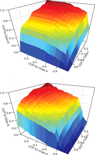
Under the above thresholding rule, the cut-off-specific CCPs may be computed as When varying the threshold values (c₁, c₂) in [0, 1] × [0, 1], we may plot the triples CCP₁(c₁, c₂), CCP₂(c₁, c₂) and CCP₃(c₁, c₂) in the three-dimensional space and obtain an ROC surface. Figure 1 provides two examples of the ROC surface based on the liver cancer data-set. The volume under the ROC surface (VUS) becomes a meaningful summary measure. More generally, we may consider higher dimension where M ≥ 3. In mathematics, a multidimensional surface is termed manifold. We may construct multidimensional ROC manifold (CCP₁,… , CCP_M) and compute the hypervolume under the multidimensional ROC manifold (HUM) as an extension of AUC to evaluate the overall classification accuracy for any biomarker in a multi-class problem.

Figure 1. The estimated ROC surface for peak 3 (top) and peak 4 (bottom) in liver cancer example.

Scurfield (1996) presented a rigorous extension of two-class ROC to a finite number of classes and generalised the two-class AUC via an information theoretic derivation. This foundational work focused primarily on the higher dimensional ROC framework at the population level. No inferential procedure was proposed for use with randomly sampled data, and empirical results were not presented. Mossman (1999) introduced the concept of three-way ROC analysis into medical decision-making. Heckerling (2001) discussed parametric estimation of three-dimensional ROC measures under the joint normality assumption. Dreiseiltl, Ohno-machado, and Binder (2000) derived variance estimators for the VUS estimator and provided a hypothesis test method. Nakas and Yiannoutsos (2004) considered the estimation of HUM for the ordered three-class problem. Li and Fine (2008) further proposed the estimation of HUM for unordered classification by following the probabilistic interpretation and applied HUM as a model selection criterion in micro-array studies. Li and Zhou (2009) discussed the estimation of three-dimensional ROC surfaces. Xiong et al. (2006) also provided a test procedure to compare HUM for three ordinal classes. Zhang and Li (2011) combined multiple markers to improve diagnostic accuracy for three-way ROC analysis. Most recently, Shiu and Gatsonis (2012) developed a semi-parametric model for non-binary classification.

HUM has an interpretation akin to AUC where a large HUM value indicates a high classification accuracy (Dreiseiltl et al., 2000). Suppose X_m is the marker value for a randomly selected subject from Class m, i.e., Y_m = m. HUM may be defined by (5) where (m₁, m₂,… , m_M) is a permutation of (1, 2,… , M) such that (5(5) ) is the greatest among all possible permutations. This is the probability of correctly sorting M subjects each from one of the M categories. When the categories are naturally ordinal, the permutation may be known exactly. Otherwise the numerical value of X may indicate the correct permutation order among the M classes. For example, the gene expression values for one type of cancer patient may tend to be greater than those for another type of cancer even though there is no natural order for the two types of diseases. However, this numerical order has to be discovered from the data and cannot be given a priori. In fact, for M = 3, Scurfield (1996) introduced six HUM measures which correspond to six different triple-comparison probabilities where (m₁, m₂, m₃) is a permutation of (1, 2, 3). Among the six HUMs, only the largest one is a reasonable measure of the accuracy of the test (Nakas & Alonzo, 2007). For a general M-category problem, we need to evaluate M! such HUM measures to identify the largest HUM. When X_m, m = 1,… , M, are from the normal distribution, it was proved in Li, Chow, Wong, and Wong (2014) that the order of the mean E(X_m) can prescribe the definition of HUM. In this special parametric case, the form of HUM can be quickly determined. Alternatively, one has to exhaustively compute all possible probabilities to arrive at the correct HUM definition. Following this idea, the HUM package was implemented in R by Novoselova et al. (in press). The auxiliary functions CalcGene and CalcROC of the HUM package are written in the C++ language and are integrated in R through the Rcpp package. These functions improve computational efficiency and shorten the computational time.

Another HUM calculation method for unordered categories has been proposed in Li and Fine (2008). The event described in the definition (5(5) ) may be extended to the event of simultaneously correctly classifying M subjects each from one of the M categories. The correct classification may not need to be established by the inequality of X and can be established by a slightly more complicated geometrical rule.

Consider M subjects, each randomly drawn from one of the M classes, with probability ratings p⁽¹⁾, p⁽²⁾,… , p^(M), respectively. Each probability rating p^(m) is a vector (E_m1, E_m2,… , E_mM), where E_m1, E_m2,… , E_mM > 0 and E_m1 + E_m2 + ⋅⋅⋅ + E_mM = 1. Each component E_mk in the vector indicates the likelihood that the mth subject is from the kth category. In practice, the probability assessment vectors can be indirectly derived from the continuous diagnostic test. The simplest way to generate such vectors is to fit a multi-nomial logistic regression model. Alternatively, one can choose multi-category SVM techniques or classification trees (Breiman et al., 1984), among many other classifiers documented in the literature.

Let v_m (m = 1, 2,… , M) be an M-dimensional vector whose elements are all 0 except that the mth element equals 1. Now we consider the following classification rule based on the probability assessment vectors of the M subjects: assign subjects to class k₁, k₂,… , k_M such that is minimised among all possible assignments k₁ ≠ ⋅⋅⋅ ≠ k_M, where ‖·‖ is the Euclidean distance. We may notice that the distance displayed above is a direct generalisation of the Brier score widely adopted as classification decision rules (Gneiting & Raftery, 2007; Selten, 1998). Let CR(p⁽¹⁾, p⁽²⁾,… , p^(M)) be 1 if all M subjects are classified correctly, and 0 otherwise. The alternative definition of HUM is then given by (6) according to its probabilistic interpretation. We note that (6(6) ) is mathematically equivalent to (5(5) ). A heuristic proof of the equivalence can be found in Li and Fine (2008).

The calculation of HUM (6(6) ) for unordered multi-category outcomes with M = 3 and M = 4 has been implemented in an R program, and the code is freely downloadable from the following web-site http://www.stat.nus.edu.sg/∼stalj.

Users may prepare data in the right format and paste the code in R to obtain the HUM values. It is quite unusual to examine M > 4 classes in medical research studies. The R package HUM may allow M = 5 or 6 for such special classification problems.

The inference procedure for HUM has been discussed in Nakas and Yiannoutsos (2004) for ordered polychotomous responses and Li and Fine (2008) for unordered polychotomous responses. Though variance formula based on U-statistic theory are provided for HUM, it may be easier for practitioners to use the resampling approach. Simulation studies in Li and Fine (2008) suggest the coverage of bootstrap confidence intervals for HUM is in general satisfactory.

3.3. Other accuracy summary measures

We next consider a few other accuracy summary measures that have been used in medicine.

3.3.1. Pairwise AUC

Because of the wide acceptance of the ROC curve and the AUC statistic, some practitioners may choose to produce similar results and consider pairwise ROC curves and pairwise AUCs (Hand & Till, 2001; Obuchowski, 2005). There are two possible methods to generate pairwise summary measures. The first method is one-versus-rest. One can construct M binary classifiers to differentiate class m (positive) from all other classes (negative), m = 1,… , M. For each classifier, we may produce the familiar ROC curve and compute its AUC. This would result in M ROC curves and M AUC values which indicate how often individual classes may be differentiated from the rest of classes. The second method is one-versus-one. One can construct binary classifiers to differentiate pairs of classes. For each pair, we may produce the familiar ROC curve and compute its AUC. This would result in ROC curves and AUC values which indicate how often two classes are differentiated from each other. These measures may be helpful to investigate individual classes but do not easily lend support to rank markers for their overall discrimination ability. In the numerical analysis of Li and Fine (2008), a marker may have large pairwise AUC values for some classes but poor pairwise AUC values for others. It is thus not straightforward to conclude the discrimination strength of the marker.

3.3.2. Umbrella volume

For three-class problems, some authors (Alonzo & Nakas, 2007; Alonzo, Nakas, Yiannoutsos, & Bucher, 2009; Nakas & Alonzo, 2007) proposed an umbrella volume defined as P(X₁ < X₂ > X₃) or P(X₁ > X₂ < X₃) for three markers randomly selected from the three classes. This measure, similar to pairwise AUC, only quantifies how often Class II is different from the other two classes and does not offer any information on discrimination ability between Class I and Class III. It is less meaningful than the HUM when the goal is to assess the overall accuracy among all categories. Furthermore, it is not easy to extend the umbrella definition for M > 3.

3.3.3. Generalised Youden's index

Youden's index for binary classification has also been extended to multi-category classification (Nakas, Alonzo, & Yiannoutsos, 2010; Nakas, Dalrymple-Alford, Anderson, & Alonzo, 2012) and some authors (Luo & Xiong, 2013; Nakas et al., 2010) proposed to use the generalised Youden's index to seek optimal cut-off values for multi-category diagnostic tests under the thresholding classification rule. For a three-class problem, the Youden's index is given by (7) This measure is sensible when the categorical outcome is ordinal or permits a natural order among the categories. The numerical optimisation to find out the cut-off values will become challenging when the number of categories increases.

3.3.4. Misclassification

Many authors prefer reporting misclassification probability (MCP) over CCP in their computation (e.g., Delaigle & Hall, 2012; Edwards & Metz, 2006; Koltchinskii & Panchenko, 2002; Schubert, Thorsen, & Oxley, 2011). Each category-specific MCP is simply the complement of the corresponding CCP, i.e., MCP_m = 1 − CCP_m. Furthermore, we note that in the engineer society, there have been massive research efforts to develop accuracy measures that incorporate the loss function for multi-category misclassification (Edwards & Metz, 2006; Edwards, Metz, & Kupinski, 2004; He & Frey, 2007; He, Gallas, & Frey, 2010; Schubert, Thorsen, & Oxley, 2011, among others). The resulting summary measures appear to be an expected utility value where the expectation is taken with respect to all correct and incorrect classification events. These measures require a known utility or cost assignment for individual classes and have only been discussed at the population level. There is still a lack of sample-based estimation and statistical inference procedure and consequently these measures are not easily accessible for practitioners in biomedical research.

3.3.5. Polytomous discrimination index

In an attempt to generalise HUM, Van Calster et al. (2012a, 2012b) proposed a polytomous discrimination index (PDI). To define this measure, it is also pertinent to consider the set of M subjects each randomly drawn from one of the M classes. The overall PDI value is interpreted as the probability of correctly identifying one subject among the set and we may denote it by PDI(1). The event in the definition of PDI(1) may then be considered as the union of M disjoint events of correctly identifying the subject from the mth category, m = 1,… , M. The PDI value is obtained as the average of the M category-specific PDIs. In general, when M is large, the HUM value for an individual diagnostic test may be rather small since it is usually quite difficult to use only one test to simultaneous correct identifying all M subjects in the set. On the other hand, the PDI(1) may appear much larger for the same test since the event of one correct identification has a greater chance to occur. In fact, PDI(1) for a useless marker, i.e., a random guess, attains a lower bound at 1/M which is much larger than 1/M!, the null value of HUM. Following the same manner as Van Calster et al. (2012a, 2012b), we can similarly define PDI(m) to be the probability of correctly identifying m subjects among the set of M subjects each from the M categories, 1 ≤ m ≤ M. It is straightforward to show that PDI(m₁) ≥ PDI(m₂) for m₁ < m₂ and PDI(M) is equivalent to HUM. The lower bound for PDI(m) is (M − m)!/M!, corresponding to a random guess. All of these PDI quantities may be worth investigating as alternatives to HUM. The inference methods for PDI(1) have been rigorously studied in Li, Feng, Fine, Pencina, and Van Calster (2017) and the relevant code is available from the first author's website.

4. Accuracy improvement

While ROC-based measures have been widely adopted, it has been argued by many authors (Pepe et al., 2004; Pencina et al., 2008) that such measures may not be good criteria to quantify improvements in diagnostic accuracy when the added value of a new predictor to an existing model is of interest. Such analyses are critical in the development of predictive models based on biomarkers, where the added value of markers which may be expensive to obtain must be weighed against the associated financial costs. The interpretation of the AUC provides an indirect assessment of the predictive performance of a model. Thus, the gain with a new predictor may be unclear. A related issue is that the AUC measures may be relatively insensitive to the addition of predictors in certain regions of the AUC space. To address these limitations, Pencina et al. (2008) proposed two novel criteria based on reclassification in order to directly quantify the extent to which a new predictor improves classification performance: the net reclassification improvement (NRI) and the integrated discrimination improvement (IDI). These measures have met with a widespread success in the medical literature, with many practitioners preferring their ease of interpretation versus ROC-based measures. For additional discussion of these recent developments, we refer the reader to Steyerberg et al. (2010), Pencina, D’Agostino Sr, and Steyerberg (2011), Pencina, D’Agostino Sr., and Demler (2012) and Austin and Steyerberg (2013). We note that these metrics provide different perspectives for accuracy studies and there are also critiques in the literature (see e.g., Hilden & Gerds, 2014; Kerr et al., 2014; Pepe, Feng, & Gu, 2008b). In particular, Hilden and Gerds (2014) pointed out that NRI and IDI sometimes may inflate the prognostic performance of added biomarkers and Kerr et al. (2014) argued that NRI may perform poorly under some nonlinear data-generating mechanisms. Thus users of these popular metrics should also exercise caution in practice.

We adopt the same notations in the preceding section. Now suppose more variable(s) are included in addition to the existing model and we construct a model which is based on a set of predictors Ω₂⊃Ω₁.The newly constructed model generates another probability vector … , for each subject where . Again, decision-makers may follow the take-the-winner rule and assign the subject according to the greatest value of this probability vector and the mth-category accuracy of based on Ω₂ can be quantified by (8)

The net reclassification improvement from to may be computed by (9) where w_m are positive weights for the mth category. When M = 2, the NRI quantifies the overall increase of the weighted sum of sensitivity and specificity. When equal weights are used for the two categories, NRI is simply the difference of Youden's index between the two models (Li et al., 2013a, 2013b).

The IDI can be generalised to multiple categories by noticing the connection between IDI in binary classification problems and R² (Cox & Wermuth, 1992; Menard, 2000; Tjur, 2009). The interpretation and computation of R², also called a coefficient of determination, has been discussed for binary logistic regression models. Simply speaking, the value of R² is the fraction of the total variation explained by the model. For linear regression models, R² is closely related to the correlation coefficient and the ANOVA F-test, while for binary regression, it is closely connected to the probabilities of correct classification.

Let be an M-dimensional vector with R²_m defined in (3(3) ). It has been shown in Pepe et al. (2008a) that the increase in R² for binary classification (M = 2) from model to model is equivalent to the IDI in Pencina et al. (2008). A natural adaptation of the R² definition of IDI to the multi-category set-up is (10) The multi-category IDI (10(10) ) reduces to that in Pencina et al. (2008) when M = 2 and equal weights w₁ = w₂ = 1/2 are used. This generalised version of IDI may be viewed as an extension of the familiar Brier score which is usually defined as the sum of quadratic differences (Gneiting & Raftery, 2007).

The choice of weights in the definitions of NRI and IDI may depend on the goal and design of the study. When aiming for the overall test accuracy to differentiate multiple classes, it is natural to weigh all categories equally; on the other hand, as pointed out in Pencina et al. (2011), sometimes it is useful to reward some categories with higher weights when savings associated with correct classification of such categories outweigh other categories. When cost-efficiency information is available, we can incorporate them easily in the inference for weighted NRI and IDI. There are also other practical considerations that invoke unequal weights and one can run a Bayesian prior elicitation procedure to construct reasonable weights (Li & Fine, 2010).

The estimation and statistical inference for multi-category NRI and IDI was discussed in Li et al. (2013a). The parameter estimation and variance estimation formula were implemented in R and the code is downloadable at http://www.stat.nus.edu.sg/∼stalj. Alternatively, one can choose a resampling-based approach to construct confidence intervals for NRI and IDI. An advantage of the resampling method is that the sampling variability in estimation of the probability vector may be formally accounted for in the inference.

5. Examples

In this tutorial, we used R version 3.0.3. All data-sets and computing code can be downloaded from the first author's website.

5.1. Liver cancer

We return to the liver cancer example mentioned in Section 1. The data-set was analysed in a recent mass spectrometry study for the detection of Glycan biomarkers for liver cancer (Ressom et al., 2007, 2008). The researchers investigated 202 participants from Cairo, Egypt: 73 HC, 52 QC, and 77 NC. The spectra were generated by matrix-assisted laser desorption/ionisation time-of-flight (MALDI-TOF) mass analyser (Applied Biosystems Inc., Frammingham, MA). We downloaded the full data-set from the authors’ public website and focused on a set of 484 peaks after extensive preprocessing of the raw data.

In this study, the diagnostic task involved three different categories. We were interested in assessing the diagnostic accuracy of these peaks and identified those peaks with the highest discriminatory ability. Previously, Ressom et al. (2007, 2008) conducted analysis by reducing the number of categories to frame a few pairwise two-category classification problems. Pairwise ROC curves and the AUCs were reported to investigate the differentiability between two classes (e.g., HC vs. QC). However, such AUC measures cannot summarise the overall accuracy for three categories.

A more appropriate summary measure is the HUM from multi-category ROC analysis. We have selected four representative peaks from the raw data file for this tutorial. Let us first compute the HUM value for the peak in the first row of the data-set. After the data are prepared as we have done in Appendix, we may apply the following code using the ThreeHUM function to obtain the HUM value. > ThreeHUM(y,d1) [1] 0.1680032

Recall that the null value of HUM for three-category classification is 1/3! = 1/6 = 0.1667. The accuracy of this marker is thus slightly better than a random guess, indicating the probability of correctly classifying three subjects randomly selected from the three groups is 0.1680.

For the sake of comparison, we also compute the PDI(1) value for the same marker using the ThreePDI function.

> ThreePDI(y,d1) [1] 0.6649002

This value indicates that the probability of correctly classifying one of three subjects randomly selected from the three groups is 0.6649.

Both HUM and PDI(1) suggest the first row is a weak marker and therefore not useful for the discrimination of disease classes.

In order to identify important biomarkers in this data-set, we need to repeat the above calculation for all the peaks and rank the peaks with their HUM values. We may use the following loop to compute HUM for all the 484 peaks:

hum=rep(0,4) for(i in 1:4) { hum[i]=ThreeHUM(y, ex1[i,2:203]) }

After the calculation, we may sort the HUM values and identify the peaks with high HUM values:

> shum=sort(hum,decreasing=T,index.return=T) > shum$ix [1] 3 4 2 1 > shum$x [1] 0.6268526 0.5872484 0.1717426 0.1680032

The peaks with their corresponding HUM values are shown in the above output. The peak in the third row of the data-set has the highest HUM value, suggesting that in approximately 63% of all classification jobs, this marker can correctly sort the three classes. This is almost four times the chance of a random guess. This peak can thus be deemed as a potentially useful biomarker to differentiate the three classes. The other HUM values can be interpreted similarly.

One can use a simple bootstrap procedure to compute the standard error and percentile-based confidence intervals. For example, for the third peak, we may use the following code to produce a bootstrap sample of repetition B = 250:

B=250 hum3=rep(0,B) for(b in 1:B) { id=sample(1:202,202,replace=T) hum3[b]=ThreeHUM(y[id], ex1[3,id]) }

The resulting bootstrap sample of HUM estimates is plotted in Figure 2. The boostrap standard error is 0.0404. The 95% percentile-based bootstrap confidence interval for HUM is [0.5325, 0.6897] by using the following code:

Figure 2. Bootstrap sample of HUM for the third peak in the liver cancer example.

> sd(hum3) [1] 0.04044191 > shum3=sort(hum3) > shum3[250*.025] [1] 0.5325509 > shum3[250*.975] [1] 0.6897272

To generate a nice three-dimensional view of the ROC surface, we may use a function ROCsurf downloadable at the first author's website mentioned before. We may use the following code:

> k=3; > X=ex1[k,2:74]; > Y=ex1[k,75:151]; > Z=ex1[k,152:203]; > ROCsurf(X,Y,Z);

The corresponding graph is shown in the top panel of Figure 1. By changing k=4, we may also produce the ROC surface for the fourth peak in the data-set (the bottom panel of Figure 1). These graphs can visually display the trade-off of correct classification probabilities among the three categories and help practitioners select a desirable cut-off to achieve satisfactory accuracy requirement for the classes.

Finally, if the goal is to combine multiple markers to form a more accurate classifier, we may consider using logistic regression coupled with a forward selection algorithm. Specifically, at each step, we include one more marker on top of existing markers. The stepwise results are given in the following output:

> ThreeHUM(y,cbind(ex1[3,2:203], ex1[4,2:203])) [1] 0.7290655

We may also compute CCP for the peaks after fitting a multi-nomial logistic regression. For example, for the naive model fm we fitted in Section 2, the CCP is computed to be 0.381 by the following code, indicating that roughly 40% of the subjects in the sample are correctly classified using the first two markers in the data-set:

> mean(predict(fm)==y) [1] 0.3811881

Using all four peaks in the data-set, we obtain the CCP by applying the following code, indicating that about 80% of the subjects are correctly classified using the four peaks:

> fmf=multinom(y~ ex1[1,2:203]+ ex1[2,2:203] + ex1[3,2:203]+ ex1[4,2:203]) > mean(predict(fmf)==y) [1] 0.7871287

Although the numerical values of HUM and CCP may appear similar, they contain entirely different message. The event defining CCP does not require the joint consideration of all categories and only reflect the frequency of correct identification of individual categories. One needs to be mindful interpreting these accuracy values.

5.2. Synovitis

We return to the synovitis example described in Section 1 for which we need to analyse six distinct disease categories. The data-set is available in an R package HUM and is called sim. We may load the data in R and inspect the data structure using the following code:

> library(HUM) > data(sim) > str(sim) 'data.frame': 92 obs. of 13 variables: $ SampleID : int 1 2 3 4 5 6 7 8 9 10 ... $ Disease : Factor w/ 6 levels "Early","Normal",..: 2 2 2 2 2 2 2 2 2 2 ... $ CD15 : num 0 0 0 0 0 0.05 0 0.4 0 0 ... $ CD15TIC : num 0 0 0 0 0 0.69 0 1.89 0 0 ... $ CD3 : num 10.2 4.3 3.6 0.14 2.1 1.2 2 9.8 0.2 0.5 ... $ CD3TIC : num 39.7 31 30.2 10.4 26.2 ... $ CD20 : num 2 0.38 0.3 0.1 0 2 0 0 0 0 ... $ CD20TIC : num 7.78 2.74 2.52 7.46 0 ... $ CD38 : num 0 0 0 0 0.2 0 0 0 0 0 ... $ CD38TIC : num 0 0 0 0 2.5 0 0 0 0 0 ... $ CD68subintima : num 13.5 9.2 8 1.1 5.7 4 8 11 2.15 1.34 ... $ CD68subintimaTIC: num 52.5 66.3 67.2 82.1 71.2 ... $ Total : num 25.7 13.88 11.9 1.34 8 ... > table(sim[,2]) Early Normal OA OrthArthr RA SeA 10 15 26 6 24 11

There are 92 rows corresponding to the available observations. The first column is the subject index. The second column indicates disease categories where the frequency for these categories has been shown in the above output. All the other columns are different synovial tissue biomarkers studied in Beffa et al. (2013). It it of interest to assess the diagnostic accuracy of these markers to differentiate the six disease categories.

We next consider using the R package HUM to compute the HUM values for the marker Lining. To this end, we need to specify a few optional parameters in the function CalculateHUM_Ex. The option indexF specifies the column number for the marker we wish to investigate. The option indexClass specifies the column number for the disease categories. The option allLabel is a character vector, containing the column names of the class labels, selected for the analysis. The option amountL specifies the number of categories used for the calculation of HUM. This number must be less than or equal to the distinct number of categories in the data:

> indexF=3 > indexClass=2 > allLabel=c("Normal","OA","Early","RA","SeA","OrthArthr") > amountL=6 > out=CalculateHUM_Ex(sim,indexF,indexClass,allLabel,amountL) > out$HUM Diagnosis1 Diagnosis2 Diagnosis3 Diagnosis4 Diagnosis5 Diagnosis6 3 [1,] "Normal" "OA" "Early" "RA" "SeA" "OrthArthr" "0.0866"

In this example, we select the marker CD15 from the third column of the data-set sim for the classification. For the six-category classification task, we attain the HUM value to be 0.0866 for CD15 from the above output. Recall that the null HUM value is 1/6! = 0.00138 in this case (M = 6). CD15 thus achieves an accuracy more than 60 times of the chance of a naive random guess.

The HUM package depends on the R packages gtools, rgl and Rcpp which must be installed in advance. The program does not permit missing values and one must clean the data-set to remove all missing records.

The program also allows the computation of sub-HUM values with fewer classes. For example, the possible five-category HUM values are computed below by changing the option amountL to be 5:

> out=CalculateHUM_Ex(sim,indexF,indexClass,allLabel,5) > out$HUM Diagnosis1 Diagnosis2 Diagnosis3 Diagnosis4 Diagnosis5 3 [1,] "Normal" "OA" "Early" "RA" "SeA" "0.2641" [2,] "Normal" "OA" "Early" "RA" "OrthArthr" "0.1021" [3,] "Normal" "OA" "Early" "SeA" "OrthArthr" "0.2036" [4,] "Normal" "OA" "RA" "SeA" "OrthArthr" "0.2362" [5,] "Normal" "Early" "RA" "SeA" "OrthArthr" "0.2212" [6,] "OA" "Early" "RA" "SeA" "OrthArthr" "0.1996"

Suppose we remove category OrthArthr and only investigate the other five categories. We obtain an HUM value 0.2641 for marker CD15. For five classes (M = 5), the null HUM value is 1/5! = 0.0083. We can see that all computed HUM values are much larger than the chance of a random guess. This marker is potentially useful even if we only investigate five categories. Furthermore, if one is only interested in two-category pairwise comparison, the following code can be used to generate the desired results for all pairwise AUC values:

> out=CalculateHUM_Ex(sim,indexF,indexClass,allLabel,2) > out$HUM Diagnosis1 Diagnosis2 3 [1,] "Normal" "OA" "0.7102" [2,] "Normal" "Early" "0.9933" [3,] "Normal" "RA" "1" [4,] "Normal" "SeA" "1" [5,] "Normal" "OrthArthr" "0.6111" [6,] "OA" "Early" "0.8730" [7,] "OA" "RA" "0.9599" [8,] "OA" "SeA" "1" [9,] "OA" "OrthArthr" "0.5769" [10,] "Early" "RA" "0.6083" [11,] "Early" "SeA" "0.9727" [12,] "Early" "OrthArthr" "0.8833" [13,] "RA" "SeA" "0.9242" [14,] "RA" "OrthArthr" "0.9791" [15,] "SeA" "OrthArthr" "1"

The above computation can be carried out for all other markers in this data-set. To compute HUM for all the markers, we may select their corresponding columns (3–12) in the data-set and assign that to indexF. The function CalculateHUM_Ex can then be applied to obtain HUM values simultaneously:

> indexF=seq(3,12) > out=CalculateHUM_Ex(sim,indexF,indexClass,allLabel,6) > out$HUM 3 4 5 6 7 8 [1,] "0.0866" "0.0315" "0.0698" "0.0090" "0.0183" "0.0090" 9 10 11 12 [1,] "0.0819" "0.0368" "0.1055" "0.0435"

Eyeballing the HUM list, we may notice that marker in the 11th column achieves the maximum HUM values 0.1055 among all markers. This marker may be more informative for differentiating the multiple categories of the disease.

5.3. Leukemia

We next illustrate NRI and IDI using a data-set extracted from the leukemia data (Golub et al., 1999). We consider evaluating the improvement for their ability to differentiate the three classes using two selected gene expressions. The first gene achieves a CCP value 0.7854. The R² value for this gene is 0.6364. The following is the code to input the data from an external file trains.dat and to evaluate the CCP and R². We note that CCP and R² are the parent measures for evaluating the NRI and the IDI, respectively, when the baseline is a null model:

> leuk=read.table('trains.txt', head=T) > Y=leuk[, 3] > e1=leuk[, 1:2] > rsq=RSQ( Y, e1[, 1]) > ccp=CCP( Y, e1[, 1]) > rsq [1] 0.6364734 > ccp [1] 0.7854864

We then evaluate the accuracy improvement measures by adding the second gene expression in addition to the first gene expression. The IDI for adding the second gene is 0.3906, indicating about 40% more variation can be explained by the marker. The NRI for adding the second gene is computed to be 0.2145. The following R code generates the numerical result:

> nri=NRI(Y, e1[,1], e1[,2]) > nri [1] 0.2145136 > idi=IDI(Y, e1[,1], e1[,2]) > idi [1] 0.3905515

Finally, we may also compute PDI using this sample. To compute PDI(1) for the 1184th gene, we may use our R program ThreePDI in a similar way as ThreeHUM. The resulting PDI value 0.9868 is quite high, indicating that the marker can almost always identify one category correctly. In comparison, the HUM value for this marker is slightly above 80%. The R code is given as follows:

> PDI=ThreePDI(Y, e1[,1]) > PDI [1] 0.9868421 > HUM=ThreeHUM(Y, e1[,1]) > HUM [1] 0.8116029

6. Discussion

The sample sizes in diagnostic accuracy studies must be sensibly determined at the design stage. For multi-category classification, we need to ensure that the number of subjects from every group is sufficient to allow a realistic estimation of the accuracy measures for the study population. Sometimes because of low failure rates or uneven prevalence, a medical study would yield relatively small number of subjects in some categories relative to the massive number of markers. Even though the point estimation for many diagnostic measures such as AUC, HUM, NRI and IDI might still be unbiased for small samples, their inferences would heavily rely on the large sample assumption. We thus have to weigh the statistical findings in consideration of the samples used and make a final claim with cautions.

We recommend the use of ROC analysis for mutli-category classification accuracy studies. This type of analysis extends the familiar two-category ROC analysis and lends support to the accuracy investigation by reporting a single numerical measure that summarises the overall accuracy for differentiating multiple categories. The statistical merits of this approach are well justified by previous methodological works. In addition, user-friendly programs are now available to facilitate applications in medical research.

When evaluating the accuracy improvement, it may be more appropriate to report NRI and IDI. These two metrics may find their mathematical connection with the difference between CCP and R², respectively (Li et al., 2013a, 2013b). Besides being easy to understand, they are now also widely implemented in all kinds of applications. In this paper, we mainly review nested model improvement but the development for NRI and IDI can be readily extended to non-nested model improvement as well. See Shao, Li, Fine, Wong, and Pencina (2015) for a recent discussion. In addition, Bayesian estimation for improvement statistics is also available and may be useful for inference (Huang, Li, Cheng, Cheung, & Wong, 2016).

Other measures such as pairwise AUC, individual class-specific CCP and PDI are briefly reviewed in this paper. They usually lead to indirect evaluation of the diagnostic accuracy and thus require users to report multiple values for all the categories. In comparison, ROC-based metrics lead to a direct quantification of multi-category classification accuracy. The PDI (Li et al., 2017; Van Calster et al., 2012a) may be viewed as a useful extension from HUM when the accuracy for classifying at least one group is of interest.

Acknowledgments

We thank the associate editor and the referee for helpful comments. Li's work was partially supported by National Medical Research Council in Singapore and AcRF R-155-000-174-114.

Disclosure statement

No potential conflict of interest was reported by the authors.

Additional information

Funding

Li's work was partially supported by National Medical Research Council in Singapore and AcRF R-155-000-174-114. NNSF [grant number 11371142].

Appendix

The multi-nomial logistic regression model gives class probability by a logistic-type regression equation comparing the class with a chosen baseline class, say class 1, (11) where X represents the vector of selected markers in model and . In R, fitting a multi-nomial logistic regression can be easily realised using the library nnet.

We consider the liver cancer data-set in Section 1 as an example to illustrate the calculation of membership probabilities using the logistic regression. The data is downloadable from the authors’ public website and we save the data-set in the current working directory as example1.txt. One can read the data into R using the following code:

> ex1=read.table('example1.txt',head=T) > str(ex1) 'data.frame': 4 obs. of 203 variables: $ M.Z : num 1507 1511 1512 1519 1523 ... $ HC.146 : num 239.6 120 175.1 91.6 68.4 ... $ HC.147 : num 540 104 204 186 122 ... ...

From the above output for the data frame structure, we can see that this data file contains 4 rows and 203 columns where each row corresponds to a peak. Column 1 gives the peak IDs, columns 2–74 refer to the 73 HC subjects, columns 75–151 refer to the 77 NC subjects, and column 152–203 refer to the 52 QC subjects. To conduct multi-category analysis, we may generate the three-category outcome Y using the following code:

> y=c(rep(1,73),rep(2,77),rep(3,52))

Let us select the first two markers from the data-set as predictors and use multi-nomial logistic regression to obtain the fitted probability assessment vectors:

> library(nnet) > d1=as.numeric(ex1[1,2:203]) > d2=as.numeric(ex1[2,2:203]) > fm=multinom(y~d1+d2) > pp=fm$fitted

Now the object pp stores the probability assessment vectors for all the subjects. For the first five subjects in the data-set, we obtain the following probability assessment:

> head(pp) 1 2 3 1 0.3152325 0.4630516770 0.2217159 2 0.4513196 0.1925552390 0.3561252 3 0.4716263 0.1442867970 0.3840870 4 0.4330918 0.2402745719 0.3266336 5 0.3716372 0.3785004557 0.2498624

The value in each row sums up to one, while each column corresponds to the membership probability for a particular class. For the first subject, his membership probability for class 2, 0.4630, is the highest among the three values, and this observation leads us to a decision of classifying him into the second category. Using the same rule, we classify subjects 2, 3 and 4 into the first category; we classify subject 5 into the second category. Note that the true status for all these five subjects are actually the first category and thus only subjects 2, 3 and 4 are correctly classified by using the first two markers, defined as d1 and d2 in the above code.

Another popular classifier usually adopted by researchers is the support vector machine (SVM). This learning approach is based upon the idea of maximising the margin, i.e., maximising the minimum distance from the separating hyperplane to the nearest class member. The basic SVM supports only binary classification, but extensions (Crammer & Singer, 2001; Lee, Lin, & Wahba, 2004) have been proposed to handle the multi-category classification as well. In these extensions, additional parameters and constraints are added to the optimisation problem to handle the separation of the different classes. These sophisticated methods are all implemented in R, SAS, STATA and other statistical softwares. As an illustration, we still consider the above example and use R function ksvm to obtain the SVM classification. This function is contained in package kernlab:

> library(kernlab) > fm2=ksvm(y ~ d1+d2, prob.model = TRUE,type = "C-bsvc") > pv=predict(fm2,cbind(d1,d2), type='probabilities') > head(pv) 1 2 3 [1,] 0.3846878 0.4396745 0.1756376 [2,] 0.4395848 0.2605536 0.2998616 [3,] 0.4297978 0.3155074 0.2546948 [4,] 0.3917314 0.2833164 0.3249522 [5,] 0.3512656 0.4469142 0.2018203

The output for the first five subjects gives similar but distinct probability assessment estimates from the logistic regression. For the first subject, we still classify him into the second category since the class probability is the highest for this category. Using take-the-winner rule, we classify subjects 2, 3 and 4 into the first category and subject 5 into the second category. The classification results based on SVM are thus identical to those based on multi-nomial logistic regression for these subjects.

In general sophisticated classification tools such as support vector machine can be implemented to improve the model fitting accuracy and provide robust probability estimates. However, these complicated classifiers also rely heavily on the large sample assumption and other technical conditions and thus their performance may be less satisfactory or stable for small and moderate data. In contrast, the logistic regression may suffer from model mis-specification since it assumes a simple linear regression equation for the log odds. Though it is widely adopted in medical data analysis, one must be aware of its limitation and sometimes may consider other alternatives in order to achieve more informative results.

References

- Allwein, E., Schapire, R., & Singer, Y. (2000). Reducing multiclass to binary: A unifying approach for margin classifiers. Journal of Machine Learning Research, 1, 113–141.
- Alonzo, T. A., & Nakas, C. T. (2007). Comparison of roc umbrella volumes with an application to the assessment of lung cancer diagnostic markers. Biometrical Journal, 49, 654–664.
- Alonzo, T. A., Nakas, C. T., Yiannoutsos, C. T., & Bucher, S. (2009). A comparison of tests for restricted orderings in the three-class case. Statistics in Medicine, 28, 1144–1158.
- Austin, P. C., & Steyerberg, E. W. (2013). Predictive accuracy of risk factors and markers: A simulation study of the effect of novel markers on different performance measures for logistic regression models. Statistics in Medicine, 32, 661–672.
- Beffa, C. B., Slansky, E., Pommerenke, C., Klawonn, F., Li, J., Dai, L., … Pessler, F. (2013). The relative composition of the inflammatory infiltrate as an additional tool for synovial tissue classification. PLoS ONE, 8, e72494.
- Breiman, L., Friedman, J. H., Olshen, R., & Stone, C. J. (1984). Classification and regression trees. Belmont, CA: Wadsworth.
- Cox, D. R., & Wermuth, N. (1992). A comment on the coefficient of determination for binary response. The American Statisticians, 46, 1–4.
- Crammer, K., & Singer, Y. (2001). On the algorithmic implementation of multiclass kernel-based vector machines. Journal of Machine Learning Research, 2, 265–292.
- Delaigle, A., & Hall, P. (2012). Achieving near-perfect classification for functional data. Journal of the Royal Statistical Society: Series B, 74, 267–286.
- Dreiseiltl, S., Ohno-machado, L., & Binder, M. (2000). Comparing three-class diagnostic tests by three-way ROC analysis. Medical Decision Making, 20, 323–331.
- Edwards, D. C., & Metz, C. E. (2006). Analysis of proposed three-class classification decision rules in terms of the ideal observer decision rule. Journal of Mathematical Psychology, 50, 478–487.
- Edwards, D. C., Metz, C. E., & Kupinski, M. A. (2004). Ideal observers and optimal ROC hypersurfaces in n-class classification. IEEE Transactions on Medical Imaging, 23, 891–895.
- Gneiting, T., & Raftery, A. E. (2007). Strictly proper scoring rules, prediction, and estimation. Journal of the American Statistical Association, 102, 359–378.
- Golub, T. R., Slonim, D. K., Tamayo, P., Huard, C., Gaasenbeek, M., Mesirov, H., … Lander, E. S. (1999). Molecular classification of cancer: Class discovery and class prediction by gene expression monitoring. Science, 286, 531–537.
- Hand, D. J., & Till, R. T. (2001). A simple generalisation of the area under the ROC curve for multiple class classification problems. Machine Learning, 45, 171–186.
- He, X., & Frey, E. C. (2007). An optimal three-class linear observer derived from decision theory. IEEE Transactions on Medical Imaging, 26, 77–83.
- He, X., Gallas, B. D., & Frey, E. C. (2010). Three-class ROC analysis – toward a general decision theoretic solution. IEEE Transactions on Medical Imaging, 29, 206–215.
- Heckerling, P. S. (2001). Parametric three-way receiver operating characteristic surface analysis using mathematica. Medical Decision Making, 20, 409–417.
- Hilden, J., & Gerds, Thomas A. (2014). A note on the evaluation of novel biomarkers: Do not rely on integrated discrimination improvement and net reclassification index. Statistics in Medicine, 33(19), 3405–3414.
- Hu, B., Palta, M., & Shao, J. (2006). Properties of r2 statistics for logistic regression. Statistics in Medicine, 25, 1383–1395.
- Huang, Z., Li, J., Cheng, C. Y., Cheung, C., & Wong, T. Y. (2016, July). Bayesian reclassification statistics for assessing improvements in diagnostic accuracy. Statistics in Medicine, 35, 2574–2592. ISSN 0277-6715. doi: 10.1002/sim.6899.
- Kerr, Kathleen F., Wang, Z., Janes, H., McClelland, Robyn L., Psaty, Bruce M., & Pepe, M. S. (2014). Net reclassification indices for evaluating risk prediction instruments: A critical review. Epidemiology, 25(1), 114–121.
- Koltchinskii, V., & Panchenko, D. (2002). Empirical margin distributions and bounding the generalization error of combined classifiers. Annals of Statistics, 30, 1–50.
- Lee, Y., Lin, Y., & Wahba, G. (2004). Multicategory support vector machines, theory, and application to the classification of microarray data and satellite radiance data. Journal of the American Statistical Association, 99, 67–81.
- Li, J., & Fine, J. P. (2008). ROC analysis with multiple tests and multiple classes: Methodology and applications in microarray studies. Biostatistics, 9, 566–576.
- Li, J., & Fine, J. P. (2010). Weighted area under the receiver operating characteristic curve and its application to gene selection. Journal of the Royal Statistical Society Series C (Applied Statistics), 59, 673–692.
- Li, J., & Zhou, X. H. (2009). Nonparametric and semi-parametric estimation of the three way receiver operating characteristic surface. Journal of Statistical Planning and Inference, 139, 4133–4142.
- Li, J., Jiang, B., & Fine, J. P. (2013a). Multicategory reclassification statistics for assessing improvements in diagnostic accuracy. Biostatistics, 14(2), 382–394.
- Li, J., Jiang, B., & Fine, J. P. (2013b). Letter to editor: Response. Biostatistics, 14(4), 809–810.
- Li, J., Chow, Y., Wong, W. K., & Wong, T. Y. (2014). Sorting multiple classes in multi-dimensional ROC analysis: Parametric and nonparametric approaches. Biomarkers, 19(1), 1–8.
- Li, J., Feng, Q., Fine, J., Pencina, M., & Van Calster, B. (2017). Nonparametric estimation and inference for polytomous discrimination index. Statistical Methods in Medical Research. doi: 10.1177/0962280217692830
- Luo, J., & Xiong, C. (2013). Youden index and associated cut-points for three ordinal diagnostic groups. Communications in Statistics – Simulation and Computation, 42, 1213–1234.
- Menard, S. (2000). Coefficients of determination for multiple logistic regression analysis. The American Statisticians, 54, 17–24.
- Mossman, D. (1999). Three-way ROCs. Medical Decision Making, 19, 78–89.
- Nakas, C. T., & Alonzo, T. A. (2007). ROC graphs for assessing the ability of a diagnostic marker to detect three disease classes with an umbrella ordering. Biometrics, 63, 603–609.
- Nakas, C. T., & Yiannoutsos, C. T. (2004). Ordered multiple-class ROC analysis with continuous measurements. Statistics in Medicine, 23, 3437–3449.
- Nakas, C. T., Alonzo, T. A., & Yiannoutsos, C. T. (2010). Accuracy and cut-off point selection in three-class classification problems using a generalization of the Youden index. Statistics in Medicine, 29, 2946–2955.
- Nakas, C. T., Dalrymple-Alford, J. C., Anderson, T. J., & Alonzo, T. A. (2012). Generalization of Youden index for multiple-class classification problems applied to the assessment of externally validated cognition in parkinson disease screening. Statistics in Medicine, 95, 995–1003.
- Novoselova, N., Beffa, C. D., Wang, J., Li, J., Pessler, F., & Klawonn, K. ( in press). HUM calculator and HUM package for R: Easy-to-use software tools for multicategory receiver operating characteristic analysis. Bioinformatics.
- Obuchowski, N. (2005). Estimating and comparing diagnostic tests’ accuracy when the gold standard is not binary. Academic Radiology, 12, 1198–1204.
- Ogdie, A., Li, J., Dai, L., Pessler, M. E., Yu, X., et al. (2010). Identification of broadly discriminatory tissue biomarkers of synovitis with binary and multicategory receiver operating characteristic analysis. Biomarkers, 15, 183–190.
- Pencina, M. J., D’Agostino Sr, R. B., D’Agostino Jr, R. B., & Vasan, R. S. (2008). Evaluating the added predictive ability of a new marker: From area under the ROC curve to reclassification and beyond. Statistics in Medicine, 27, 157–172.
- Pencina, M. J., D’Agostino Sr, R. B., & Steyerberg, E. W. (2011). Extensions of net reclassification improvement calculations to measure usefulness of new biomarkers. Statistics in Medicine, 30, 11–21.
- Pencina, M. J., D’Agostino Sr, R. B., & Demler, O. V. (2012). Novel metrics for evaluating improvement in discrimination: Net reclassification and integrated discrimination improvements for normal variables and nested models. Statistics in Medicine, 31, 101–113.
- Pepe, M. S. (2003). The statistical evaluation of medical tests for classification and prediction. New York: Oxford University Press.
- Pepe, M. S., Janes, H., Longton, G., Leisenring, W., & Newcomb, P. (2004). Limitations of the odds ratio in gauging the performance of a diagnostic, prognostic, or screening marker. American Journal of Epidemiology, 159, 882–890.
- Pepe, M. S., Feng, Z., & Gu, J. W. (2008a). Comments on ‘Evaluating the added predictive ability of a new marker: From area under the ROC curve to reclassification and beyond’ by M. J. Pencina et al. Statistics in Medicine, 27, 173–181.
- Pepe, M. S., Feng, Z., & Gu, J. W. (2008b). Comments on ‘Evaluating the added predictive ability of a new marker: From area under the ROC curve to reclassification and beyond’ by M. J. Pencina et al. Statistics in Medicine, 27(2), 173–181.
- Ressom, H. W., Varghese, R. S., Drake, S. K., Hortin, G. L., Abdel-Hamid, M., Loffredo, C. A., … Goldman, R. (2007). Peak selection from MALDI-TOF mass spectra using ant colony optimization. Bioinformatics, 23, 619–626.
- Ressom, H. W., Varghese, R. S., Goldman, L., Loffredo, C. A., Abdel-Hamid, M., Kyselova, Z., … Goldman, R. (2008). Analysis of MALDI-TOF mass spectrometry data for detection of Glycan biomarkers. Pacific Symposium on Biocomputing, 13, 216–227.
- Schubert, C. M., Thorsen, S., & Oxley, M. (2011). The roc manifold for classification systems. Pattern Recognition, 44, 350–362.
- Scurfield, B. K. (1996). Multiple-event forced-choice tasks in the theory of signal detectability. Journal of Mathematical Psychology, 40, 253–269.
- Selten, R. (1998). Axiomatic characterization of the quadratic scoring rule. Experimental Economics, 1, 43–62.
- Shao, F., Li, J., Fine, J., Wong, W. K., & Pencina, M. J. (2015, January). Inference for reclassification statistics under nested and non-nested models for biomarker evaluation. Biomarkers, 20, 240–252. doi: 10.3109/1354750X.2015.1068854.
- Shiu, S. Y., & Gatsonis, C. (2012). On ROC analysis with non-binary reference standard. Biometrical Journal, 54, 457–480.
- Steyerberg, E. W., Vickers, A. J., Cook, N. R., Gerds, T., Gonen, M., Obuchowski, N., … Kattane, M. W. (2010). Assessing the performance of prediction models, a framework for traditional and novel measures. Epidemiology, 21, 128–138.
- Tjur, T. (2009). Coefficients of determination in logistic regression models – a new proposal: The coefficient of discrimination. The American Statistician, 64, 366–372.
- Toth, Z., Zhu, Y., & Marchok, T. (2001). The use of ensembles to identify forecasts with small and large uncertainty. Weather and Forecasting, 16, 463–477.
- Van Calster, B., Van Belle, V., Vergouwe, Y., Timmerman, D., Van Huffel, S., & Steyerberg, E. W. (2012a). Extending the c-statistic to nominal polytomous outcomes: The polytomous discrimination index. Statistics in Medicine, 31, 2610–2626.
- Van Calster, B., Vergouwe, Y., Looman, C. W. N., Van Belle, V., Timmerman, D., & Steyerberg, E. W. (2012b). Assessing the discriminative ability of risk models for more than two outcome categories: A perspective. European Journal of Epidemiology, 27, 761–770.
- Vapnik, V. (1998). Statistical learning theory. New York, NY: Wiley.
- Xiong, C., van Belle, G., Miller, J. P., & Morris, J. C. (2006). Measuring and estimating diagnostic accuracy when there are three ordinal diagnostic groups. Statistics in Medicine, 25, 1251–1273.
- Zhang, Y., & Li, J. (2011). Combining multiple markers for multi-category classification: An ROC surface approach. Australian and New Zealand Journal of Statistics, 53, 63–78.
- Zhou, X. H., Obuchowski, N. A. & McClish, D. K. (2002). Statistical methods in diagnostic medicine. New York, NY: John Wiley & Sons.