
ABSTRACT
There continues to be unfading interest in developing parametric max-stable processes for modelling tail dependencies and clustered extremes in time series data. However, this comes with some difficulties mainly due to the lack of models that fit data directly without transforming the data and the barriers in estimating a significant number of parameters in the existing models. In this work, we study the use of the sparse maxima of moving maxima (M3) process. After introducing random effects and hidden Fréchet type shocks into the process, we get an extended max-linear model. The extended model then enables us to model cases of tail dependence or independence depending on parameter values. We present some unique properties including mirroring the dependence structure in real data, dealing with the undesirable signature patterns found in most parametric max-stable processes, and being directly applicable to real data. A Bayesian inference approach is developed for the proposed model, and it is applied to simulated and real data.
1. Introduction
With financial crisis having hit the global market at different times, the requirement on risk analysts to better estimate risk has become stronger; hence, accurately estimating risk measures such as value at risk (VaR) or expected shortfall (ES) is increasingly important. It is easily noticeable that when an extreme price drop or rise happens in financial markets, there is a high likelihood for such event to reoccur or continue within a short period; therefore, studying the dependence structure of risk variables especially within tail regions is important.
The pioneering work of Box and Jenkins (Citation1970) introduced the autoregressive and moving average (ARMA) model to model dependence structure in time series data. On the other hand, the works of Fisher, Tippett, and Gnedenko (see Fisher & Tippett, Citation1928; Gnedenko, Citation1943) on the maximum of the sequence of independent and identically distributed random variables pioneered the study of extremes. The role of their theorem with regard to maxima is analogous to that of the central limit theorem with regard to sample means. In the study of extremes and tail dependence, these pioneering works have been followed by several other proposals with varying objectives.
As attention to risk analysis continues to increase, the extreme value theory which has been well applied in diverse fields of studies like meteorology, geology and finance remains a useful tool in describing the properties of the usually heavy-tailed risk variables. Looking towards the extreme value theory, we can find some parametric max-stable processes adaptable to various dependence structures over time that have been proposed in different forms. Among them is the maxima of moving maxima (M3) process with the following representation proposed by Deheuvels (Citation1983),
(1) where {αlk, −∞ < k < ∞, l ≥ 1} is an array of non-negative parameters such that ∑lkαlk = 1 and {Zlt, −∞ < t < ∞, l ≥ 1} is an array of iid unit Fréchet random variables i.e. FZ(z) = exp (−1/z) for z > 0. Some other examples are the max-autoregressive moving average (MARMA) process in Davis and Resnick (Citation1989), the extension of the M3 process to the multivariate (maxima of moving maxima (M4) process) case in Smith and Weissman (Citation1996) and recently the sparse moving maxima model (SM4R) in Tang, Shao, and Zhang (Citation2013).
Most of the aforementioned moving maxima models have some shortcomings we intend to address. First is the difficulty in estimating parameters as a result of a vast number of parameters and sometimes an infinite number of them (e.g. the M3 process). Also, the difficulty can be attributed to the often complex nature of the distribution functions of the models and their structures. These challenges make models with a parsimonious number of parameters more attractive. Second is the difficulty in suiting the lag tail-dependence structures in real data (see Zhang, Citation2005). Third is due to the lack of the ability of mirroring real data because of inherent signature patterns, that is, ratios of observations having constant values as shown in illustrated using the MM(1) processFootnote1. To overcome this, we add random effects to the loading constants of our sparse matrix as proposed in Tang et al. (Citation2013). The usefulness of these random effects can be seen on the right-hand side of . Finally, the existing models are often not directly applicable to fit real data. Rather, they are often applied to fit transformed data, for example, residuals extracted from ARMA-GARCH filters utilised by McNeil and Frey (Citation2000) among others. In this work, we aim to tackle these problems by modifying some previously proposed models.
Figure 1. Left side: Signature pattern of MM(1) process with . It is shown in Zhang and Smith (Citation2010) that signature patterns will occur infinitely many times in a moving maxima processes. Right side: The loading constant α is replaced with a uniform random variable on the interval [0, 1] to remove the signature pattern.
![Figure 1. Left side: Signature pattern of MM(1) process with . It is shown in Zhang and Smith (Citation2010) that signature patterns will occur infinitely many times in a moving maxima processes. Right side: The loading constant α is replaced with a uniform random variable on the interval [0, 1] to remove the signature pattern.](/cms/asset/a3930847-2a85-4fbc-8ff4-bae236a2f055/tstf_a_1346852_f0001_b.gif)
We employ sparsity in the dependence structure of our model to better mirror real data and aid estimation of parameters, while random effects are employed to deal with signature patterns. Another advantage of our proposed model is that it is directly applicable to data without the usual requirement for complex transformations in the max-stable process framework. To tackle the estimation problem, we develop a Bayesian inference approach.
In the subsequent sections, we proceed as follows. Section 2 discusses our proposed max-linear model and estimation approach. Simulation examples are presented in Section 3. We further apply our model to real data of currency prices in Section 4 and conclude in Section 5. Proofs and graphs are provided in Section 6.
2. Model
In this section, we propose a model for modelling tail (in)dependence and clustering of extremes in univariate financial time series data. We apply Bayesian inference for parameter estimation using the Metropolis–Hasting algorithm from Metropolis, Rosenbluth, Rosenbluth, Teller, and Teller (Citation1953) and Hastings (Citation1970) in tandem with the Gibbs sampling technique by Geman and Geman (Citation1984) in the so-called hybrid MCMC (see Robert & Casella, Citation2004).
2.1. Model set-up
Our aim is to have a model whose implied dependence structure well describes what is in real data, its parameters can be well estimated, and it can be fitted to data directly so that interpretation from inference can be easier.
The literature (Smith & Weissman, Citation1996) showed that extremal properties of stationary time series could be studied using limiting max-stable processes. They also showed that the maxima of moving maxima process could be used to approximate a broad class of max-stable processes. The univariate M3 process is, therefore, a useful model for studying extremes and clustering in stationary time series. Below is a definition of a max-stable process which considers unit Fréchet marginals. As for other extreme value settings, note that transformation can be made back and forth between the extreme value type distributions.
Definition 2.1:
A random process {Xt, t = 1, 2, …} with unit Fréchet marginals such that
(2) for any s ≥ 1 and n ≥ 1 is a max-stable process.
In our model set-up, we add sparsity and random effects to the loading matrix of the M3 process. Note that Zhang and Zhu (Citation2016) proposed a similar model. Here, we extend the model within the specification of random shocks. We, therefore, start with the following form:
(3) where At · Zt is a component-wise product with
and
We have max [At · Zt] as the maximum of the components of the matrix. αl ≥ 0 for each l = 1,… , L and ∑lαl = 1 (meaning Vt's are marginally distributed as unit Fréchet). {Zlt, l = 1,… , L, −∞ < t < ∞} are a double sequence of iid unit Fréchet random variables. {Ult, l = 1,… , L, −∞ < t < ∞} are iid random variables on the interval [0,1] (uniformly distributed in our analysis and examples) independent of Zlt's. Here, {αl} are for scaling of the lag effects while {Ult} are for random effects. These two together determine the dependence structure in Vt.
The model in (Equation3(3) ) which builds on the M3 process specifies temporal dependence. However, there are often transient effects or random shocks (not necessarily unit Fréchet distributed) observable in real time series. For example in financial data, there will be market shocks that come and go away without any continuous impacts. To better mirror real data, we add random shocks by introducing hidden max Fréchet shock random variables (see for example Heffernan, Tawn, & Zhang, Citation2007). This new addition also determines asymptotic dependence or independence structure of the model (see Proposition 2.2). We therefore have,
(4) {Wt, −∞ < t < ∞} is a sequence of iid Fréchet(β, 1, τ) random variables (with distribution function exp (−(w − τ)−β) for w > τ) independent of Zlt's. β > 0 is a shape parameter,
is a location parameter and the scale parameter is fixed as 1. Based on the above specifications, it should be noted that Wt and Vt are independent processes. We also note that the existing models in the literature specified τ = 0. To have τ ≠ 0 makes the model more applicable to real data, which also increases the estimation difficulty.
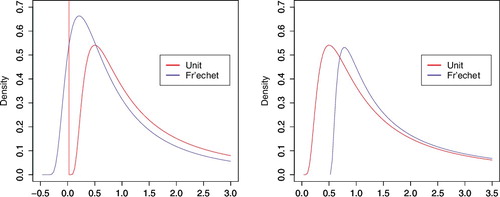
Our model in (Equation4(4) ) has two parts, the sparse M3 part and the hidden shock part. When β > 1, the hidden shock is dominated by the sparse M3 process in the upper tail region. The reverse is true when β < 1, while neither dominates with β = 1. See the asymptotic properties in Proposition 2.2 for more details. As for the location parameter, τ < 0 means the hidden shock has a reduced impact in the lower tail region compared to the sparse M3 process, and the reverse is the case for τ > 0. See for illustration using the density functions. β and τ therefore specify the role of Wt's as shock variables (or noise terms). An extreme value from Wt implies that Yt will be large while extreme value from Zlt implies Yt and Yt + l will likely both be large depending on the scaling constants (αl's) and random coefficients (Ults's).
It is unlikely, however, to observe data that will be on the same scale as the model in (Equation4(4) ); hence, we scale it with a parameter C. To further fit the shape of observable data more precisely, we add a shape parameter ψ. These parameterisations are reasonable. For example, the generalised extreme value distribution often applied to real data has scale and shape parameters. Our final model is, therefore, applicable to univariate financial time series data without any complex transformation of the data. Note that a data transformation can make interpretation of results difficult. Finally, we extend our model in (Equation4
(4) ) in the following manner:
(5) where C > 0 and ψ > 0 are scale and shape parameters, respectively.
Our models (Equation4(4) ) and (Equation5
(5) ) share the same structure of the models proposed in [26] where generalised method of moments (GMM) estimation procedure was utilised. In this work, we introduce an additional location parameter τ and develop a Bayesian inference approach which enables us to recover the strengths of random shock effects of Wt and to estimate the location parameter τ.
2.2. Model illustration
Two simulation examples of models (Equation4(4) ) and (Equation5
(5) ) are shown in . These two examples are from the same Vt and Wt latent processes. The parameters chosen here are close to the estimated parameters in our real data example in Section 4. The scaling parameters in α (L set to 3), which determined the dependence structure in Vt and hence in Yt and Xt, are set to (α1, α2, α3) = (0.5, 0.3, 0.2).
Figure 2. Simulation of models (Equation4(4) ) (left) and (Equation5
(5) ) (right) with size = 1000, (C, ψ, β, τ) = (0.001, 2, 1.5, −0.5) and α = (0.5, 0.3, 0.2). The horizontal lines are the 90th percentiles.
To highlight the roles of the two latent processes, using the same latent processes as the simulations in , we present more details in . On the left top-side we have the first 50 realisations. The dots are values of the latent process Vt when it equals Yt. On the top right, we have the 901st to the 950th realisations. Similarly, the dots are values of the latent process Wt when it equals Yt. As can be seen in the illustration, on the left, when the realisations are high and coming from Vt, they are high for extended periods. Although this will not always be the case depending on the values of scaling parameters in α and the random effects coming from the pertinent Ult's. On the right, it can be observed that extreme realisations are isolated when they come from Wt. Such a phenomenon is as a result of the independence structure of the Wt process. At the bottom, on the left of the figure, we present scatter plots of Yt vs. Vt from the first 50 realisations. On the right, we present scatter plots of Yt vs. Wt from the 901st to 950th realisations. Points on the diagonal are indications of when Yt equals the latent process, while points above the diagonal are from observations where Yt is greater than the latent process. Due to the specification of β = 1.5 for the Frećhet process Wt, the unit Frećhet Vt dominates in the right tail region, again, see . As a result, Yt = Vt more often, therefore, there are fewer values above the diagonal on the left than on the right. It should be noted that ψ changes the impact of extreme realisations in Yt significantly in Xt as can be seen in and .
Figure 3. Simulation of model (Equation4(4) ) with size = 1000, (β, τ) = (1.5, −0.5) and α = (0.5, 0.3, 0.2). Left side: First 50 realisations, t = 1 : 50. Right side: 901st to 950th realisations, t = 901: 950.
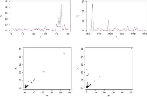
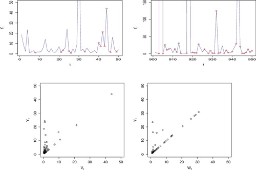
Figure 4. Simulation of models (Equation4(4) ) (left) and (Equation5
(5) ) (right) with size = 1000, (C, ψ, β, τ) = (0.001, 2, 0.7, 0.5) and α = (0.5, 0.3, 0.2). The horizontal lines are the 90th percentiles.
In and , we give more illustrations with a change from (β, τ) = (1.5, −0.5) to (β, τ) = (0.7, 0.5). Vt remains the same as in the previous simulation while Wt is different due to changes in shape and location parameters although the underlying unit Fréchet process remains the same. Comparing and , it can be seen that the values of Yt and Xt are significantly higher in . This observation is due to the values of the β and τ, but more importantly β causing a heavier right tail. Comparing and , our observations in is quite different from the observations in . In Figure , with identical time points as in , it can be seen in the illustration on the top-left that there are more isolated extreme realisations. This is due to the independent process Wt dominating in the right tail. On the right, it can still be observed that extreme realisations are isolated when they come from Wt. At the bottom, since Yt = Wt more often, there are more values above the diagonal on the left than on the right unlike in .
Figure 5. Simulation of model (Equation4(4) ) with size = 1000, (β, τ) = (0.7, 0.5) and α = (0.5, 0.3, 0.2). Left side: First 50 realisations, t = 1 : 50. Right side: 901st to 950th realisations, t = 901: 950. (Y30, Y904, Y918, Y943) = (110.2, 36749.2, 4545.1, 320.9) are out of the y-axis limits.
2.3. Theoretical properties
To look at the theoretical properties of our model, we first look at the distribution functions. The marginal distribution of our model (Equation4(4) ) is
for any yt > 0 and any index t, as shown in Section A.2.1.
The joint distribution takes the form:
for r ≥ 1 and yt > 0. U is the set of all relevant random variables on the interval [0, 1] and
(6) We note that the marginal does not depend on α, but the joint does. Hence, when β < 1, implying Wt is more dominant in the right tail, the estimation of α becomes harder than the estimation of α when β > 1, and the difficulty levels increase when β < 1 gets smaller. See Section A.2.2 for more detailed steps of the joint distribution.
To investigate the temporal dependence, we apply the asymptotic dependence index among other measures.
Definition 2.2:
Two random variables X1 and X2 with identical distribution function F are said to be asymptotically dependent (tail dependent) if,
(7) where
. If the limit of the above conditional probability is equal to 0, we say that X1 and X2 are asymptotically independent (tail independent).
The above definition of asymptotic dependence between two random variables is due to Sibuya (Citation1959) and an extension given by Ledford and Tawn (Citation2003), Zhang (Citation2005) and Zhang and Huang (Citation2006) is the lag-r asymptotic dependence index defined as follows.
Definition 2.3:
Let X1, X2, … be a stationary time series with distribution function F. If
while
where
, we say that the series is asymptotically dependent up to lag-r and λr is the lag-r asymptotic dependence index.
Next, we look at the asymptotic properties based on Definition 2.3 above. It should be noted that the asymptotic dependence index of model (Equation4(4) ) is identical to that of its counterpart, model (Equation5
(5) ), as the transformation is continuous.
Proposition 2.1:
The process (Equation4(4) ) is lag-L asymptotically dependent.
Proposition 2.2:
The process (Equation4(4) ) has asymptotic dependence index λl as
when β > 1;
0 when β < 1,
for 1 ≤ l ≤ L. When l > L, λl = 0.
The proofs of Propositions 2.1 and 2.2 are provided in Section A.2.4.
2.3.1. Stationarity and max-stablility
The next properties we look at are the stationarity of model (Equation4(4) ) and the max-stability of the sparse M3 part. This is necessary as we aim to model stationary time series data and we need max-stability following the earlier stated results of Smith and Weissman (Citation1996). From (Equation6
(6) ) it can be seen that the process is stationary as
for any r ≥ 1 and k ≥ 1. Also from (Equation6
(6) ), excluding the random shock part (or when β = 1 and τ = 0), it can be seen that the sparse M3 process is max-stable as Definition 2.1 is satisfied.
Result 2.1:
For any x > 0, the following holds for model (Equation5(5) ),
where
.
Result 2.1 can be used to study serial time dependence and we also apply it in our estimation approach for the αl's. The proof of Result 2.1 is in Section A.2.3.
Result 2.2:
A property of model (Equation5(5) ) is that when τ = 0, P(Xt ≤ C) = exp (−2).
This is from the following and setting τ = 0 and xt = C.
2.4. Estimation approach
There are previous works in the literature on the estimation of parameters of moving maxima processes. For example, Tang et al. (Citation2013) and Zhang and Zhu (Citation2016) used GMM due to Hansen (Citation1982). Bootstrap and empirical distribution techniques have also been proposed by Hall, Peng, and Yao (Citation2002), while Zhang and Smith (Citation2010) proposed the use of signature patterns among other methods. Here, we use Bayesian inference like Chamú-Morales (Citation2005) and Kunihama, Omori, and Zhang (Citation2011). In this section, we discuss relevant Markov chain Monte Carlo (MCMC) methods based on Robert and Casella (Citation2004) and Gelman, Carlin, Stern, and Rubin (Citation2003), and then proceed to our approach.
Notation
Let Θ[S] = (Θ1, Θ2,… , ΘS) be a d-dimensional chain and θs1: d = (θ1s, …, θsd) be a d-dimensional vector realisation of Θs for s = 1,… , S.
Our main focus here is on numerically evaluating integrals of the form
(8) without having to simulate samples directly from p mostly due to difficulty of doing so.
2.4.1. Hybrid MCMC
Since we have a multidimensional parameter space, we apply the Metropolis–Hasting algorithm from Metropolis et al. (Citation1953) and Hastings (Citation1970) in tandem with the Gibbs sampling technique from Geman and Geman (Citation1984) in what is called the hybrid MCMC shown below in Algorithm 1. Detailed discussion of our estimation approach is given in Appendix A.1.
Algorithm 1:
Hybrid MCMC
For k = 1, 2,… , d, from the most recent value (θs + 11, …, θk − 1s + 1, θsk, …, θds);
Step1. Generate
Step2. Set Θs + 1k as follow:
where
3. Simulation
The aim is to see how comparable estimated values are with true values. We have done extensive simulations with various parameter values. In this section, we present results for parameter values close to the estimated values from real market data in Section 4. We simulated a sample from model (Equation5(5) ) with a size of T = 5,000 and true parameter values as:
We set δ = 0.2 for estimation of parameters in α and the standard deviation for proposals chosen by trial-and-error as σκ = 0.02, ση = 0.03, kζ = 4, k′ζ = 0.01, kτ = 5 and k′τ = 0.005. For ρl(x*), we chose x* as the 90th percentile. The values were chosen so that we can have an acceptance rate of about 40% each time we attempted to change a transformation parameter and about 25% for α (two parameters) as recommended by Gelman, Roberts, and Gilks (Citation1996), Gelman et al. (Citation2003) for multidimensional problems. We ran the chain for 210,000 iterations and then discarded the first 10,000 as burn-in period. Due to autocorrelation, we thinned the remaining 200,000 by picking every 100th realisations and keeping them as samples drawn.
To monitor convergence, we apply the following diagnostic methods: (1) time plots to show the mixing of the chains; (2) density plots to show the estimated posterior distributions; (3) autocorrelation plots to show the autocorrelation function of the kept samples; and (4) acceptance rate from the original samples, which gives the ratio of the number of times that proposals are accepted to the number of iterations.
The MCMC outputs are presented in . They include time plots, estimated posterior distributions, and autocorrelation plots. Looking at the outputs and results in and , we can conclude that our estimation approach works well as we are able to successfully recover true parameter values with reasonable convergence measures.
Figure 6. Simulation Result 2.1: Graph of MCMC results for all parameters of model (Equation5(5) ), showing time plot, estimated posterior distribution and autocorrelation.
Table 1. Results of estimation for simulation example of model (Equation5(5) ).
In our tables, θp means 100× pth percentile and ‘Acc. Rate’ means acceptance rate.
To further test convergence property of our estimation approach, we use the test suggested by Gelman et al. (Citation2003). For M > 1 parallel draws, each of length S, we label each simulation drawn as {θsm, s = 1,… , S, m = 1,… , M}. Define
then the variance between (B) and within (W) sequences are compared. We can estimate the marginal posterior variance, Vθ of each parameter, defined as a weighted average of B and W in the following form,
Convergence can be monitored by checking the factor by which the scale of the current distribution for θ can be reduced when the chain is allowed to run indefinitely. The scale factor takes the form,
with
as the size of the chains goes to ∞. In Gelman et al. (Citation2003), it was stated that
is acceptable for most examples.
Following this approach, we tested convergence as follows. We ran M = 10 chains in parallel using the same simulated data and set-up as above. We let randomly chosen starting points be dispersed over a certain interval for each parameter. For C, we started between 0.0008 and 0.00012, and chose a starting point between 1 and 3 for β and ψ, while we started τ between −1 and 0. We started α1 and α2 between 0 and 0.5. We let each chain run for 210,000 iterations and discarded the first 10,000 as in the previous example. We, however, did not thin the draws. The value for each parameter is presented in . The results suggest that at 200,000 iterations, we attain convergence with each chain.
Table 2. Results of convergence test for simulation example of model (Equation5(5) ).
To check for sensitivity to prior, instead of using the unnormalised uniform priors on κ, η, ζ and τ (or logarithmic priors on κ, η, and ζ) as used previously, we use uniform priors on C, ψ and β over the range [0, ∞). This implies that the prior densities then take the form fκ∝exp (κ), fη∝exp (η), fζ∝exp (ζ) and for τ we leave it as before since it is not reparameterised. gives results from estimation on the same data using the newly chosen priors (uniform priors) versus results from the original priors (logarithmic priors). Although both choices of priors are locally uniform, they are different. The logarithmic prior places lower likelihood on larger values, hence penalising larger values, while the uniform prior does not. Based on results in and several other runs, we conclude that results from both are comparable.
Table 3. Results of sensitivity analysis for simulation example of model (Equation5(5) ).
Finally, as outputs in and are based on a single simulated sample, we further examined the performance of our proposed estimation approach for model (Equation5(5) ) on multiple samples. The results presented in are for 500 different simulated samples each with a size of T = 5,000 and true parameter values chosen as before.
Table 4. Results of estimation for 500 simulation examples, using median values of the parameters from each simualtion. [Int. C.P. means Interval Coverage Probability.]
To achieve this, we used parallel computing on a computer with multiple cores. For each sample, since the convergence was quickly reached, we let the chains run for 20,000 iterations and discarded the first 5000. We thinned the remaining 15,000 iterations by picking every 50th realisations and keeping the observed median values from each sample. Hence, we had a total of 500 estimated medians from each sample. Results of the medians are presented in . The results further suggest that our estimation approach works well for multiple samples.
For more tests of our estimation approach on model (Equation5(5) ), we further tested the performance with the case where β < 1. We simulated a sample from model (Equation5
(5) ) with a size of T = 5000 and true parameter values as:
For estimation, we set δ = 0.6 for α, σκ = 0.02, ση = 0.045, kζ = 10, k′ζ = 0.01, kτ = 20 and k′τ = 0.005. For ρl(x*), we chose x* as the 90th percentile. We ran the chains for 210,000 iterations and then discarded the first 10,000 as burn-in period. Due to autocorrelation, we thinned the remaining 200,000 by picking every 100th realisations and keeping them as samples drawn. Looking at the outputs and results in and , we can conclude that our estimation approach works well as we have been able to successfully recover true parameter values with reasonable convergence measures.
Table 5. Results of estimation for simulation example of model (Equation5(5) ).
4. Real data example
In this section, we carry out analysis of real data. We consider the univariate time series of intra-daily maxima of exchange returns from the US Dollar (USD) versus the Japanese Yen (JPY). The raw data contains 3-minute intra-daily prices for a time period between 31 December 2007, to 27 June 2013. The currencies traded six days weekly from Sunday to Friday. Hence, we have a total of 1720 trading days. There are four missing days that were filled by interpolation. The data was obtained from the University of Wisconsin-Madison Business School database. For each 3-minute period, we derived the negative log-returnFootnote2of the closing price versus the opening price, that is,
We further derived the daily (block) maxima of these values and used these as the values to which we applied model (Equation5
(5) ). By taking block maxima, the distribution of the observations is of the extreme value type. This means we can apply extreme value approaches to model tail dependence, clustering of extremes and to explain the volatility of the series. The time plot of the intra-daily maxima (which looks similar to the plot in ) is available in . We carried out augmented Dickey–Fuller and Phillips–Perron tests, both having p-values less than 0.01, suggesting that the series is stationary as it appears to be. For the lag value L, we chose L = 6 as there are six trading days each week. Hence, we can capture up to weekly lag effects.
Figure 7. Intra-daily maxima of the US Dollars vs. Japanese Yen 3-minute negative log-returns. The horizontal line is the 90th percentile.
We apply our estimation approach to estimate parameters that best fit the data. The values δ = 0.4, σκ = 0.035, ση = 0.05, kζ = 2, k′ζ = 0.01, kτ = 3 and k′τ = 0.005 were chosen so that we could have an acceptance rate of about 40% each time we attempted to change a transformation parameter and about 25% for α (5 parameters) as recommended by Gelman et al. (Citation1996) and Gelman et al. (Citation2003) for multidimensional problems. For ρl(x*), we chose x* as the 85th percentile. We ran the chain for 210,000 iterations and then discarded the first 10,000 as burn-in period. We thinned the remaining 200,000 by picking every 50th realisations and keeping them as samples drawn.
Our results are presented in . The MCMC outputs are presented in and . They include time plots, estimated posterior distributions and autocorrelation plots. Looking at the outputs in and , we can conclude that our estimation approach works well with reasonable convergence measures. From the posterior distributions in , the shape and scale parameters are significantly different from 1 as the credible intervals do not contain 1. Also, the location parameter τ is significantly different from 0, as the posterior mean of τ is −0.72, and the credible interval does not contain 0. From probabilistic properties of model Equation4(4) and the values of the estimated parameters, the random shock takes effect (Wt > Vt) about 30% of the time. To see how our estimated values fit the data, we use a quantile-quantile plot of real data versus simulated data using mean values and median values juxtaposed in . The plots suggest that our estimates fit the data well including in the right tail which is the main objective.
Figure 8. Real data analysis of USD vs JPY: Graph of MCMC results for transformation parameters of model (Equation5(5) ), showing time plot, estimated posterior distribution and autocorrelation.
Figure 9. Real data analysis of USD vs JPY: Graph of MCMC results for alpha parameters of model (Equation5(5) ), showing time plot, estimated posterior distribution and autocorrelation.
Figure 10. Quantile-quantile plots using estimated mean values on left and median values on right.
Table 6. Results of estimation for real data example of intra-daily maxima of 3-minute negative log-returns of USD vs. JPY.
5. Conclusion
We are able to develop a model for financial time series, starting with the M3 process. Our model (Equation5(5) ) can directly fit the data type without any transformations. The model also deals with random signature patterns and has sparsity in its loading matrix to better mirror real data. Given moving maxima models were often applied to filters obtained from some assumed processes, our proposed model is widely applicable.
Our estimation approach has been demonstrated to work. The use of adaptive jumping rules leads to the convergence of Markov chains. We conclude that adaptively scaling jumping kernels by the magnitude of current states gives stability to the samples drawn by the MCMC algorithm. Our work also shows that Bayesian inference can be useful in extreme value theory and estimation in parametric moving maxima processes.
For future work, we could consider similar models applicable to non-stationary series. This task can be achieved for example by having C to be time dependent, hence as Ct. Also, we could consider cases where the lag dependence structure in our sparse M3 process is different, and the random coefficients could take other distributions on the [0,1] interval. For example, based on Beta or Dirichlet distributions. Our model can also be extended to the multivariate case building on the multivariate maxima of moving maxima process (M4).
Acknowledgments
The authors thank the editor and referees for their valuable comments and suggestions. The work is partially supported by NSF-DMS-1505367 and NSF-CMMI-1536978.
Disclosure statement
No potential conflict of interest was reported by the authors.
Additional information
Funding
Notes on contributors
Timothy Idowu
Timothy Idowu earned a PhD in statistics from the University of Wisconsin-Madison. He currently works in quantitative finance in the Greater New York City area. Timothy was a doctoral student of the co-author Zhengjun Zhang.
Zhengjun Zhang
Zhengjun Zhang earned a PhD in statistics from the University of North Carolina at Chapel Hill. He is currently a full professor of statistics at the University of Wisconsin-Madison where he has taught statistics and supervised several doctoral students for over a decade.
Notes
1. The process Xt = max {αZt, (1 − α)Zt − 1} is called an MM(1) process where − ∞ < t < ∞, α ∈ (0, 1), Zt's are unit Fréchet random variables. If is considerably larger than
and
then we would have
.
2. A nice property of log-return is its time-additivity. Let , then
= rt, 1 + rt − 1, 1 + ⋅⋅⋅ + rt − k, 1.
3. 3The subcase where C > min (X) and τ ≥ 1 is not possible under the constraint.
References
- Box, G. E. P., & Jenkins, G. M. (1970). Time series analysis: Forecasting and control. San Francisco: Holden-Day.
- Chamú-Morales, F. (2005). Estimation of max-stable processes using Monte Carlo methods with applications to financial risk assessment ( PhD dissertation). Department of Statistics at the University of North Carolina, Chapel Hill, NC.
- Davis, R. A., & Resnick, S. I. (1989). Basic properties and prediction of Max-ARMA processes. Advances in Applied Probability, 21(4), 781–803.
- Deheuvels, P. (1983). Point processes and multivariate extreme values. Journal of Multivariate Analaysis, 13(2), 257–272.
- Fisher, R. A., & Tippett, L. H. C. (1928). Limiting forms of the frequency distribution of the largest and smallest member of a sample. Proceedings of Cambridge Philosophical Society, 24 (2), 180–190.
- Gelman, A., Roberts, G. O., & Gilks, W. R. (1996). Efficient metropolis jumping rules. Bayesian Statistics, 5, 599–607.
- Gelman, A., Carlin, J. B., Stern, H. S., & Rubin, D. B. (2003). Bayesian data analysis, 2e. Boca Raton, FL: CRC Press.
- Geman, S., & Geman, D. (1984). Stochastic relaxation, Gibbs distribution and the Bayesian restoration of images. IEEE Transactions on Pattern Analysis and Machine Intelligence, 6, 721–741.
- Gnedenko, B. V. (1943). Sur la distribution limite du terme maximum d'une serie aleatoire [On the limiting distribution of the maximum term in a random series]. Annals of Mathematics, 44(3), 423–453.
- Hall, P., Peng, L., & Yao, Q. (2002). Moving-maximum models for extrema of time series. Journal of Statistical Planning Inference, 103(1–2), 51–63.
- Hansen, L. P. (1982). Large sample properties of generalized method of moments estimator. Econometrica, 50(4), 1029–1054.
- Hastings, W. K. (1970). Monte carlo sampling methods using Markov chains and their application. Biometrika, 57(1), 97–109.
- Heffernan, J. E., Tawn, J. A., & Zhang Z,. (2007). Asymptotically (in)dependent multivariate maxima of moving maxima processes. Extremes, 10(1), 57–82.
- Kunihama, T., Omori, Y., & Zhang Z,. (2011). Efficient estimation and particle filter for max-stable processes. Journal of Time Series Analysis, 33(1), 61–80.
- Ledford, A. W., & Tawn, J. A. (2003). Diagnostics for dependence within time series extremes. Journal of the Royal Statistical Society: Series B (Statistical Methodology), 65(2), 521–543.
- McNeil, A. J., & Frey R,. (2000). Estimation of tail-related risk measures for heteroscedastic financial time series:An extreme value approach. Journal of Empirical Finance, 7(3-4), 271–300.
- Metropolis, N., Rosenbluth, A. W., Rosenbluth, M. N., Teller, A. H., & Teller E,. (1953). Equations of state calculations by fast computing machines. Journal of Chemical Physics, 21, 1087–1092.
- Pasarica, C., & Gelman, A. (2010). Adaptively scaling the metropolis algorithm using expected squared jumped distance. Statistica Sinica, 20, 343–364.
- Robert, C. P., & Casella, G. (2004). Monte carlo statistical methods, 2e. New York, NY: Spinger Text in Statistics.
- Sibuya, M. (1959). Bivariate extreme statistics. Annals of the Institute of Statistical Mathematics, 11(2), 195–210.
- Smith, R. L., & Weissman, I. (1996). Characterization and estimation of the multivariate extremal index. ( Tech. Report). Chapel Hill, NC: Department of Statistics at the University of North Carolina.
- Tang, R., Shao, J., & Zhang, Z. (2013). Sparse moving maxima models for tail dependence in multivariate financial time series. Journal of Statistical Planning and Inference, 143(5), 882–895.
- Zhang, Z. (2005). A new class of tail-dependent time series models and its applications in financial time series. Advances in Econometrics, 20(B), 323–358.
- Zhang, Z., & Huang, J. (2006). Extremal financial risk model and portfolio evaluation. Computational Statistics and Data Analysis, 51(4), 2313–2338.
- Zhang, Z., & Smith, R. L. (2010). On the estimation and application of max-stable processes. Journal of Statistical Planning and Inference, 140, 1135–1153.
- Zhang, Z., & Zhu, B. (2016). Copula structured M4 processes with application to high-frequency financial data. Journal of Econometrics, 194, 231–241.
Appendix
A.1. Estimation of parameters
Here, we give details of our estimation approach to the directly applicable model (Equation5(5) ). The goal is to draw samples from the joint posterior distribution using Algorithm 1.
The target distribution is the joint posterior distribution of parameters given observations x = (x1,… , xT). The full set of parameters is:
hence,
(A.1) Based on Bayes’ theorem, we have:
(A.2) where p(x|θ) is the likelihood of θ and p(θ) is its prior density with prior independence assumed among the parameters. We begin with some initial value θ1 that satisfies model constraints. In our examples, we use α1l = 1/L for l = 1,… , L, ψ1 = 1, β1 = 1, τ1 = 0 and C1 = exp (−2) × 100th percentile of the data based on Result 2.2. Numerically obtained maximum likelihood estimates can also be used as there are no analytic solutions.
We then iteratively draw S samples from θ|x with steps as follows and densities later defined:
for s = 1,… , S.
A.1.1. Sampling α
For α = (α1,… , αL) with dimension L (model is up to lag-L), we assume a uniform prior, that is, f(α)∝ constant. For each of the first L − 1 components of α, (α1,… , αL − 1), we generate proposals as follows. For state s + 1 with the current state as s, for each l = 1,… , L − 1, generate where q1( · |αsl) is the density function of the uniform distribution, Unif(max [αsl − δ, 0], min [αls + δ, 1]), with δ as a fixed disturbance. When we successfully simulate
such that
, we set
. We therefore have
which implies
For the likelihood, we use the tail dependence properties through the conditional probabilities of exceeding a given threshold. For a high threshold value x*, we introduce, ρl(x*) = ρl(x*; α, C, ψ, β, τ), nl(x*) and ωl(x*) defined as follows:
where I is the indicator function.
for each t = 1,… , T − l.
Calculation of ρl(x*) is based on Result 2.1. From many simulations, we find x* equal to the 85th, 90th and 95th percentiles appropriate.
With and treating the Ilt(x*)'s as Bernoulli random variables with the probability of success as ρl(x*), we have the likelihood for this step as:
(A.3)
(A.4) We therefore accept
with probability:
(A.5)
A.1.2. Sampling (log C, log ψ, log β, τ)
Set κ = log C, η = log ψ and ζ = log β. For all the steps, we use unnormalised uniform priors. The prior densities fκ, fη, fζ and fτ are therefore flat over the range of possible values for each parameter. For the likelihood we have:
(A.6) defined on the set
with C > 0, ψ > 0, β > 0 and
.
Given the constraint , we look at the range of values such that each parameter satisfies the constraint. We define min (X) as the smallest value in our observed data. We obtain the following ranges for parameters.
C > 0: Two cases, τ ≤ 0 and τ > 0.
Case 1: When τ ≤ 0;
Any C > 0 satisfies the constraint
Case 2: When τ > 0;
ψ > 0: Two cases. τ ≤ 0 and τ > 0.
Case 1: When τ ≤ 0;
Any ψ > 0 satisfies the constraint
Case 2: When τ > 0; Three subcasesFootnote3;
Subcase 1: C < min (X) and 0 < τ < 1;
Any ψ > 0 satisfies the constraint
Subcase 2: C < min (X) and τ ≥ 1;
Subcase 3: C > min (X);
β > 0:
Any β > 0 satisfies the constraint
We define as a truncated normal distribution with mean μ, variance σ2, lower bound a and upper bound b. For state s + 1 with the current state as s, simulate proposals for each parameter based on data and the current states of parameters as follows:
| (1) |
Accept | ||||
| (2) |
Case 1: exp (κs) < min (X) and τs ≥ 1
Case 2: exp (κs) > min (X)
Accept | ||||
| (3) |
Accept | ||||
| (4) |
Accept | ||||
Use of Adaptive Jumping Kernels
Adaptively scaling jumping kernels has been shown to improve convergence (see, for example, Pasarica & Gelman, Citation2010). In items 3 and 4 above, where we sample for ζ and τ, we use adaptive jumping kernels. The reason for this is the rapidly changing correlations between parameters in the model (for illustration, see ). The correlations can sometimes lead to rapid increase in the states of C and β while τ decreases rapidly (for illustration, see ). This is the case even under several re-parameterisations. However, by scaling the jumping kernels by the magnitude of the current state, we preempt such arbitrary fluctuations and even when they occur, and then the chains quickly move back to more probable states. The role of k′ζ and k′τ is to help the chain move away from states where ζ ≈ 0 (β ≈ 1) and τ ≈ 0, respectively. Without adaptively scaling jumping kernels, the chain could be stuck within those regions for long periods and even stay still in cases of equality.
Figure A1. Simulation result: Graph of MCMC results showing rapid fluctuation of parameters.
Figure A2. Simulation result: Graph of MCMC results showing scatter plot of parameters.
Figure A3. Unit Fréchet density (left) and Fréchet(β, 1, τ) density (right). Left: β = 1.5 and τ = −0.5. Right: β = 0.7 and τ = 0.5.
A.2. Proofs
A.2.1. Marginal distribution
A.2.2. Joint distribution
For r ≥ 1, xt > 0 and yt > 0 where t = 1,… , r.
where
(A.8)
(A.9)
A.2.3. Proof of Result 2.1
For 1 ≤ l ≤ L and y = (x/c)ψ.
(A.10)
(EquationA.10(A.10) ) equals
(A.11)
Therefore,
A.2.4. Proofs of Propositions 2.1 and 2.2
Using Equation (EquationA.11(A.11) ), for 1 ≤ l ≤ L and y = (x/c)ψ.
From Taylor's expansion and DCT, as y → ∞.
Case 1: β > 1,
Case 2: β = 1,
Case 3: β < 1,