The effects of additive outliers in INAR(1) process and robust estimation

ABSTRACT

In this paper, methods based on ranks and signs for estimating the parameters of the first-order integer-valued autoregressive model in the presence of additive outliers are proposed. In particular, we use the robust sample autocorrelations based on ranks and signs to obtain estimators for the parameters of the Poisson INAR(1) process. The effects of additive outliers on the estimates of parameters of integer-valued time series are examined. Some numerical results of the estimators are presented with a discussion of the obtained results. The proposed methods are applied to a dataset concerning the number of different IP addresses accessing the server of the pages of the Department of Statistics of the University of Würzburg. The results presented here give motivation to use the methodology in practical situations in which Poisson INAR(1) process contains additive outliers.

KEYWORDS:

• Additive outliers
• Poisson INAR(1) process
• robustness
• squared difference estimator

1. Introduction

Time series of count occur in many contexts, often as counts of events, objects or individuals in consecutive intervals or at consecutive points in time. Integer-valued time series data or count data arise naturally in many areas including finance (Brännäs, Hellströ, & Nordström, 2002), health science (Kachour & Yao, 2009), medicine (Franke & Seligmann, 1993), epidemiology (Zeger & Qaqish, 1988), economics (Freeland & McCabe, 2004) and others. In recent years, several models for the analysis of time series of count have been developed. For a review of models for analysis of time series of count, see Weiß (2008) and Scotto, Weiß, and Gouveia (2015).

In practical situation, it is quite common to have samples that have discrepant observations and they usually occur as a result of measurement errors, an influence of exogenous variables, a unexpected phenomenon among others situations. Such atypical observations are usually called as outliers (Fox, 1972). There are different class of outliers which have quite different impacts on an estimate (Denby & Martin, 1979). However, the most common types considered in the literature are: innovation outliers which produces an effect in all subsequent observations, additive outlier (AO) which affects only the level of the contaminated observation or replacement outliers, which have no effect on subsequent observations.

Several classes of robust estimators for ARMA models have been proposed (Martin & Yohai, 1985). Recently, the influence of outliers in time series has been the focus of much research (Fajardo, Reisen, & Cribari-Neto, 2009; Sarnaglia, Lévy-Leduc, & Reisen, 2010). For a review of robust estimation for ARMA models, see Martin and Yohai (1985). However, the study of robustness in time series of counts has not received much attention so far in the literature. Ispány, Barczy, Pap, Scotto, and Silva (2010,2011) consider conditional least squares (CLS) estimation of the parameters of the INAR(1) model contaminated, at known time periods, with innovational and additive outliers, respectively. The problem of detecting outliers in Poisson INAR(1) process has been investigated by Silva and Pereira (2015). Li, Lian, and Zhu (2016) considered the closed-form estimator for the INGARCH(1, 1) model and then robustify the closed-form estimator by replacing sample mean and autocorrelations by robust estimators of them, respectively. Silva and Silva (2018) considered the problem of detecting outliers, additive or innovational, single, multiple or in patches, in count time series modelled by Poisson INAR(1) process using wavelets. The motivation for studying integer-valued time series with atypical observations can be the fact that are quite common in many fields of application. Hence, it is an interesting research area in which to work. Furthermore, the robust procedures for estimating the parameters of the Poisson INAR(1) process has not yet been addressed in the literature. This paper aims to give a contribution in this direction. In this paper, robust estimators for the parameters of the Poisson INAR(1) process in the presence of additive outliers are obtained by replacing the classical autocovariance in the Yule–Walker (YW) equations by the robust autocovariance based on ranks and signs.

The rest of the paper unfolds as follows. In Section 2, the Poisson INAR(1) process is introduced, some of its basic properties are outlined and estimation methods for the model parameters is described. The impact of outliers on the correlation structure and estimation of the Poisson INAR(1) process is derivedin Section 3. In Section 4, we describe the robust procedures for estimating the autocorrelation function (ACF) and robust estimators for the parameters of the Poisson INAR(1) is proposed. Section 5 discusses some simulation results for the estimation methods. An application to real data is performed in Section 6. Some concluding remarks are addressed in Section 7.

2. Background: the Poisson INAR(1) process

In this section we provide a brief background of the Poisson INAR(1) process and the estimation of the unknown parameters.

2.1. The Poisson INAR(1) model

The INAR(1) model is based on the probabilistic operation of binomial thinning. Let the thinning operation , introduced by Steutel and Van Harn (1979) and let . If X is anynon-negative integer-valued random variable, is defined as , where are independent and identically distributed i.i.d random variables, independent of X, with , i.e. is an i.i.d. Bernoulli random sequence.

A discrete-time integer-valued stochastic process is said to be a first-order integer-valued autoregressive [INAR(1)] process if it satisfies the following equation (1) where , is a sequence of independent and identically distributed non-negative integer-valued random variables not depending on present and past values of . It is also assumed that the Bernoulli variables that define , that is, the Bernoulli variables from which are obtained, are independent of the Bernoulli variables from which other values of the series are calculated. Like for the first-order autoregressive process with normally distributed innovations, the conditional expectation of is linear in.

In this paper, it is assumed that is an i.i.d. sequence of Poisson distributed variables with mean and that, for all t, this sequence is mutually independent of all Bernoulli random variables that define . Also, we denote by , with , and that has the marginal distribution . Furthermore, the stationarity condition of the Poisson INAR(1) process is equivalent to that of the AR(1) process, i.e. if , then the integer-valued autoregressive process of order 1 is stationary. Many new results on it have been obtained in recent years to Poisson INAR(1) model. For example, Park and Oh (1997) studied the asymptotic properties of YW estimators, Hellström (2001) focused on the testing of a unit root, Freeland and McCabe (2005) obtained asymptotic properties of CLS estimators, Weiß (2011) proposed several asymptotic simultaneous confidence regions for the two parameters.

It is easy to verify that the ACF at lag k is given by (2) which obviously is restricted to be positive. Equation (2(2) ) shows that the autocorrelation function, , decays exponentially with lag k as happens in the classical AR(1) model.

2.2. Estimation of the unknown parameters

In practice, the true values of the model parameters α and μ are not known but have to be estimated from given time series data. There are several ways to estimate the parameters of Poisson INAR(1) process.

From a sample of a stationary process , the sample ACF is given by where denotes the sample mean. It is well-known that the estimators above are strongly consistent (Du & Li, 1991). The YW estimators of α and λ are based upon the sample ACF , using that , and the first moment of , which is . They are given by (3) Al-Osh and Alzaid (1987) and Brännäs (1994) suggested the use of the conditional maximum likelihood (CML) estimation to obtain the estimates. However, the CML estimators do not have closed-form expressions. The CLS estimation method was also considered in Freeland and McCabe (2005). Freeland and McCabe (2005) showed that the CLS estimators have the same asymptotic distribution as the YW estimators.

Weiß (2012) and Bourguignon and Vasconcellos (2015) suggested estimating the parameters of process using the squared difference (SD) estimator given by The alternative estimators discussed in the literature (YW, CML and CLS) feature perform much worse in terms of bias and mean square error than SD estimator (Bourguignon & Vasconcellos, 2015). For a good discussion of estimation in the Poisson INAR(1) process, the reader is referred to (Jung, Ronning, & Tremayne, 2005) and Bourguignon and Vasconcellos (2015).

3. The impact of AO in the Poisson INAR(1) process

The model contaminated by additive outliers is defined here as (4) where is the magnitude of the outliers (fixed and unknown parameter), 's are i.i.d. random variables, mutually independent of , with , with , i.e. is an i.i.d. Bernoulli random sequence with mean p and variance . The product is the expected number of outliers in the data. Note that from Equation (4(4) ) the outlier contribution in is random which is a reusable assumption since, in general, the occurrence of atypical observations in time series is not deterministic.

As previously discussed, outliers can affect the correlation structure of a time series and, consequently, the estimation of the model. The proof of Proposition 3.1 and Proposition 3.2 are given in the Appendix.

Proposition 3.1

Suppose that follows process (4(4) ) (5)

From this result, it can be seen that the AO increases the variance of which provokes a reduction of the ACF of the process. In addition, for all positive k, (6) Equation (6(6) ) shows that additive outliers introduce memory loss in the process . This leads to estimates with significant negative bias, as shown in Section 5.

Proposition 3.2

Let be generated from model (4(4) ) with one outlier with magnitude ω. It follows that:

1. The SD estimator for λ is given by

2. The SD estimator for α is given by

where is the sample mean of .

Corollary 3.1

Assume that is a stationary process with additive outliers as described in Equation  (4(4) ). Then,

1. .

4. .

Corollary 3.1 shows that additive outliers introduce significant positive bias in the SD estimator for λ parameter and significant negative bias in the SD estimator for α parameter, as shown in Section 5.

Propositions 3.1 and 3.2 show that the additive outliers can affect the statistical properties of the parameter estimates in Poisson INAR(1) process. In this context, it is necessary to use robust methods for estimating models of time series with outliers. This is the motivation of the next section.

3.1. An estimator for ω

In practice, the true value of the parameter ω is not known but have to be estimated from a given time series data. Let be generated from model (4) with outliers with magnitude ω. The estimator of ω is based on the sample mean of . Thus, the estimator of ω is given by (7) where and N is the number of outliers in the data, and . Thus, this estimator defined in (7(7) ) is the difference of mean of N observations that have outlier and the mean of T−N observations that have outlier.

Note that is an unbiased estimator for ω, i.e. . However, , then, we consider the version ‘corrected’ given by where represents the nearest integer.

Next, a small Monte Carlo simulation experiment will be conducted to evaluate the estimation of the ω in the Poisson INAR(1) process with additive outliers. The simulation was performed using the R programming language; see http://www.r-project.org. The number of Monte Carlo replications was 5000. The sample sizes considered are T=100,300,500. The contaminated data were generated from model (4) with p=0.01 and 0.05 for magnitudes and 10.

Table 1 presents the empirical mean and MSE of the estimates of the ω. From this table, notice that the biases and the mean square errors decrease as the size of the sample increases.

Table 1. Empirical means and MSEs (in parentheses) of the estimates of the parameter ω for and some values of T, p and ω.

		p=0.01			p=0.05
T	α
100	0.2	3.9532	5.4178	7.5030	4.8002	7.1566	10.078
		(0.7796)	(5.8058)	(16.355)	(1.3974)	(0.8614)	(0.9062)
	0.5	4.2424	5.3374	6.8268	5.1298	7.4324	10.169
		(0.9488)	(5.2450)	(16.908)	(2.3174)	(1.8616)	(2.7220)
	0.8	5.3116	5.9488	6.9822	6.2370	8.3636	11.131
		(2.9188)	(3.5472)	(14.516)	(6.6962)	(6.0228)	(9.561)
300	0.2	3.9672	5.6384	8.1600	4.7512	7.1734	10.077
		(0.4484)	(3.1436)	(7.5712)	(0.9491)	(0.2806)	(0.181)
	0.5	4.4028	5.5624	7.4160	5.2552	7.5744	10.2696
		(0.5672)	(3.0432)	(9.4096)	(2.0676)	(0.9552)	(0.8636)
	0.8	5.4436	6.2094	7.5316	6.4522	8.8528	11.877
		(2.7084)	(1.7822)	(8.9480)	(6.8710)	(5.4264)	(7.441)
500	0.2	3.9700	5.6536	8.2648	4.7340	7.1686	10.051
		(0.3476)	(2.5444)	(5.7412)	(0.8644)	(0.1970)	(0.0724)
	0.5	4.4902	5.5802	7.5264	5.3230	7.5878	10.2634
		(0.5538)	(2.6610)	(7.9940)	(2.1174)	(0.7746)	(0.5354)
	0.8	5.4942	6.2918	7.6646	6.4818	8.9434	12.013
		(2.6462)	(1.3142)	(7.4754)	(6.7494)	(5.0842)	(6.523)

4. Robust procedure to estimate parameters via nonparametric measures

The Kendall, Spearman, quadrant and Gaussian correlation coefficients are commonly used in nonparametric tests of independence between two variables (Hájek & Sidak, 1967). In this context it is assumed under the null hypothesis that the pairs are from a random sample bivariate, i.e. these pairs are i.i.d. This article is not of interest to test the independence between variables but estimate the degree of this dependence, this justifies the use of the coefficients in time series, i.e. here, the Kendall, Spearman, quadrant and Gaussian correlation coefficients, defined below, will be considered to estimate the ACF.

The estimator of the Kendall correlation coefficient (Kendall, 1938), based on the statistic , is where and The statistic is known as Kendall's sample rank correlation coefficient and appropriately assumes values between and 1, inclusive.

For a series generated by any process, the is used to estimate are defined as follows: where Now, let the pairs be a sample of size T of a random variable bivariate , and the associated pairs of ranks these observations. The Spearman rank correlation coefficient (Spearman, 1904) is defined by where . When there are ties values in the observations and/or , the coefficient Spearman correlation is calculated as follows: where in equation g denotes the number of tied X groups, is the size of tied X group i, l is the number of tied Y groups, and is the size of tied Y group j.

For a series generated by any process, the is used to estimate are defined as follows: where are the ranks of .

An estimation procedure can be endowed with robustness properties by using a rank statistics is the quadrant correlation coefficient (Blomqvist, 1950) that is the sample correlation coefficient between the signs of deviations from medians. To obtain a consistent version of the quadrant correlation at the normal model, we apply the transformation (Croux & Dehon, 2010).

The Gaussian rank correlation (Hájek & Sidak, 1967) is given (8) where the constant and is the quantile function of the standard normal distribution. For the treatment of ties observations see Hájek and Sidak (1967). For additional properties of the Gaussian rank correlation estimator, see Boudt, Cornelissen, and Croux (2012). Thus, for a series generated by any process, the is used to estimate using Equation (8(8) ) with being the ranks of .

Thanks to the use of ranks and signs, the Kendall, Spearman, quadrant and Gaussian correlations are resistant to small amounts of outliers in the data (Boudt et al., 2012). In this paper, robust estimators of the Poisson INAR(1) parameters are obtained by replacing the classical YW estimator in Equation (3(3) ) by the and estimators as follows

In next section, a Monte Carlo simulation will be conducted to evaluate the performance of the estimators discussed in this section.

5. Numerical results

In order to compare the performance of all the robust methodologies discussed previously, we performed a simulation study for different sample sizes and for different parameter values. All simulations were carried out using using the R programming language, which is freely distributed and available at see http://www.r-project.org. The data set was here generated from a Poisson INAR(1) process generated according to model (1(1) ) with being an i.i.d. Poisson sequence with mean . The contaminated data were generated from model (4(4) ) with p=0.02 for magnitudes and 7. The sample sizes considered were T=100,200,300 and the values of the α parameter in the simulation study were and 0.8. For each different situation the empirical mean and mean squared error (MSE) of the estimators were numerically estimated. The values of the MSE are given between parentheses. The number of Monte Carlo replications considered here was 5000. The results are presented in Tables 2 and 3.

Table 2. Empirical means and MSEs (in parentheses) of the estimates of the parameter α for p=0.02, , and some values of T and ω.

α	T	Estimator
0.2	100		0.1948 (0.0186)	0.0556 (0.0554)	−0.2747 (0.3553)
			0.1794 (0.0108)	0.1785 (0.0113)	0.1795 (0.0109)
			0.1718 (0.0105)	0.1780 (0.0105)	0.1923 (0.0097)
			0.1447 (0.0100)	0.1486 (0.0097)	0.1607 (0.0083)
			0.1105 (0.0122)	0.1192 (0.0111)	0.1264 (0.0099)
			0.1785 (0.0104)	0.1824 (0.0104)	0.1991 (0.0096)
	200		0.1981 (0.0092)	0.0555 (0.0377)	−0.2729 (0.2882)
			0.1902 (0.0053)	0.1902 (0.0057)	0.1901 (0.0055)
			0.1807 (0.0053)	0.1883 (0.0052)	0.2010 (0.0048)
			0.1523 (0.0058)	0.1572 (0.0054)	0.1678 (0.0044)
			0.1122 (0.0099)	0.1217 (0.0085)	0.1275 (0.0075)
			0.1885 (0.0051)	0.1934 (0.0052)	0.2092 (0.0049)
	300		0.1973 (0.0063)	0.0572 (0.0313)	−0.2722 (0.2659)
			0.1921 (0.0036)	0.1947 (0.0036)	0.1933 (0.0039)
			0.1818 (0.0036)	0.1920 (0.0033)	0.2014 (0.0033)
			0.1531 (0.0045)	0.1603 (0.0038)	0.1682 (0.0033)
			0.1114 (0.0093)	0.1223 (0.0075)	0.1259 (0.0070)
			0.1900 (0.0034)	0.1976 (0.0033)	0.2107 (0.0034)
0.8	100		0.7986 (0.0012)	0.7749 (0.0023)	0.7194 (0.0111)
			0.7556 (0.0067)	0.7558 (0.0068)	0.7566 (0.0065)
			0.7498 (0.0076)	0.7521 (0.0074)	0.7630 (0.0059)
			0.6288 (0.0337)	0.6287 (0.0337)	0.6424 (0.0288)
			0.5420 (0.0742)	0.5510 (0.0699)	0.5704 (0.0606)
			0.7514 (0.0068)	0.7524 (0.0067)	0.7586 (0.0058)
	200		0.7997 (0.0006)	0.7758 (0.0014)	0.7199 (0.0087)
			0.7767 (0.0028)	0.7785 (0.0027)	0.7768 (0.0027)
			0.7671 (0.0036)	0.7710 (0.0032)	0.7792 (0.0025)
			0.6445 (0.0263)	0.6462 (0.0258)	0.6570 (0.0223)
			0.5548 (0.0640)	0.5666 (0.0584)	0.5832 (0.0510)
			0.7726 (0.0028)	0.7750 (0.0027)	0.7780 (0.0024)
	300		0.7998 (0.0004)	0.7756 (0.0011)	0.7201 (0.0079)
			0.7854 (0.0016)	0.7852 (0.0016)	0.7846 (0.0017)
			0.7743 (0.0023)	0.7769 (0.0021)	0.7859 (0.0016)
			0.6511 (0.0236)	0.6513 (0.0235)	0.6633 (0.0199)
			0.5614 (0.0596)	0.5714 (0.0549)	0.5880 (0.0476)
			0.7813 (0.0017)	0.7821 (0.0016)	0.7866 (0.0014)

Table 3. Empirical means and MSEs (in parentheses) of the estimates of the parameter λ for p=0.02, , and some values of T and ω.

α	T	Estimator
0.2	100		1.0034 (0.0363)	1.2797 (0.1704)	1.8431 (1.1443)
			1.0228 (0.0248)	1.1096 (0.0444)	1.1679 (0.0696)
			1.0322 (0.0244)	1.1097 (0.0422)	1.1482 (0.0574)
			1.0666 (0.0252)	1.1502 (0.0497)	1.1941 (0.0707)
			1.1087 (0.0276)	1.1885 (0.0555)	1.2414 (0.0846)
			1.0239 (0.0241)	1.1040 (0.0414)	1.1388 (0.0547)
	200		1.0011 (0.0188)	1.2777 (0.1220)	1.8273 (0.8970)
			1.0110 (0.0128)	1.0935 (0.0247)	1.1530 (0.0437)
			1.0229 (0.0129)	1.0960 (0.0239)	1.1366 (0.0353)
			1.0586 (0.0145)	1.1384 (0.0324)	1.1843 (0.0495)
			1.1082 (0.0202)	1.1855 (0.0439)	1.2409 (0.0705)
			1.0132 (0.0125)	1.0891 (0.0229)	1.1250 (0.0324)
	300		1.0027 (0.0125)	1.2718 (0.1029)	1.8176 (0.8056)
			1.0091 (0.0083)	1.0849 (0.0176)	1.1463 (0.0348)
			1.0220 (0.0082)	1.0885 (0.0172)	1.1344 (0.0294)
			1.0580 (0.0103)	1.1315 (0.0257)	1.1821 (0.0437)
			1.1099 (0.0173)	1.1821 (0.0392)	1.2417 (0.0670)
			1.0117 (0.0080)	1.0809 (0.0161)	1.1213 (0.0259)
0.8	100		0.9986 (0.0306)	1.2101 (0.1037)	1.6161 (0.6162)
			1.2155 (0.1767)	1.3114 (0.2499)	1.3873 (0.3237)
			1.2450 (0.2019)	1.3321 (0.2732)	1.3499 (0.2906)
			1.8523 (0.8824)	2.0015 (1.1836)	2.0426 (1.2810)
			2.2830 (1.8985)	2.4166 (2.3018)	2.4452 (2.4063)
			1.2371 (0.1802)	1.3309 (0.2530)	1.3763 (0.2987)
	200		0.9977 (0.0157)	1.2064 (0.0722)	1.6012 (0.4768)
			1.1116 (0.0687)	1.1902 (0.1049)	1.2682 (0.1497)
			1.1598 (0.0873)	1.2308 (0.1269)	1.2542 (0.1384)
			1.7736 (0.6667)	1.9053 (0.9029)	1.9516 (0.9936)
			2.2203 (1.6051)	2.3324 (1.9136)	2.3683 (2.0245)
			1.1322 (0.0697)	1.2097 (0.1080)	1.2614 (0.1364)
	300		0.9986 (0.0102)	1.2116 (0.0647)	1.5970 (0.4326)
			1.0706 (0.0410)	1.1590 (0.0691)	1.2246 (0.1033)
			1.1259 (0.0573)	1.2040 (0.0892)	1.2168 (0.0959)
			1.7427 (0.5975)	1.8841 (0.8370)	1.9157 (0.8972)
			2.1903 (1.4988)	2.3145 (1.8243)	2.3416 (1.9013)
			1.0910 (0.0422)	1.1759 (0.0712)	1.2129 (0.0907)

Initially, the case where the series is not contaminated is analysed. It can be seen that the SD estimator presents much smaller biases (in absolute values) than the other estimators, for all cases. Tables 2 and 3 shows that additive outliers introduce significant positive bias in the SD estimator for λ parameter and significant negative bias in the SD estimator for α parameter.

For small sample sizes and , in general, both bias and MSE for the Spearman and Gaussian estimators are smaller than those for the SD, quadrant and YW methods. For , the bias for Gaussian estimators of α and λ is smaller than those for the SD, YW, quadrant and Spearman methods. Another result is related to the size of α. In general, for YW, Gaussian, qradrant and Spearman estimates of λ, increasing α, the bias and MSE also increase. This indicates that these four estimation methods of λ are sensitive to a process that is closer to the non-stationary boundary; that is, the model is more near a unit root Poisson INAR(1) process . The previous findings are confirmed by the box plots shown in Figure 1, which were obtained for sample size T=200 for some scenarios. Again, both biases and MSE for the Gaussian and Spearman estimators are smaller than those for the other methods.

Figure 1. Box plots from 5 000 simulated estimates of , p=0.02 and .

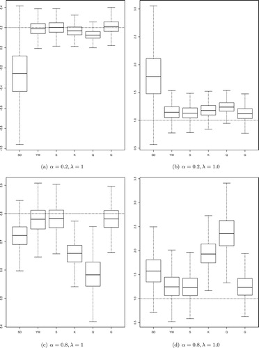
The empirical investigation here presented suggests that, in general, when there is no evidence of atypical observations, SD estimates give satisfactory results. The empirical study also provides evidence that special attention has to be paid when the data possibly exhibits atypical observations. The robust methodology showed that, in general, the estimates are essentially constant across different parameter values and outlier magnitudes.

6. Real data example: counts of IP addresses

In this section, we apply the methodology considered in Section 4 to a real data set. The data set consists of the number of different IP addresses accessing the server of the Department of Statistics of the University of Würzburg on 29 November 2005, between 10 am and 6 pm (241 observations). This series was previously studied by Weiß (2007), Zhu (2012a,b) and Silva and Pereira (2015). The required numerical evaluations for data analysis were here implemented using the R software.

The summary statistics are the following. All observations are lying between 0 and 8. The sample mean is 1.315, the sample median is 1 and the sample variance is 1.392. The lag-1 autocorrelation value is 0.219. Furthermore, We note that the ratio between the sample variance and the sample mean is 1.059, hence, the data seem to be equidispersed. We apply the test for overdispersion described by Schweer and Weiß (2014) with significance level at . The p-value for the test being 0.2870 leads to a not rejection of the null hypothesis of a Poisson INAR(1) process. Consequently, a Poisson marginal distribution would be appropriate. The series, sample autocorrelation and sample partial autocorrelation are displayed in Figure 2.

Figure 2. The time series plot, autocorrelation and partial ACFs for number of different IP addresses.

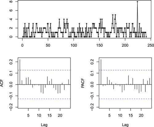
Analysing Figure 2, we conclude that a first-order autoregressive model may be appropriate for the given data series, because of the geometric decrease in the sample autocorrelations (as the lag increases) and the clear cut-off after lag 1 in the partial autocorrelations. Furthermore, thebehaviour of the series indicates that it may be mean stationary. According to Weiß (2007) and Silva and Pereira (2015), the observation at time t=224 is a possible occurrence of an outlier with . For this application, the estimates of α and λ were computed from the original data and from the modified data (without outlier). Therefore, we replaced the outlier by defining . As a consequence, the mean changes to 1.2863, the first-order autocorrelation to 0.2925, but an analysis of the resulting partial ACF and of the histogram showed that a Poisson INAR(1) model is still reasonable (Weiß, 2007).

In the Table 4, we present the estimates of the estimators discussed in this Sections 2 and 4 for the two series and the relative changes (RCs). The RCs are calculated from , where denotes the estimate of θ using the original data and denotes the estimate of θ using the modified data (without outlier). From Table 4, in both series, the robust methods present similar results. In contrast to the robust methods, the classics SD and YW estimators gives estimates that dramatically change from original data to without outlier data, showing that the observations is a possible outlier. Furthermore, note that the most important RCs are detected for the estimates of α, where the largest values are associated with SD and YW estimators.

Table 4. Estimates of the parameters and RCs for counts of IP data.

Estimator	Counts of IP data	Without outlier	RC	RC
	(0.1796, 1.0792)	(0.3424, 0.8458)	90.646	21.627
	(0.2195, 1.0267)	(0.2925, 0.9101)	33.257	11.357
	(0.2517, 0.9843)	(0.2680, 0.9416)	6.4760	4.2506
	(0.2109, 1.0381)	(0.2248, 0.9971)	6.5908	3.9495
	(0.1359, 1.1366)	(0.1362, 1.1110)	0.2208	2.2523
	(0.2480, 0.9892)	(0.2799, 0.9263)	12.863	6.3587

7. Conclusions

In this paper, some of the proposals for robust autocorrelation estimation are borrowed from the usual estimation of the parameters that index the Poisson INAR(1) model. Furthermore, this paper investigates the impact of additive outliers on estimating in the Poisson INAR(1) model. The number of different IP addresses data was analysed as an application of the methodology studied here. The results reveals that the robust methods (Spearman and Gaussian correlations) can be used as an alternative estimation for the parameters of the Poisson INAR(1) model contain additive outliers. In future research, the asymptotic properties of the robust estimators remain to be investigated.

Acknowledgments

We thank the associate editor and the reviewer for the constructive comments. The authors also would like to thank Professor Christian H. Weiß  for kindly providing the data set.

Disclosure statement

No potential conflict of interest was reported by the authors.

Appendix

Proof of Proposition 3.1

The proof of Proposition 3.1 is here omitted since it is a straightforward consequence of a result obtained by Fajardo et al. (2009).

Proof of Proposition 3.2

It is easy to see that Thus,

References

- Al-Osh, M. A., & Alzaid, A. A. (1987). First-order integer valued autoregressive (INAR(1)) process. Journal of Time Series Analysis, 8, 261–275. doi: 10.1111/j.1467-9892.1987.tb00438.x
- Blomqvist, N. (1950). On a measure of dependence between two random variables. The Annals of Mathematical Statistics, 21, 593–600. doi: 10.1214/aoms/1177729754
- Boudt, K., Cornelissen, J., & Croux, C. (2012). The Gaussian rank correlation estimator: Robustness properties. Statistics and Computing, 22, 471–483. doi: 10.1007/s11222-011-9237-0
- Bourguignon, M., & Vasconcellos, K. L. P. (2015). Improved estimation for Poisson INAR(1) models. Journal of Statistical Computation and Simulation, 85, 2425–2441. doi: 10.1080/00949655.2014.930862
- Brännäs, K. (1994). Estimation and testing in integer-valued AR(1) models. Umeå Economic Studies, 335. Retrieved from http://www.usbe.umu.se/digitalAssets/39/39107_ues335.pdf
- Brännäs, K., Hellströ, J., & Nordström, J. (2002). A new approach to modelling and forecasting monthly guest nights in hotels. International Journal Forecasting, 18, 19–30. doi: 10.1016/S0169-2070(01)00104-2
- Croux, C., & Dehon, C. (2010). Influence functions of the Spearman and Kendall correlation measures. Statistical Methods and Applications, 19, 497–515. doi: 10.1007/s10260-010-0142-z
- Denby, L., & Martin, R. D. (1979). Robust estimation of the first order autoregressive parameter. Journal of the American Statistical Association, 74, 140–146. doi: 10.1080/01621459.1979.10481630
- Du, J., & Li, Y. (1991). The integer valued autoregressive (INAR(p)) model. Journal of Time Series Analysis, 12, 129–142. doi: 10.1111/j.1467-9892.1991.tb00073.x
- Fajardo, F., Reisen, V. A., & Cribari-Neto, F. (2009). Robust estimation in long-memory processes under additive outliers. Journal of Statistical Planning Inference, 139, 2511–2525. doi: 10.1016/j.jspi.2008.12.014
- Fox, A. J. (1972). Outliers in time series. Journal of the Royal Statistical Society B, 34, 350–363.
- Franke, J., & Seligmann, T. (1993). Conditional maximum-likelihood estimates for INAR(1) processes and their application to modelling epileptic seizure counts. In T. Subba Rao (Ed.), Developments in time series (pp. 310–330). London: Chapman & Hall.
- Freeland, R. K., & McCabe, B. P. M. (2004). Analysis of low count time series data by Poisson autoregression. Journal of Time Series Analysis, 25, 701–722. doi: 10.1111/j.1467-9892.2004.01885.x
- Freeland, R. K., & McCabe, B. P. M. (2005). Asymptotic properties of CLS estimators in the Poisson AR(1) model. Statistics and Probability Letters, 73, 147–153. doi: 10.1016/j.spl.2005.03.006
- Hájek, J., & Sidak, Z. (1967). Theory of rank tests. New York, NY: Academic Press.
- Hellström, J. (2001). Unit root testing in integer-valued AR(1) models. Economics Letters, 70, 9–14. doi: 10.1016/S0165-1765(00)00344-X
- Ispány, M., Barczy, M., Pap, G., Scotto, M., & Silva, M. E. (2010). Innovational outliers in INAR(1) models. Communications in Statistics – Theory and Methods, 39, 3343–3362. doi: 10.1080/03610920903259831
- Ispány, M., Barczy, M., Pap, G., Scotto, M., & Silva, M. E. (2011). Additive outliers in INAR(1) models. Statistical Papers, 53, 935–949.
- Jung, R. C., Ronning, G., & Tremayne, A. R. (2005). Estimation in conditional first order autoregression with discrete support. Statistical Papers, 46, 195–224. doi: 10.1007/BF02762968
- Kachour, M., & Yao, J. F. (2009). First-order rounded integer-valued autoregressive (RINAR(1)) process. Journal of Time Series Analysis, 30, 417–448. doi: 10.1111/j.1467-9892.2009.00620.x
- Kendall, M. G. (1938). A new measure of rank correlation. Biometrika, 30, 81–93. doi: 10.1093/biomet/30.1-2.81
- Li, Q., Lian, H., & Zhu, F. (2016). Robust closed-form estimators for the integer-valued GARCH(1,1) model. Computational Statistics and Data Analysis, 101, 209–225. doi: 10.1016/j.csda.2016.03.006
- Martin, R. D., & Yohai, V. J. (1985). Robustness in time series and estimating ARMA models. In E. J. Hannan et al. (Eds.), Handbook of statistics (Vol. 5, p. 119–155). Science Publishers B.V. New York.
- Park, Y., & Oh, C. W. (1997). Some asymptotic properties in INAR(1) processes with Poisson marginals. Statistical Papers, 38, 287–302. doi: 10.1007/BF02925270
- Sarnaglia, A. J. Q., Lévy-Leduc, V. A., & Reisen, C. (2010). Robust estimation of periodic autoregressive processes in the presence of additive outliers. Journal of Multivariate Analysis, 101, 2168–2183. doi: 10.1016/j.jmva.2010.05.006
- Schweer, S., & Weiß, C. (2014). Compound Poisson INAR(1) processes: Stochastic properties and testing for overdispersion. Computational Statistics and Data Analysis, 77, 267–284. doi: 10.1016/j.csda.2014.03.005
- Scotto, M. G., Weiß, C. H., & Gouveia, S. (2015). Thinning-based models in the analysis of integer-valued time series: A review. Statistical Modelling, 15, 590–618. doi: 10.1177/1471082X15584701
- Silva, M. E., & Pereira, I. (2015). Detection of additive outliers in Poisson INAR(1) time series. In Mathematics of Energy and Climate Change, 2, 377–388. doi: 10.1007/978-3-319-16121-1_19
- Silva, I, & Silva, M. E. (2018). Wavelet-based detection of outliers in Poisson INAR (1) time series. In Recent studies on risk analysis and statistical modeling. New York. Springer, 2018.
- Spearman, C. (1904). General intelligence objectively determined and measured. The American Journal of Psychology, 15, 201–293. doi: 10.2307/1412107
- Steutel, F. W., & Van Harn, K. (1979). Discrete analogues of self-decomposability and stability. The Annals of Probability, 7, 893–899. doi: 10.1214/aop/1176994950
- Weiß, C. H. (2007). Controlling correlated processes of Poisson counts. Quality and Reliability Engineering International, 23, 741–754. doi: 10.1002/qre.875
- Weiß, C. H. (2008). Thinning operations for modelling time series of counts - a survey. Advances in Statistical Analysis, 92, 319–341. doi: 10.1007/s10182-008-0072-3
- Weiß, C. H. (2011). Simultaneous confidence regions for the parameters of a Poisson INAR(1) model. Statistical Methodology, 8, 517–527. doi: 10.1016/j.stamet.2011.07.003
- Weiß, C. H. (2012). Process capability analysis for serially dependent processes of Poisson counts. Journal of Statistical Computation and Simulation, 82, 383–404. doi: 10.1080/00949655.2010.533178
- Zeger, S. L., & Qaqish, B. (1988). Markov regression models for time series: a quasi-likelihood approach. Biometrics, 44, 1019–1031. doi: 10.2307/2531732
- Zhu, F. (2012a). Modeling overdispersed or underdispersed count data with generalized Poisson integer-valued GARCH models. Journal of Mathematical Analysis and Applications, 389, 58–71. doi: 10.1016/j.jmaa.2011.11.042
- Zhu, F. (2012b). Modeling time series of counts with COM-Poisson INGARCH models. Mathematical and Computer Modelling, 56, 191–203. doi: 10.1016/j.mcm.2011.11.069