Topic model for graph mining based on hierarchical Dirichlet process

Abstract

In this paper, a nonparametric Bayesian graph topic model (GTM) based on hierarchical Dirichlet process (HDP) is proposed. The HDP makes the number of topics selected flexibly, which breaks the limitation that the number of topics need to be given in advance. Moreover, the GTM releases the assumption of ‘bag of words’ and considers the graph structure of the text. The combination of HDP and GTM takes advantage of both which is named as HDP–GTM. The variational inference algorithm is used for the posterior inference and the convergence of the algorithm is analysed. We apply the proposed model in text categorisation, comparing to three related topic models, latent Dirichlet allocation (LDA), GTM and HDP.

Keywords:

• Graph topic model
• hierarchical Dirichlet process
• variational inference
• text classification

1. Introduction

We are entering the era of big data. It becomes more difficult for people to find valuable information from the explosion of document archives. New techniques or tools need to be used to deal with automatically organising, searching and understanding large collections. Topic modelling provides a convenient way to analyse big unstructured text (Miner et al., 2012). A topic model is a kind of a probabilistic generative model that has been used widely in the field of computer science text mining and information retrieval in recent years (Gupta & Lehal, 2009).

The origin of the probabilistic topic model is latent semantic indexing (LSI) (Deerwester, 1990); it has been the basis for the development of the topic model. Based on LSI, probabilistic latent semantic analysis (PLSA) (Hofmann, 1999) was proposed by Hofmann and is probabilistic topic modelling. Latent Dirichlet allocation (LDA) proposed by Blei, Ng, and Jordan (2003) is a method using probabilistic generative models. The basic assumption of LDA is ‘bag of word’ which means the order of the words can be neglected. Recently, there are many methods using probabilistic topic models that are based on LDA via combination with particular tasks and relaxing the assumption of LDA (Blei, 2012). In many text analysis settings, a document is composed of the words which serve as nodes, and the relations between words serve as edges (Valle, 2011). The relations may be co-occurrence relations, association relations or other semantic relations. Then, the text is expressed as graph structure data. The research of graph structure data belongs to the field of graph mining. The idea of graph mining to the topic model can improve the accuracy of classification or clustering of text graph structure data compared with text mining which only considers nodes but ignores the relationship between them. In addition, many practical tasks can all benefit from this kind of graph mining such as products, services and website retrieval. Although topic models have proved to be very successful in discovering latent topics, the standard topic models cannot be directly applied to graph-structured data because of the ‘bag-of-word’ assumption. Xuan, Lu, Zhang, and Luo (2015) proposed a method using topic model for graph mining (GTM) which assumes that there is an edge between two nodes in a graph, these two nodes tend to talk similar content.

In LDA, the topics are fixed for the whole corpus, and the number of topics is assumed to be known in advance. However, it is usually hard to make such a decision without a deep knowledge of the data set. Recent advances in Bayesian nonparametric modelling, specifically hierarchical Dirichlet process (HDP) (Gershman & Blei, 2012; Teh, Jordan, Beal, & Blei, 2006), has lead to ‘infinite’ topic models. The number of topics does not need to be specified and is determined by collection during the posterior inference and furthermore, new documents can exhibit previously unseen topics. This paper proposes a method using graph topic model based on hierarchical Dirichlet process (HDP-GTM). HDP-GTM realises the flexible selection of topic numbers by the property of HDP, breaking through the limitation that classical topic models in advance. At the same time, this method breaks through the limitation of the assumption ‘bag of word’ and takes the graph structure of the text into account which can make full use of data information, thus the text classification accuracy can be significantly improved.

Exactly computing posterior distributions for the HDP-GTM is very intractable. We propose a variational inference algorithm for the HDP-GTM. Variational inference (VI) is a method from machine learning for approximating probability densities (Blei, Kucukelbir, & McAuliffe, 2017; Jordan, Ghahramani, Jaakkola, & Saul, 1999; Wainwright & Jordan, 2008). Variational inference is widely used to approximate posterior densities for Bayesian models, an alternative strategy to Markov chain Monte Carlo (MCMC) sampling. Compared to MCMC, variational inference tends to be faster and easier to scale to large datasets. It has been applied to problems such as large-scale document analysis, computational neuroscience and computer vision. But variational inference has been studied less rigorously than MCMC, and its statistical properties are less well understood. In this paper, we apply a variational inference algorithm for calculating the posterior distribution and investigate its convergence property.

The structure of this paper is as follows. We provide a brief introduction of the related models LDA, HDP and GTM in Section 2. Then, in Section 3, we propose HDP–GTM based on HDP and GTM. The posterior inference is derived by the variational inference procedure and the convergence of variational inference algorithm is verified in Section 4. Finally, in Section 5, experiments are conducted to compare the performance of the HDP–GTM with LDA, HDP and GTM on the Reuter dataset and the 20-newsgroup dataset. Section 6 concludes the paper with some concluding remarks.

2. Related work

This section will provide more details about LDA, GTM, and HDP respectively.

2.1. Latent Dirichlet allocation

First, we review the underlying statistical assumptions of the LDA. The LDA is a method using three-level hierarchical Bayesian model which includes three levels of documents, topics and words. LDA adds a priori distribution of document-topic level and topic-word level. LDA assumes that the probability of document-topic is $p\left(z|d\right)$ extracted from Dirichlet distribution $\mathrm{Dir}\left(\alpha \right)$ and the probability of topic-word is $p\left(w|z\right)$ extracted multinomial distribution respectively. The Dirichlet distribution and multinomial distribution are conjugate prior distributions, which can simplify the calculation of the posterior distribution. The graphical representation of LDA is shown in Figure 1 and each document is assumed drawn from the following generative process:

1. Draw the topic proportion ${\theta }_d\stackrel{\mathrm{i}.\mathrm{i}.\mathrm{d}.}{\sim }\mathrm{Dir}\left(\alpha \right)$ for each document;

2. Draw ${\phi }_k\stackrel{\mathrm{i}.\mathrm{i}.\mathrm{d}.}{\sim }\mathrm{Dir}\left(\beta \right)$ for each topic;

3. For each word n in the document d:

   1. Draw topic assignment $z_{dn}\stackrel{\mathrm{i}.\mathrm{i}.\mathrm{d}.}{\sim }\mathrm{Multi}\left({\theta }_d\right)$;

   2. Draw $w_{dn}|\{\phi {\}}_{k=1}^{\mathrm{\infty }},z_{dn}\sim \mathrm{Multi}({\phi }_{z_{dn}})$ for each word.

Figure 1. Graphical model representation of LDA.

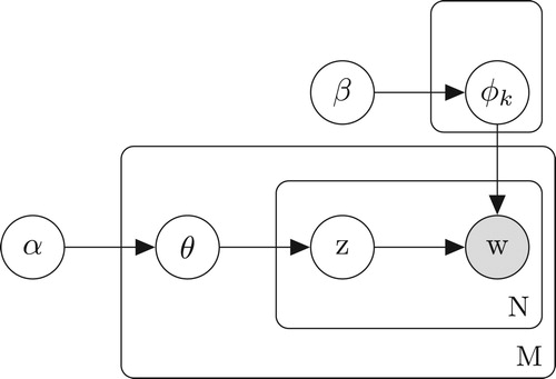
As the figure makes clear, there are three levels to the LDA representation. The parameters α and β are corpus-level parameters, assumed to be sampled once in the process of generating a corpus. The variables ${\theta }_d$ are document-level variables, sampled once per document. Finally, the variables $z_{dn}$ and $w_{dn}$ are word-level variables and are sampled once for each word in each document. It is difficult to compute the posterior distribution directly, two commonly used methods are variational EM algorithm which aims at looking to the approximate Bayesian estimate of $p(w|\alpha ,\beta )$ (Blei et al. 2003) and the other method is Gibbs sampling (Griffiths & Steyvers, 2004).

LDA considers the prior distribution of parameters, and the topic distribution is no longer fixed, but obtained by sampling. However, LDA is based on the ‘bag of words’ assumption, regardless of the order of words, and regardless of the correlation between words. In this way, some important information in the text will be omitted, resulting in information loss.

2.2. Graph topic model

The traditional topic models are based on the assumption of ‘bag of words’, that is, words in text are independent and exchangeable (Aldous, 1985). Exchangeability means that we don't consider the order in which the locations of words appear in the text, nor do we consider the association between words. Although topic model has been popular in the field of text mining and information retrieval, the research on topic mining of graph structure text data is insufficient. Xuan, Lu, Zhang, and Luo (2015) proposed a method using probabilistic topic model based on graph structure data which was inspired by graph structure text data.

GTM is an extension of LDA which the graph structure of text data is considered. Although the traditional topic model is considered very successful, traditional topic models cannot be directly applied to graph structure text data because of the ‘bag of word’ assumption of the topic model. In the graph topic model, $w_{dn}$ indicates a node in the document d and $e_{w_{di},w_{dj}}$in the document d indicates the edge between the node $w_{di}$ and the node $w_{dj}$ corresponding to the relationship between words. Applying GTM to text data requires adding an edge parameter e in LDA model. Assuming that two nodes describe similar topics, it is considered that there is an edge between these two nodes. The edge is a parameter that describes the topic similarity of the nodes, therefore, $e_{w_{di},w_{dj}}$ can be generated by the topic distribution of node $w_{di}$ and node $w_{dj}$.

The graphical representation of GTM is shown in Figure 2 and the corresponding generative process is as follows.

1. Draw topic proportion ${\theta }_d\stackrel{\mathrm{i}.\mathrm{i}.\mathrm{d}.}{\sim }\mathrm{Dir}\left(\alpha \right)$ for each document

2. Draw ${\phi }_k\stackrel{\mathrm{i}.\mathrm{i}.\mathrm{d}.}{\sim }\mathrm{Dir}\left(\beta \right)$ for each topic

3. Draw topic assignment $z_{dn}\stackrel{\mathrm{i}.\mathrm{i}.\mathrm{d}.}{\sim }\mathrm{Multi}\left({\theta }_d\right)$

4. Draw $w_{dn}|\{\phi {\}}_{k=1}^{\mathrm{\infty }},z_{dn}\sim \mathrm{Multi}({\phi }_{z_{dn}})$ for each word node

5. For all edges in a graph: draw $e_{w_{di},w_{dj}}\sim \mathrm{Bernoulli}\left(p_{w_{di},w_{dj}}\right)$ for each edge, where (1) $p_{w_{di},w_{dj}}(e_{w_{di},w_{dj}}=1)={\phi }_{z_{di}}\cdot {\phi }_{z_{dj}}$(1)

$e_{w_{di},w_{dj}}$ is the edge between word $w_{di}$ and word $w_{dj}$ which is extracted from Bernoulli distribution, and $p_{w_{di},w_{dj}}$ is the parameter of Bernoulli distribution.

Figure 2. Graphical model representation of GTM.

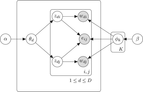
From Figure 2, $e_{w_{di},w_{dj}}$ is generated from $\{z_{di},z_{dj},\mathrm{\Phi }\}$, so it means that the probability of the existence of an edge between two nodes is determined by the similarity of their topic distributions. This similarity is measured by vector inner product of ${\phi }_{z_{di}}$ and ${\phi }_{z_{dj}}$, where ${\phi }_{z_{di}}$ is node distribution of topic $z_{di}$, as shown in Equation (1(1) $p_{w_{di},w_{dj}}(e_{w_{di},w_{dj}}=1)={\phi }_{z_{di}}\cdot {\phi }_{z_{dj}}$(1) ). The more similar topics of two keywords are, the more likely there is an edge between these two nodes. Different from the ‘bag of words’ assumption of the traditional topic model, Bernoulli distribution is used to model the relationship between two keywords, and the similarity between two theme distributions of two keywords is parameterised in GTM. By considering the relationship between key words in the document, GTM is verified better than LDA through the experimental results of text classification GTM is derived from LDA, and both of these models belong to Bayesian models. Similar to LDA, the deficiency of GTM model lies in that the number of topics needs to be given in advance, it is difficult to make such a decision without a deep knowledge of the dataset. HDP is a Bayesian nonparametric method for modelling topic model, the number of topics does not need to be specified in advance and is determined by collection during posterior inference.

2.3. Hierarchical Dirichlet process

HDP is useful in problems in which there are multiple groups of data (Teh et al., 2006; Wang et al. 2011). The HDP is a hierarchical extension to Dirichlet process (DP) (Blackwell & MacQueen, 1973; Ferguson, 1973). The hierarchical structure provides an elegant way of sharing parameters. Mathematically, (2) $\begin{array}{rl}{G}_0& \sim \mathrm{DP}(\gamma ,H),\\ G_d& \sim \mathrm{DP}({\alpha }_0,G_0),\mathrm{for}\mathrm{each}\mathrm{document}\mathrm{d},\end{array}$(2) where H is the base probability measure, γ and ${\alpha }_0$ are concentration parameters. The distribution $G_0$ varies around H by an amount controlled by γ and the distribution $G_d$ in group d varies around $G_0$ by an amount controlled by ${\alpha }_0$.

The HDP can be seen as adding another level of smoothing on top of DP mixture models. For each d, let ${\theta }_{d1},{\theta }_{d2},\dots$ be iid random variables distributed as $G_d$. Each ${\theta }_{dn}$ is a factor corresponding to a single observation $w_{dn}$. The likelihood is given by (3) $\begin{array}{rl}{\theta }_{dn}|G_d& \sim G_d,\\ w_{dn}|{\theta }_{dn}& \sim \mathrm{Multi}\left({\theta }_{dn}\right).\end{array}$(3) Sticking-breaking priors are rich and important class of random measures in Bayesian Nonparametric which origins in Ferguson (1973) and Sethuraman (1994) proposed infinite mixture representation of the Dirichlet process. HDP can be constructed by stick-breaking method which was shown in Teh, Jordan, Beal and Blei (2006). We describe an alternative stick-breaking construction for the HDP proposed by Wang, Paisley and Blei (2011). For the corpus-level DP draw, this representation is (4) $\begin{array}{rl}& {\beta }_k^{\mathrm{\prime }}\sim \mathrm{Beta}(1,\gamma ),\\ & {\beta }_k={\beta }_k^{\mathrm{\prime }}\prod _{\ell =1}^{k-1}(1-{\beta }_{\ell }^{\mathrm{\prime }}),\\ & {\phi }_k\stackrel{\mathrm{i}.\mathrm{i}.\mathrm{d}.}{\sim }H,\\ & G_0=\sum _{k=1}^{\mathrm{\infty }}{\beta }_k{\delta }_{{\phi }_k}.\end{array}$(4) Thus $G_0$ is discrete and has support at the atoms $\mathit{\phi }=({\phi }_k{)}_{k=1}^{\mathrm{\infty }}$ with weights $\mathit{\beta }=({\beta }_k{)}_{k=1}^{\mathrm{\infty }}$. The distribution for $\mathit{\beta }$ is written as $\mathit{\beta }\sim \mathrm{GEM}\left(\gamma \right)$ which stands for Griffiths, Engen, and McCloskey (Pitman 2002). The construction of each document-level $G_j$ by Sethuraman's stick-breaking construction is (5) $\begin{array}{rl}& {\pi }_{dt}^{\mathrm{\prime }}\sim \mathrm{Beta}(1,\alpha ),\\ & {\pi }_{dt}={\pi }_{dt}^{\mathrm{\prime }}\prod _{\ell =1}^{t-1}(1-{\pi }_{d\ell }^{\mathrm{\prime }}),\\ & {\pi }_{dt}\stackrel{\mathrm{i}.\mathrm{i}.\mathrm{d}.}{\sim }{G}_0,\\ & G_d=\sum _{t=1}^{\mathrm{\infty }}{\pi }_{dt}{\delta }_{{\psi }_t}.\end{array}$(5) Notice that each document-level atom ${\psi }_{dt}$ maps to a corpus-level atom ${\phi }_k$ in $G_0$ according to the distribution defined by $G_0$. The distribution for ${\mathit{\pi }}_d$ is also written as ${\mathit{\pi }}_d\sim \mathrm{GEM}\left(\alpha \right)$. Let ${\mathit{c}}_d=(c_{dt}{)}_{t=1}^{\mathrm{\infty }}$ be a series of indicator variables which are drawn i.i.d., (6) $c_{dt}\stackrel{\mathrm{i}.\mathrm{i}.\mathrm{d}.}{\sim }\mathrm{Mult}\left(\mathit{\beta }\right),$(6) where $\mathit{\beta }\sim \mathrm{GEM}\left(\gamma \right)$. Then let (7) ${\psi }_{dt}={\phi }_{c_{dt}}.$(7) Thus we do not need to explicitly represent the document atoms ${\mathit{\psi }}_j$. The property that multiple document-level atoms ${\psi }_{dt}$ can map to the same corpus-level atom ${\phi }_k$ in this representation which is similar in spirit to the Chinese restaurant franchise (CRF) (Teh et al., 2006), where each restaurant can have multiple tables serving the same dish ${\phi }_k$. In the CRF representation, a hierarchical Chinese restaurant process allocates dishes to tables. Here, we use a series of random indicator variables ${\mathbf{c}}_d$ to represent this structure. Given the representation in Sethuraman's stick-breaking construction, the generative process for the observed words in the dth document is as follows: (8) $\begin{array}{rl}& z_{dn}\stackrel{\mathrm{i}.\mathrm{i}.\mathrm{d}.}{\sim }\mathrm{Mult}\left({\mathit{\pi }}_d\right),\\ & {\theta }_{dn}={\psi }_{d{z}_{dn}}={\phi }_{c_{d{z}_{dn}}},\\ & w_{dn}\stackrel{\mathrm{i}.\mathrm{i}.\mathrm{d}.}{\sim }\mathrm{Mult}\left({\theta }_{dn}\right).\end{array}$(8) The indicator $z_{dn}$ selects topic parameter ${\psi }_{dt}$, which maps to one topic ${\phi }_k$ through the indicators $c_{dt}$. 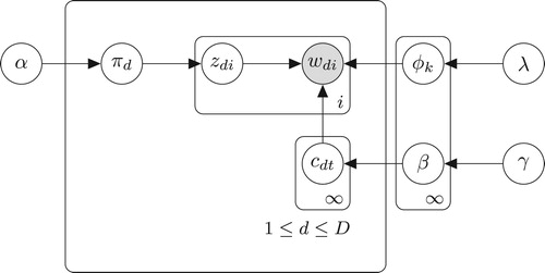The graphical representation of GTM is shown in Figure 3 and HDP topic model is described below:

1. Draw $\mathit{\beta }\sim \mathrm{GEM}\left(\gamma \right)$ and ${\mathit{\pi }}_d\sim \mathrm{GEM}\left(\alpha \right)$

2. Draw ${\phi }_k\stackrel{\mathrm{i}.\mathrm{i}.\mathrm{d}.}{\sim }\mathrm{Dir}\left({\lambda }_k\right)$

3. For each word $w_{dn}$ in the document d where $n\in \{1,2,\dots ,N_d\}$ and $t\in \{1,2\cdots ,\}$,

   1. Draw $c_{dt}\stackrel{\mathrm{i}.\mathrm{i}.\mathrm{d}.}{\sim }\mathrm{Mult}\left(\mathit{\beta }\right)$ and $z_{dn}\stackrel{\mathrm{i}.\mathrm{i}.\mathrm{d}.}{\sim }\mathrm{Mult}\left({\mathit{\pi }}_d\right)$;

   2. Draw $w_{dn}|\{{\phi }_k{\}}_{k=1}^{\mathrm{\infty }},z_{dn},c_{dt}\sim \mathrm{Mult}({\phi }_{c_{d{z}_{dn}}})$.

In an HDP, the number of topics does not need to be specified in advance and is determined by collection during posterior inference and furthermore, new documents can exhibit previously unseen topics. However, HDP cannot take the relationship of the words into consideration. The new model which combines GTM with HDP is required.

Figure 3. Graphical model representation of the HDP.

3. HDP–GTM

This section will introduce the proposed method HDP–GTM. HDP–GTM is an extension of GTM which includes the co-occurrence relationship between words. Besides, HDP–GTM considers the HDP, so that the number of topics is no longer fixed but determined flexibly according to the document itself. HDP–GTM suppose that the topic distribution of the text is extracted from an HDP rather than a Dirichlet distribution whose dimension is fixed. The graph model representation of HDP–GTM is presented in Figure 4 and the generative HDP–GTM is described below:

1. Draw $\mathit{\beta }\sim \mathrm{GEM}\left(\gamma \right)$ and ${\mathit{\pi }}_d\sim \mathrm{GEM}\left(\alpha \right)$

2. Draw ${\phi }_k\stackrel{\mathrm{i}.\mathrm{i}.\mathrm{d}.}{\sim }\mathrm{Dir}\left(\lambda \right)$

3. For each word $w_{dn}$ in the document d where $n\in \{1,2,\dots ,N_d\}$ and $t\in \{1,2\cdots \}$,

   1. Draw $c_{dt}\stackrel{\mathrm{i}.\mathrm{i}.\mathrm{d}.}{\sim }\mathrm{Mult}\left(\mathit{\beta }\right)$ and $z_{dn}\stackrel{\mathrm{i}.\mathrm{i}.\mathrm{d}.}{\sim }\mathrm{Mult}\left({\mathit{\pi }}_d\right)$;

   2. Draw $w_{dn}|\{{\phi }_k{\}}_{k=1}^{\mathrm{\infty }},z_{dn},c_{dt}\sim \mathrm{Mult}({\phi }_{c_{d{z}_{dn}}})$;

   3. $e_{w_{di},w_{dj}}$ is the edge between word $w_{di}$ and word $w_{dj}$ drawn from the Bernoullii distribution with parameter ${\phi }_{c_{d{z}_{di}}}\cdot {\phi }_{c_{d{z}_{dj}}}$.

Figure 4. Graphical model representation of HDP–GTM.

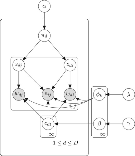
Then, we have $p(e_{w_{di},w_{dj}}=1)={\phi }_{c_{d{z}_{di}}}\cdot {\phi }_{c_{d{z}_{dj}}}.$

The principle of edge generation in HDP–GTM is consistent with GTM, assuming that there is association between words with similar topic distribution, and the similarity of topic distribution is determined by the inner product of the topic distribution of corresponding words.

In the HDP–GTM, the joint likelihood of the whole corpus is (:9) $\begin{array}{rl}& P(\mathbf{W},\mathbf{E},\mathbf{Z},\mathbf{\Theta }|\alpha ,\gamma ,\lambda )\\ & =\left\{\prod _{d=1}^D\prod _{k=1}^{\mathrm{\infty }}\prod _{t=1}^{\mathrm{\infty }}P\left({\mathit{\pi }}_d|\alpha \right)P\left(c_{dt}|\mathit{\beta }\right)P\left(\beta {{}^{\prime }}_k|\gamma \right)P\left({\phi }_k^{\mathrm{\prime }}|\lambda \right)\phantom{\left[\prod _{n=1}^{N_d}P(w_{dn}|z_{dn},\{{\phi }_k{\}}_{k=1}^{\mathrm{\infty }},c_{dt}\left)P\right(z_{dn}|{\mathit{\pi }}_d)\right]\prod _{i,j}\left[P\right(e_{w_{di},w_{dj}}\left)\right]}\right.\\ & \times \left[\prod _{n=1}^{N_d}P(w_{dn}|z_{dn},\{{\phi }_k{\}}_{k=1}^{\mathrm{\infty }},c_{dt}\left)P\right(z_{dn}|{\mathit{\pi }}_d)\right]\\ & \times \left.\prod _{i,j}\left[P\right(e_{w_{di},w_{dj}}\left)\right]\right\},\end{array}$(:9) where $\mathbf{\Theta }=(\mathit{\pi },\mathit{\beta },\mathit{\phi },\mathit{C})$, $\mathbf{W}=\left\{w_{dn}\right\}$, $\mathbf{E}=\left\{e_{w_{di},w_{dj}}\right\}$, $\mathbf{Z}=\left\{z_{dn}\right\}$, $\mathit{\pi }=\left\{{\pi }_d^{\prime }\right\}$, $\mathit{\beta }=\left\{{\beta }_k^{\prime }\right\}$ and $\mathit{c}=\left\{c_{dt}\right\}$.

4. Posterior inference for the HDP–GTM

In this section, we turn our attention to the procedures of posterior inference of the HDP–GTM. The key inferential problem we need to solve is the posterior distribution of latent variables given documents when we use probabilistic topic models. The posterior distribution for the HDP–GTM topic model is (10) $P(\mathbf{Z},\mathbf{\Theta }|\mathbf{W},\mathbf{E}).$(10) For nonparametric models, exact inference of the model parameters is intractable in general. In order to solve this problem, we discuss variational Bayes (VB) inference methods for the HDP–GTM. VB presents an efficient approximate method for the true posterior $P(\mathbf{Z},\mathbf{\Theta }|\mathbf{W},\mathbf{E})$ by minimising $KL\left(Q||P\right)$. Q is called variational distribution which is a simplification of the true posterior $P(\mathbf{Z},\mathbf{\Theta }|\mathbf{W},\mathbf{E})$. We propose the following factorised family of variational distributions for mean-field variational inference: (11) $\begin{array}{rl}Q(\mathit{Z},\mathbf{\Theta })& =\prod _{k=1}^{K-1}q({\beta }_k^{\mathrm{\prime }}|a_{k1},a_{k2})\prod _{k=1}^{K}q\left({\phi }_k|{\kappa }_k\right)\\ & \times \prod _{d=1}^D\left[\prod _{t=1}^{\mathrm{T}}q\left(c_{dt}|{\eta }_{dt}\right)\prod _{t=1}^{T-1}q({\pi }_{dt}^{\mathrm{\prime }}|{\gamma }_{dt1},{\gamma }_{dt2})\right.\\ & \times \left.\prod _{n=1}^{N}q\left(z_{dn}|{\zeta }_{dn}\right)\right],\end{array}$(11) where (12) $\begin{array}{rl}& {\beta }_k^{\mathrm{\prime }}\sim \mathrm{Beta}(a_{k1},a_{k2}),{\phi }_k\sim \mathrm{Dir}\left({\kappa }_k\right),\\ & c_{dt}\sim \mathrm{Multi}\left({\eta }_{dt}\right),{\pi }_{dt}^{\mathrm{\prime }}\sim \mathrm{Beta}({\gamma }_{dt1},{\gamma }_{dt2}),\\ & z_{dn}\sim \mathrm{Multi}\left({\zeta }_{dn}\right).\end{array}$(12) Let Σ be the set of the parameters in Equation (12(12) $\begin{array}{rl}& {\beta }_k^{\mathrm{\prime }}\sim \mathrm{Beta}(a_{k1},a_{k2}),{\phi }_k\sim \mathrm{Dir}\left({\kappa }_k\right),\\ & c_{dt}\sim \mathrm{Multi}\left({\eta }_{dt}\right),{\pi }_{dt}^{\mathrm{\prime }}\sim \mathrm{Beta}({\gamma }_{dt1},{\gamma }_{dt2}),\\ & z_{dn}\sim \mathrm{Multi}\left({\zeta }_{dn}\right).\end{array}$(12) ), then (13) $\begin{array}{rl}\mathrm{KL}\left(Q||P\right)& =E_Q\left[\mathsf{l}\mathsf{o}\mathsf{g}Q\right(\mathbf{Z},\mathbf{\Theta }\left)\right]-E_Q\left[\mathsf{l}\mathsf{o}\mathsf{g}P\right(\mathbf{Z},\mathbf{\Theta }|\mathbf{W},\mathbf{E})\\ & =E_Q\left[\mathsf{l}\mathsf{o}\mathsf{g}Q\right(\mathbf{Z},\mathbf{\Theta }\left)\right]-E_Q\left[\mathsf{l}\mathsf{o}\mathsf{g}P\right(\mathbf{Z},\mathbf{\Theta },\mathbf{W},\mathbf{E}\left)\right]\\ & +\mathsf{l}\mathsf{o}\mathsf{g}P(\mathbf{W},\mathbf{E}).\end{array}$(13) Let (14) $L\left(\mathrm{\Sigma }\right)=E_Q\left[\mathsf{l}\mathsf{o}\mathsf{g}P\right(\mathbf{Z},\mathbf{\Theta },\mathbf{W},\mathbf{E}\left)\right]-E_Q\left[\mathsf{l}\mathsf{o}\mathsf{g}Q\right(\mathbf{Z},\mathbf{\Theta }\left)\right],$(14) where $L\left(\mathrm{\Sigma }\right)$ is called the evidence lower bound (ELBO) which is dependent on the variational parameters Σ. The goal is to minimise the objective function $\mathrm{KL}$-divergence which is equivalent to maximise the evidence lower bound function. We use truncations for inferencing the number of factors at T and K. Having specified a simplified family of probability distributions, the next step is to set up an optimisation problem that determines the values of the variational parameters. The derivation details can be found in Appendix 1. For document-level updates, at the document level we update the parameters to the per-document stick, and the parameters are (15) $\begin{array}{rl}{a}_{k1}& =1+\sum _{d=1}^D\sum _{t=1}^{\mathrm{T}}{\eta }_{dtk},\\ a_{k2}& =\gamma +\sum _{d=1}^D\sum _{t=1}^{\mathrm{T}}\sum _{f=k+1}^K{\eta }_{dtk},\\ {\eta }_{dtk}& =\exp \left\{\sum _{e=1}^{k-1}\left(\mathrm{\Psi }\right(a_{e2})-\mathrm{\Psi }(a_{e1}+a_{e2}\left)\right)\right.\\ & +\left(\mathrm{\Psi }\right(a_{k1})-\mathrm{\Psi }(a_{k1}+a_{k2}\left)\right)\phantom{\left(\mathrm{\Psi }\left({\lambda }_{kv}\right)-\mathrm{\Psi }\left(\sum _{l=1}^V{\lambda }_{kl}\right)\right)}+\sum _{n=1}^N\sum _{v=1}^V\\ & \left.w_{dn}^v{\zeta }_{dnt}\left(\mathrm{\Psi }\left({\lambda }_{kv}\right)-\mathrm{\Psi }\left(\sum _{l=1}^V{\lambda }_{kl}\right)\right)\right\}.\end{array}$(15) There exists no closed-form solution for ${\zeta }_{dtk}$. We can derive Iterative expression of ${\zeta }_{dtk}$ by the Newton's method. (16) ${\zeta }_{dtk}^{(n+1)}={\zeta }_{dtk}^{\left(n\right)}-H\left({\zeta }_{dtk}^{\left(n\right)}{)}^{-1}{\mathrm{\Delta }}_{{\zeta }_{dtk}^{\left(n\right)}}L\right({\zeta }_{dtk}^{\left(n\right)}),$(16) where $f\left({\zeta }_{dtk}^{\left(n\right)}\right)$ and $H\left({\zeta }_{dtk}^{\left(n\right)}\right)$ are provided in Appendix 1. At the corpus level, we update the parameters to top-level sticks and the topics, (17) $\begin{array}{rl}{\gamma }_{dt1}& =1+\sum _{n=1}^N{\zeta }_{dnt},\\ {\gamma }_{dt2}& ={\alpha }_0+\sum _{n=1}^N\sum _{b=t+1}^{\mathrm{T}}{\zeta }_{dnt},\\ {\kappa }_{jv}& ={\beta }_{jv}+\sum _{d=1}^D\sum _{n=1}^{N_d}{w}_{dn}^v{\zeta }_{dnt}{\eta }_{dtk}.\end{array}$(17) For each iterative step, define (18) ${\mathrm{\Sigma }}^{\left(n\right)}=M\left({\mathrm{\Sigma }}^{(n-1)}\right),$(18) for $n=1,\dots ,$ where M denotes a certain mapping and $\left\{{\mathrm{\Sigma }}^{\left(n\right)}\right\}$ denotes the sequences of iterates that are produced. To verify the convergence of Algorithm 1, we need to combine Wang and Titterington (2006) and the convergence of the Newton's method. Therefore, by Theorem 1 of Wang and Titterington (2006), we have the following theorem, of which a proof is given in Appendix 2.

Theorem 4.

as n approaches infinity, the iterative procedure (18(18) ${\mathrm{\Sigma }}^{\left(n\right)}=M\left({\mathrm{\Sigma }}^{(n-1)}\right),$(18) ) with probability 1 converges locally to the true value ${\mathrm{\Sigma }}^{\star };$ that is, the iterative procedure (18(18) ${\mathrm{\Sigma }}^{\left(n\right)}=M\left({\mathrm{\Sigma }}^{(n-1)}\right),$(18) ) converges to the true value ${\mathrm{\Theta }}^{\star }$ and the starting values are sufficiently near to ${\mathrm{\Sigma }}^{\star }$.

5. Experiments

This section mainly carries out experimental design and verifies the superiority of new model HDP–GTM proposed in the previous section. The organisational structure of this section is as follows: first, the dataset used in this experiment is explained, including the preprocessing of the dataset. Then the design scheme is tested, Support Vector Machine (SVM) algorithm is adopted to classify the text, and indicators to evaluate the experimental results are given. Finally, the text classification effects of HDP–GTM, GTM, HDP and LDA are compared.

5.1. Data description

Two text libraries were used in this chapter experiment, Reuters-21578¹ and 20-newsgroup². Reuters-21578 is a series of news articles published on Reuters news website in 1987. It is widely used in text classification tasks and has been manually marked by Reuters personnel. This group consists of 21,578 documents, some of which are unmarked, and some of which are marked with one or more of 672 different categories. These categories are divided into five different categories: communication, organisation, personnel, location and theme. The 20-newsgroup data set is a news text library, which is often used for text classification, text mining and information retrieval. This text library integrates about 20,000 news texts, and is evenly divided into 20 collections according to different news themes.

Before text analysis, the dataset should be preprocessed first. The main purpose of text preprocessing is to reduce the dimension of the text data by controlling vocabulary so as to analyse the subsequent process. Text preprocessing steps commonly used in text classification are tagging, normalisation, stop-word removal and word stem.

• Tagging: based on the ‘bag of words’ assumptions, the text is divided into words or other meaningful parts regardless of the order between words. After being split, the whole text library is like a bag filled with words, and each word will correspond to a unique code.

• Normalisation: To convert and add or delete words in the document such as changing all uppercase parts of words into lowercase, discarding words with vocabulary less than 10 words in articles, discarding words with vocabulary less than 3 or more than 20 characters, deleting numbers and non-alphabetic characters, etc.

• Delete stop words: Stop words refer to words that are often encountered in the text but have nothing to do with analysis, such as prepositions, articles, conjunctions and so on.

• Words stem: Stemming is used to identify the root/stem of a word in the text.

After preprocessing, the variance threshold of a simple baseline method is adopted to select features, and the features whose variance does not meet the threshold are removed. In the traditional theme model, we get the document vector through the ‘bag of words’ (Aldous, 1985). Word bag is a simplified representation in which documents are represented by word bag regardless of grammar or even word order.

This paper studies the text data of graph structure at the word level and considers the co-occurrence relationship between words. Therefore, before applying the theme model HDP–GTM, we also need to calculate the correlation coefficient between words and convert the text data into graph structure data. On the basis of traditional data preprocessing, it is necessary to add one step operation at the last step to convert text data into graph structure data. First, according to the following formula: (19) $f_{co}=\frac{|N_{e_i}\cap N_{e_j}|}{|D|},$(19) where D is the number of documents in the corpus, $N_{e_i}$ and $N_{e_j}$ denote the number of words $e_i$ and $e_j$ in the corpus D respectively. We need to calculate the frequency of common occurrence of each pair of words $f_{CO}$, and then compare it with the preset threshold ρ, to determine whether there are edges between words. If $f_{co}(i,j)\ge \rho$, the results of parameter derivation in the previous chapter show that the existence of edges will affect the calculation of posterior parameters.

5.2. Experiment design

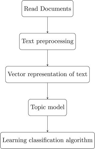
The ‘bag of words’ representations of the documents are unable to recognise synonyms from a given term set and unable to recognise semantic relationships between terms. We apply the topic-model approach to cluster the words into a set of topics. Words assigned into the same topic are semantically related. Our main goal is to compare the performance of classification among different topic models. We also apply and compare whether the different threshold values have effects on the classification. This experimental process is divided into three stages, text preprocessing stage, topic models training stage and text classification stage(Figure 5).

Figure 5. Graphical model representation of the process for text classification.

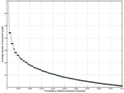
In the topic models training stage, all documents are used to train the topic model, and the purpose is to extract valid feature information of the text. In the text classification stage, the text set is divided into training set and test set, and support vector machine (SVM) is adopted to classify the text trained by different topic models, and the classification effect of different models under SVM is compared. Because we consider the association between words in the graph theme model, it is necessary to set the threshold value to determine whether edges exist or not in advance before experiments are carried out. When we set different thresholds ρ, the number of edges existing in the text is different. Figure 6 shows the relationship between threshold and average graph density in the Reuters dataset.

Figure 6. The relation between threshold value of word relation and average graph density.

5.3. Evaluation measures

In this paper, accuracy, recall and F-score are selected as evaluation index of experimental results. Accuracy and recall are often used in the fields of information retrieval and text mining as important indicators to test model results. As far as text classification is concerned, accuracy is used to measure the number of correctly classified texts in the extracted texts accounting for the number of samples. The recall is the proportion of correctly classified samples to all samples in the sample. In Table 1, TP indicates the actual number of samples in class a which are finally assigned to class a, FP indicates the actual number of samples in class b which are predicted as the class a, FN indicates the actual number of samples in class a which are predicted as class b and TN indicates the actual number of samples in class b which are predicted as the class b. The calculation formula of the precision rate is $P=TP/(TP+FP)$. The calculation formula of the recall rate is $R=TP/(TP+FN)$. In the actual classification, we hope that the higher the value of P is, the better it is, and the higher the value of R is, but sometimes when p and r values conflict, we can refer to the value of F at this time. F is a harmonic average of accuracy and recall $F=2PR/(P+R)$. The larger F is, the better the classification effect.

5.4. Result analysis

The subject categories belong to which in Reuters data set and 20-newsgroup data set are known. At the beginning of the experiment, first, the topic distribution of each document is deduced by HDP–GTM, HDP, GTM and LDA models, and then SVM algorithm is applied to classify the topic of each document. Finally, the classification effect of different models is compared by calculating the classification accuracy and recall rate. We set different correlation coefficient threshold ρ and use SVM classification method to compare the text topic classification effects of HDP–GTM and other three models HDP, GTM and LDA.

Table 1. Evaluation measures.

	True classification	False classification
Predicted true classification	TP (true positive)	FP (false positive)
Predicted false classification	FN (false negative)	TN (true negative)

5.4.1. Reuter dataset

The Reuters data set is preprocessed, and finally 8025 texts are left. In the process of SVM text classification, 5770 of these texts are used as training sets, and the rest 2255 documents are used as test sets. In this experiment, four thresholds ρ are selected to compare the precision, recall and $F_1$ value of topic classification of Reuters dataset by three models under different thresholds.

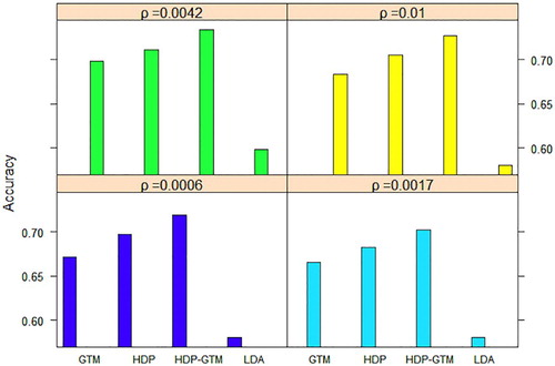
From Table 2, the classification accuracy of HDP–GTM is generally higher than that of other three models. The selection of the average density threshold ρ of the graph basically has no influence on the classification effect of LDA and HDP, because LDA and HDP models are based on the ‘bag of words’ assumption, and the correlation between words is not considered, so the classification accuracy of LDA and HDP is not different in different graph densities. GTM and HDP–GTM are relatively sensitive to average plot density, but it is not that the larger the plot density, the better. As shown in Figure 7, when $\rho =0.0042$, HDP–GTM has the best classification effect, and the figure density at this time is 0.4017.

Figure 7. Classification effect of Reuters dataset under different ρ.

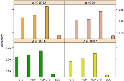
Table 2. Classification effects of the Reuters.

Reuters dataset
	$\rho =0.01$				$\rho =0.0042$
	HDP–GTM	HDP	GTM	LDA	HDP–GTM	HDP	GTM	LDA
P	$\mathbf{0}.\mathbf{742}$	0.708	0.705	0.582	$\mathbf{0}.\mathbf{763}$	0.714	0.714	0.588
R	$\mathbf{0}.\mathbf{904}$	0.878	0.880	0.580	$\mathbf{0}.\mathbf{920}$	0.876	0.884	0.600
F	$\mathbf{0}.\mathbf{818}$	0.784	0.783	0.566	$\mathbf{0}.\mathbf{834}$	0.794	0.790	0.562
	$\rho =0.0017$				$\rho =0.0006$
	HDP–GTM	HDP	GTM	LDA	HDP–GTM	HDP	GTM	LDA
P	$\mathbf{0}.\mathbf{725}$	0.707	0.690	0.580	$\mathbf{0}.\mathbf{737}$	0.716	0.710	0.581
R	$\mathbf{0}.\mathbf{888}$	0.881	0.885	0.582	$\mathbf{0}.\mathbf{900}$	0.873	0.876	0.583
F	$\mathbf{0}.\mathbf{798}$	0.781	0.775	0.564	$\mathbf{0}.\mathbf{811}$	0.786	0.784	0.568

5.4.2. 20-newsgroup dataset

The 20-news group data set has 18,846 documents left after data preprocessing. In the process of SVM text classification, 11,314 documents are used as test sets, and the rest 7532 documents are used as test sets. In order to compare the topic classification effects of the three models for the text library, the thresholds in this section are consistent with those in the previous section. Table 3 shows the classification effect of three different models under different thresholds. Overall, the classification effect of HDP–GTM model is better than that of other three models.

Table 3. Classification effects of the 20-newsgroup.

20-newsgroup dataset
	$\rho =0.01$				$\rho =0.0042$
	HDP–GTM	HDP	GTM	LDA	HDP–GTM	HDP	GTM	LDA
P	0.727	0.702	0.683	0.581	0.702	0.698	0.665	0.580
R	0.823	0.813	0.848	0.734	0.815	0.802	0.798	0.723
$F_1$	0.772	0.755	0.757	0.684	0.754	0.748	0.725	0.681
	$\rho =0.0017$				$\rho =0.0006$
	HDP–GTM	HDP	GTM	LDA	HDP–GTM	HDP	GTM	LDA
P	0.734	0.695	0.698	0.598	0.719	0.697	0.671	0.580
R	0.873	0.811	0.858	0.735	0.835	0.809	0.816	0.776
$F_1$	0.754	0.751	0.725	0.681	0.796	0.751	0.770	0.697

Comparing the classification results of Table 3, we can find that the classification accuracy of LDA and HDP model for two datasets is not different which indicates that LDA and HDP modes are relatively stable for topic classification. At the same time, the sensitivity of the two datasets to the threshold is different. As shown in Figure 8, HDP–GTM performs best when $\rho =0.0006$.

Figure 8. Classification effect of 20-newsgroup dataset under different ρ.

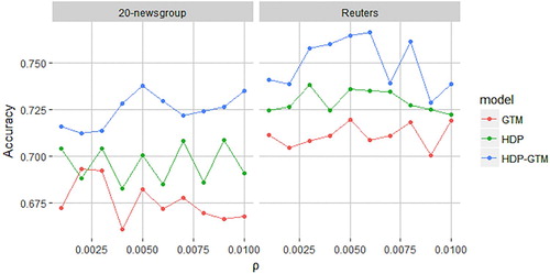
5.5. Selection of the threshold

For graph structure data, the selection of threshold value is related to the number of edges in the graph, and the range of threshold value is $\rho \in (0,1)$. Consider the extreme situation: when ρ approaches zero, it means that the density of the graph approaches 1, that is to say, this graph is a connected graph, that is, there are edges between each pair of node pairs. When $\rho =0$, it means that two nodes appear simultaneously in every document, which is almost impossible in practice. The edges in the graph are almost zero, and HDP–GTM at this time is equivalent to the HDP model and the GTM at this time is equivalent to the LDA model.

Through the analysis of the above two data sets, it is found that the accuracy of GTM and HDP–GTM model for the topic classification of Reuters data set is higher than that of 20-newsgroup data set, as shown in Figure 9. This difference is mainly related to the data structure of the database itself. Figure 9 shows the classification effect of GTM model and HDP–GTM model on two datasets.

Figure 9. Classification effect of two datasets under HDP–GTM model.

6. Discussion

This paper proposed a new method HDP–GTM for probabilistic topic modelling. HDP–GTM takes advantage of the HDP and the GTM. We applied a variational inference algorithm for calculating the posterior distribution and investigated its convergence property. In the experimental analysis, we reported applications in text categorisation of the Reuters dataset and the 20 newsgroup data set by the HDP–GTM, compared to HDP, GTM and LDA. We found that the HDP–GTM is better than HDP, GTM and LDA. Future researches can be considered from the following aspects:

1. The graph structure in this paper considers the co-occurrence relationship at the word level, and it is not widely used in terms of the research scope. In addition to co-occurrence relations, future research can consider other related relations, such as proximity relations, semantic relations (Griffiths et al., 2005).

2. Besides considering the graph structure at the word level, we can also try other graph structures at other levels, such as the graph structure at the topic level or the graph structure at the document level.

3. This paper considers the HDP for the prior distribution of topics, besides, other nonparametric Bayesian processes can be also considered, such as the Pitman–Yor process (Sato & Nakagawa, 2010).

Disclosure statement

No potential conflict of interest was reported by the authors.

Additional information

Funding

This research was supported by NSFC under grant No. 71371074 and the 111 Project under No. B14019.

Notes on contributors

Haibin Zhang

Haibin Zhang is currently pursuing the doctoral degrees from East China normal University, Shanghai, China. His current research interests include text mining, machine learning, and deep learning.

Shang Huating

Huating Shang received the master’s degree from East China normal University. She is a statistical analyst in Jiangsu Hengrui Medicine. Her current research interests include text mining and clinical trial.

Xianyi Wu

Xianyi Wu received the PH.D degree from East China normal University. He is a professor with school of statistics, East China normal University. His current research interests include mathematical statistics actuarial, stochastic scheduling and machine learning.

Notes

1 http://www.davidlewis.com/resources/testcollections/Reuters21578/.

2 http://www.qwone.com/Jason/20newsgroups/.

Appendices

Appendix 1. Derivation of posterior inference for GTM–HDP

First, we expand evidence lower bound function $L\left(\mathrm{\Sigma }\right)$, $\begin{array}{rl}L\left(\mathrm{\Sigma }\right)& =E_Q\left[\mathsf{l}\mathsf{o}\mathsf{g}P\right(\mathbf{Z},\mathbf{\Pi },\mathit{\beta },\mathit{C},\mathbf{W},\mathbf{E}|\alpha ,\gamma ,\lambda \left)\right]\\ & -E_Q\left[\mathsf{l}\mathsf{o}\mathsf{g}Q\right({\mathit{\beta }}^{\mathrm{\prime }},{\mathit{\phi }}^{\mathrm{\prime }},{\mathit{\pi }}^{\mathrm{\prime }},{\mathit{C}}^{\mathrm{\prime }},{\mathit{Z}}^{\mathrm{\prime }}\left)\right]\\ & =\sum _{d=1}^D\left[E_Q\mathsf{l}\mathsf{o}\mathsf{g}P\right({\mathit{\pi }}_d|\alpha )+\sum _{t=1}^{\mathrm{\infty }}{E}_Q\mathsf{l}\mathsf{o}\mathsf{g}P(c_{dt}|\mathit{\beta })\\ & +\sum _{n=1}^{N_d}\sum _{t=1}^{\mathrm{\infty }}\sum _{k=1}^{\mathrm{\infty }}{E}_Q\mathsf{l}\mathsf{o}\mathsf{g}P(w_{dn}|z_{dn},{\phi }_k,c_{dt})\\ & +\sum _{n=1}^{N_d}{E}_Q\mathsf{l}\mathsf{o}\mathsf{g}P\left(z_{dn}|{\mathit{\pi }}_d\right)+\sum _{i,j}{E}_Q\mathsf{l}\mathsf{o}\mathsf{g}P\left(e_{w_{di},w_{dj}}\right)]\\ & +\sum _{k=1}^{\mathrm{\infty }}{E}_Q\mathsf{l}\mathsf{o}\mathsf{g}P\left({\beta }_k|\gamma \right)+\sum _{k=1}^{\mathrm{\infty }}{E}_Q\mathsf{l}\mathsf{o}\mathsf{g}P\left({\phi }_k|{\lambda }_k\right)\\ & -\sum _{d=1}^D\left[\sum _{t=1}^{\mathrm{\infty }}q({\pi }_{dt}|{\gamma }_{dt}^1,{\gamma }_{dt}^2)-\sum _{t=1}^{\mathrm{\infty }}q\left(c_{dt}|{\zeta }_{dt}\right)\right.\\ & \left.-\sum _{n=1}^{N_d}{E}_Q\mathsf{l}\mathsf{o}\mathsf{g}P\left(z_{dn}|{\mathit{\phi }}_d\right)\right]\\ & +\sum _{k=1}^{\mathrm{\infty }}{E}_Q\mathsf{l}\mathsf{o}\mathsf{g}q({\beta }_k|a_k^1,a_k^2)+\sum _{k=1}^{\mathrm{\infty }}{E}_Q\mathsf{l}\mathsf{o}\mathsf{g}q\left({\phi }_k|{\lambda }_k\right).\end{array}$ We rewrite the first term using indicator random variables: $\begin{array}{rl}& E_{q\left({\mathit{\pi }}_{\mathbf{\text{d}}}\right)}\mathsf{l}\mathsf{o}\mathsf{g}\mathsf{P}\mathsf{\left(}{\pi }_{\mathsf{d}\mathsf{t}}\mathsf{|}\alpha \mathsf{\right)}\\ & =\sum _{s=1}^{t-1}{E}_{q\left({\pi }_{\mathbf{\text{d}}}\right)}\mathsf{l}\mathsf{o}\mathsf{g}(1-{\pi }_{ds}^{\mathrm{\prime }})+E_{q\left({\pi }_{\mathbf{\text{d}}}\right)}\mathsf{l}\mathsf{o}\mathsf{g}\mathsf{\left(}{\pi }_{\mathsf{d}\mathsf{t}}^{\mathrm{\prime }}\mathsf{\right)}\mathsf{,}\end{array}$ where $\begin{array}{rl}{E}_{q\left({\pi }_{\mathbf{\text{d}}}\right)}\left[\mathsf{l}\mathsf{o}\mathsf{g}{\pi }_{dt}^{\mathrm{\prime }}\right]& =\mathrm{\Psi }\left({\gamma }_{dt1}\right)-\mathrm{\Psi }(\gamma dt1+{\gamma }_{dt2}),\\ E_{q\left({\pi }_{\mathbf{\text{d}}}\right)}\left[\mathsf{l}\mathsf{o}\mathsf{g}\right(1-{\pi }_{dt}^{\mathrm{\prime }}\left)\right]& =\mathrm{\Psi }\left({\gamma }_{dt2}\right)-\mathrm{\Psi }({\gamma }_{dt1}+{\gamma }_{dt2}).\end{array}$ The digamma function, denoted by Ψ, arises from the derivative of the log normalisation factor in the beta distribution. Then, $\begin{array}{rl}& E_{q\left({\pi }_{\mathbf{\text{d}}}\right)}\mathsf{l}\mathsf{o}\mathsf{g}\mathsf{P}\mathsf{\left(}{\pi }_{\mathsf{d}\mathsf{t}}\mathsf{|}\alpha \mathsf{\right)}\\ & =\left\{\begin{array}{ll}\sum _{s=1}^{t-1}{E}_{q\left({\pi }_{\mathbf{\text{d}}}\right)}\mathsf{l}\mathsf{o}\mathsf{g}\mathsf{(}\mathsf{1}\mathsf{-}{\pi }_{\mathsf{d}\mathsf{s}}^{\mathrm{\prime }}\mathsf{)}\mathsf{+}{\mathsf{E}}_{\mathsf{q}\mathsf{\left(}{\pi }_{\mathbf{\text{d}}}\mathsf{\right)}}\mathsf{l}\mathsf{o}\mathsf{g}\mathsf{\left(}{\pi }_{\mathsf{d}\mathsf{t}}^{\mathrm{\prime }}\mathsf{\right)}& \mathrm{if}t<T,\\ \sum _{s=1}^{T-1}{E}_{q\left({\pi }_{\mathbf{\text{d}}}\right)}\mathsf{l}\mathsf{o}\mathsf{g}\mathsf{(}\mathsf{1}\mathsf{-}{\pi }_{\mathsf{d}\mathsf{s}}^{\mathrm{\prime }}\mathsf{)}& \mathrm{if}t\ge T.\end{array}\right.\\ & E_Q\log P\left(z_{dn}|{\pi }_d\right)=\sum _{t=1}^{\mathrm{\infty }}q(z_{dn}=t)E_Q\left[\mathsf{l}\mathsf{o}\mathsf{g}\mathsf{P}\mathsf{\right(}{\pi }_{\mathsf{d}\mathsf{t}}\mathsf{\left)}\mathsf{\right]}\mathsf{.}\end{array}$ Recall that $q(z_{dn}=t)=0$ for $t\ge T$. Consequently, we can truncate this summation at t=T: $E_{Q(\mathbf{Z},\mathbf{\Theta })}\log P\left(z_{dn}\right)=\sum _{t=1}^{T-1}q(z_{dn}=t)E_Q\left[\mathsf{l}\mathsf{o}\mathsf{g}P\right({\pi }_{dt}\left)\right],$ where $q(z_{dn}=t)={\tilde{\pi }}_{dt}$. Similarly, $\begin{array}{rl}& E_{q\left({\beta }_{\mathbf{\text{k}}}\right)}\mathsf{l}\mathsf{o}\mathsf{g}P\left({\beta }_k|\gamma \right)\\ & =\left\{\begin{array}{ll}\sum _{\ell =1}^{k-1}{E}_{q\left({\beta }_{\mathbf{\text{k}}}\right)}\mathsf{l}\mathsf{o}\mathsf{g}(1-{\beta }_{\ell }^{\mathrm{\prime }})+E_{q\left({\beta }_{\mathbf{\text{l}}}\right)}\mathsf{l}\mathsf{o}\mathsf{g}\left({\beta }_{\ell }^{\mathrm{\prime }}\right)& \text{if }k<K,\\ \sum _{k=1}^{K-1}{E}_{q\left({\beta }_{\mathbf{\text{k}}}\right)}\mathsf{l}\mathsf{o}\mathsf{g}(1-{\beta }_{\ell }^{\mathrm{\prime }})& \text{if }k\ge K,\end{array}\right.\end{array}$ where $\begin{array}{rl}{E}_q\left[\mathsf{l}\mathsf{o}\mathsf{g}{\beta }_k^{\mathrm{\prime }}\right]& =\mathrm{\Psi }\left(a_{k1}\right)-\mathrm{\Psi }(a_{k1}+a_{k2}),\\ E_q\left[\mathsf{l}\mathsf{o}\mathsf{g}\right(1-{\beta }_k^{\mathrm{\prime }}\left)\right]& =\mathrm{\Psi }\left(a_{k2}\right)-\mathrm{\Psi }(a_{k1}+a_{k2}),\\ E_Q\mathsf{l}\mathsf{o}\mathsf{g}P\left(c_{dt}|\mathit{\beta }\right)& =\sum _{k=1}^{K-1}q(c_{dt}=k)E_q\left[\mathsf{l}\mathsf{o}\mathsf{g}{\beta }_k\right],\end{array}$ where $q(c_{dt}=k)={\eta }_{dtk}$. $\begin{array}{rl}& E_Q\log P\left({\phi }_{\mathit{k}}|{\lambda }_{\mathit{k}}\right)\\ & =\sum _{v=1}^V({\lambda }_{kv}-1)\left(\mathrm{\Psi }\left({\kappa }_{jv}\right)-\mathrm{\Psi }\left(\sum _{k=1}^V{\kappa }_{jk}\right)\right)\\ & +\log \left(\mathrm{\Gamma }\left(\sum _{v=1}^V{\lambda }_{kv}\right)\right)-\sum _{v=1}^V\log \left(\mathrm{\Gamma }\right({\lambda }_{kv}\left)\right),\\ & E_Q\mathsf{l}\mathsf{o}\mathsf{g}P(w_{dn}|z_{dn},{\phi }_k,c_{dt})\\ & =\sum _{k=1}^{\mathrm{T}}\sum _{v=1}^{V}q(z_{dn}=t)w_{dn}^v{\eta }_{dtk}{E}_{Q(\mathbf{Z},\mathrm{\Theta })}\left[\log \right({\phi }_{jv}\left)\right].\end{array}$ To simplify our notation, let $w_{dn}^v=1$, iff $w_{dn}$ is the vth word in the vocabulary. $\begin{array}{rl}q(z_{dn}=t)& ={\zeta }_{dtk},\\ E_Q\left[\log {\phi }_{kv}\right]& =\mathrm{\Psi }\left({\lambda }_{kv}\right)-\mathrm{\Psi }\left(\sum _{k=1}^V{\lambda }_{kv}\right),\\ \sum _{(i,j)}{E}_q\left[\mathsf{l}\mathsf{o}\mathsf{g}p\left(e_{w_{di},w_{dj}}\right)\right]& =\sum _{(i,j)}{E}_q\left[\mathsf{l}\mathsf{o}\mathsf{g}({\phi }_{c_{d{z}_{di}}}\cdot {\phi }_{c_{d{z}_{dj}}})\right]\\ & \approx \sum _{(i,j)}{E}_q\left[{\varsigma }^{-1}\sum _k^K{\phi }_{di,k}.{\phi }_{dj,k}\right.\\ & \left.\phantom{\approx \sum _{(i,j)}{E}_q\left[{\varsigma }^{-1}\sum _k^K{\phi }_{di,k}.{\phi }_{dj,k}\right.}+\mathsf{l}\mathsf{o}\mathsf{g}\varsigma -1\right]\\ & =\sum _{(i,j)}\left({\varsigma }^{-1}{\lambda }_{ki}^{{\phi }_{dik}}.{\lambda }_{kj}^{{\phi }_{dik}}+\mathsf{l}\mathsf{o}\mathsf{g}\varsigma -1\right).\\ \varsigma & =N_{(i,j)}\sum _k^K({\lambda }_{k,n_i}^{{\varphi }_{d,n_i,k}}\cdot {\lambda }_{k,n_j}^{{\varphi }_{d,n_j,k}}).\end{array}$ It can be seen from the forming process of edge that the probability of edge existence follows a binomial distribution, which is obtained by the inner product of the word distribution of the corresponding node subject. The above second step uses the Taylor's expansion of the logarithmic function at the point ς.

We first maximise equation with respect to ${\eta }_{dtk}$. Observe that this is a constrained maximisation since $\sum _{k=1}^K{\eta }_{dtk}=1$. We form the Lagrangian by isolating the terms which contain ${\eta }_{dtk}$ and adding the appropriate Lagrange multipliers. $\begin{array}{rl}{L}_{\left[{\eta }_{dtk}\right]}& ={\eta }_{dtk}{E}_{q\left(\beta \right)}\mathsf{l}\mathsf{o}\mathsf{g}\left({\beta }_{\ell }^{\mathrm{\prime }}\right)+{\eta }_{dtk}{E}_{q\left(\beta \right)}\mathsf{l}\mathsf{o}\mathsf{g}(1-{\beta }_{\ell }^{\mathrm{\prime }})\\ & -{\eta }_{dtk}\log \left({\eta }_{dtk}\right)+\lambda \left(\sum _{i=1}^{\mathrm{T}}{\eta }_{dtk}-1\right)\\ & ++\sum _{n=1}^N\sum _{v=1}^V{w}_{dn}^v{\eta }_{dtk}{\zeta }_{dnt}\left(\mathrm{\Psi }\right({\lambda }_{kv})-\mathrm{\Psi }\left(\sum _{l=1}^V{\lambda }_{kl}\right).\end{array}$

Taking derivatives with respect to ${\eta }_{dtk}$ and setting this derivative to zero yields the maximising value of the variational parameter ${\eta }_{dtk}$, we obtain $\begin{array}{rl}{\eta }_{dtk}& =\exp \left\{\sum _{e=1}^{k-1}\left(\mathrm{\Psi }\right(a_{e2})-\mathrm{\Psi }(a_{e1}+a_{e2}\left)\right)+\left(\mathrm{\Psi }\right(a_{k1})\right.\\ & -\mathrm{\Psi }(a_{k1}+a_{k2}))\\ & \left.+\sum _{n=1}^N\sum _{v=1}^V{w}_{dn}^v{\zeta }_{dnt}\left(\mathrm{\Psi }\left({\lambda }_{kv}\right)-\mathrm{\Psi }\left(\sum _{l=1}^V{\lambda }_{kl}\right)\right)\right\}.\end{array}$ Similarly, $\begin{array}{rl}{a}_{k1}& =1+\sum _{d=1}^D\sum _{t=1}^{\mathrm{T}}{\eta }_{dtk},a_{k2}=\gamma +\sum _{d=1}^D\sum _{t=1}^{\mathrm{T}}\sum _{f=k+1}^K{\eta }_{dtf},\\ {\gamma }_{dt1}& =1+\sum _{n=1}^N{\zeta }_{dnt},{\gamma }_{dt2}={\alpha }_0+\sum _{n=1}^N\sum _{b=t+1}^{\mathrm{T}}{\zeta }_{dnb},\\ {\kappa }_{jv}& ={\beta }_{jv}+\sum _{d=1}^D\sum _{n=1}^{N_d}{w}_{dn}^v{\zeta }_{dnt}{\eta }_{dtk}.\end{array}$ For the parameter ${\zeta }_{dnt}$, when finding the maximum value of $L\left({\zeta }_{dnt}\right)$ under the constraint of $\sum _t^{\mathrm{T}}{\zeta }_{dnt}=1)$, then the partial derivative of ${\zeta }_{dnt}$: $\begin{array}{rl}{\mathrm{\Delta }}_{{\zeta }_{dtk}}L\left({\zeta }_{dtk}\right)& =\left(\mathrm{\Psi }\left({\kappa }_{k,n}\right)-\mathrm{\Psi }\left(\sum _{n=1}^N{\kappa }_{k,n}\right)\right)\\ & +\sum _{h=1}^{k-1}\left(\mathrm{\Psi }\left({\gamma }_{dh2}\right)-\mathrm{\Psi }({\gamma }_{dh1}+{\gamma }_{dh2})\right)\\ & +\mathrm{\Psi }\left({\gamma }_{dk1}\right)-\mathrm{\Psi }({\gamma }_{dk1}+{\gamma }_{dk2})-\mathsf{l}\mathsf{o}\mathsf{g}{\zeta }_{d,n,k}-1\\ & +\sum _{n_j\in Ne\left(n_i\right)}({\varsigma }^{-1}\cdot \mathsf{l}\mathsf{o}\mathsf{g}{\kappa }_{k,n}\cdot {\kappa }_{k,n}^{{\zeta }_{d,n,k}})\\ & +\sum _{k=1}^N\sum _{v=1}^V{w}_{dn}^v{\eta }_{dtk}\left(\mathrm{\Psi }\left({\lambda }_{kv}\right)-\mathrm{\Psi }\left(\sum _{l=1}^V{\lambda }_{kl}\right)\right).\end{array}$ Then the second derivative of ${\zeta }_{dtk}$ is $H\left({\zeta }_{dtk}\right)=\mathrm{\partial }L/\mathrm{\partial }{\zeta }_{dtk}\mathrm{\partial }{\zeta }_{dtk}$, by Newton's method, ${\zeta }_{dtk}^{(n+1)}={\zeta }_{dtk}^{\left(n\right)}-H\left({\zeta }_{dtk}^{\left(n\right)}{)}^{-1}{\mathrm{\Delta }}_{{\zeta }_{dtk}^{\left(n\right)}}f\right({\zeta }_{dtk}^{\left(n\right)}).$

Appendix 2.

Proof of Theorem 4.1

We derived Σ into two parts ζ and the remaining part of Σ expressed by Γ, and note that ${\mathrm{\Gamma }}^{\star }$ and ${\zeta }^{\star }$ are the true value of Γ and ζ respectively. Then $\parallel \mathrm{\Sigma }-{\mathrm{\Sigma }}^{\star }\parallel =∥\left(\begin{array}{c}\mathrm{\Gamma }\\ \zeta \end{array}\right)-\left(\begin{array}{c}{\mathrm{\Gamma }}^{\star }\\ {\zeta }^{\star }\end{array}\right)∥=∥\left(\begin{array}{c}\mathrm{\Gamma }-{\mathrm{\Gamma }}^{\star }\\ \zeta -{\zeta }^{\star }\end{array}\right)∥,$ the convergence of $\parallel \mathrm{\Gamma }-{\mathrm{\Gamma }}^{\star }\parallel$ is a special case of Theorem 1 in Wang and Titterington (2006), then the iterative procedure converges to the true value ${\mathrm{\Gamma }}^{\star }$. The convergence of $\parallel \zeta -{\zeta }^{\star }\parallel$ can be proved by the Newton's method. With probability 1 as n approaches infinity, the iterative procedure (18(18) ${\mathrm{\Sigma }}^{\left(n\right)}=M\left({\mathrm{\Sigma }}^{(n-1)}\right),$(18) ) converges locally to the true value ${\mathrm{\Sigma }}^{\star }$.

References

- Aldous, D. J. (1985). Exchangeability and related topics. Berlin: Springer.
- Blackwell, D., & MacQueen, J. (1973). Ferguson distributions via Polya urn schemes. The Annals of Statistics, 1, 353–355. doi: 10.1214/aos/1176342372
- Blei, David M. (2012). Probabilistic topic models. Communications of the ACM, 55(4), 77–84. doi: 10.1145/2133806.2133826
- Blei, D. M., Kucukelbir, A., & McAuliffe, J. D. (2017). Variational inference: A review for statisticians. Journal of the American Statistical Association, 112(518), 859–877. doi:10.1080/01621459.2017.1285773
- Blei, D. M., Ng, A. Y., Jordan, M. I. (2003). Latent Dirichlet allocation. Journal of Machine Learning Research, 3, 993–1022.
- Deerwester, S. (1990). Indexing by latent semantic analysis. Journal of the Association for Information Science and Technology, 41(6), 391–407.
- Ferguson, T. S. (1973). A Bayesian analysis of some nonparametric problems. Annals of Statistics, 1(2), 209–230. doi: 10.1214/aos/1176342360
- Gershman, S. J., & Blei, D. M. (2012). A tutorial on Bayesian nonparametric models. Journal of Mathematical Psychology, 56(1), 1–12. doi: 10.1016/j.jmp.2011.08.004
- Griffiths, T. L., & Steyvers, M. (2004). Finding scientific topics. Proceedings of the National Academy of Sciences of the United States of America, 101(Suppl 1), 5228–5235. doi: 10.1073/pnas.0307752101
- Griffths, T. L., Steyvers, M., Blei, D. M., Tenenbaum, J. B. (2005). Integrating topics and syntax. International Conference on Neural Information Processing Systems.
- Gupta, V., & Lehal, G. S. (2009). A survey of text mining techniques and applications. Journal of Emerging Technologies in Web Intelligence, 1(1), 60–76. doi: 10.4304/jetwi.1.1.60-76
- Hofmann, T. (1999). Probabilistic latent semantic analysis. In Proceedings of the Fifteenth conference on Uncertainty in artificial intelligence, Stockholm, Sweden.
- Jordan, M. I., Ghahramani, Z., Jaakkola, T. S., Saul, L. K. (1999). An introduction to variational methods for graphical models. Machine learning, 37(2), 183–233. doi: 10.1023/A:1007665907178
- Miner, G., Elder, J., Fast, A., Hill, T., Nisbet, R., Delen, D. (2012). Practical text mining and statistical analysis for non-structured text data applications. Waltham: Academic Press.
- Pitman, J. (2002). Poisson–Dirichlet and GEM invariant distributions for split-and-merge transformations of an interval partition. Combinatorics, Probability and Computing, 11(5), 501–514. doi: 10.1017/S0963548302005163
- Sato, I, Nakagawa, H. (2010). Topic models with power-law using Pitman-Yor process. Proceedings of the 16th ACM SIGKDD international conference on Knowledge discovery and data mining, Washington.
- Sethuraman, J. (1994). A constructive definition of Dirichlet priors. Statistica Sinica, 4(2), 639–650.
- Teh, Y. W., Jordan, M. I., Beal, M. J., & Blei, D. M. (2006). Hierarchical Dirichlet processes. Journal of the American Statistical Association, 101(476), 1566–1581. doi: 10.1198/016214506000000302
- Valle, K. (2011). Graph-based representations for textual case-based reasoning (Master thesis). Norwegian University of Science and Technology.
- Wainwright, M. J, Jordan, M. I. (2008). Graphical models, exponential families, and variational inference. Foundations and Trends (Vol. 1, pp. 1–305).
- Wang, C., Paisley, J. W., & Blei, D. M. (2011). Online variational inference for the hierarchical Dirichlet process. Journal of Machine Learning Research, 15, 752–760.
- Wang, B., & Titterington, D. M. (2006). Convergence properties of a general algorithm for calculating variational Bayesian estimates for a normal mixture model. Bayesian Analysis, 1(1), 625–650. doi: 10.1214/06-BA121
- Xuan, J., Lu, J., Zhang, G., Luo, X. (2015). Topic model for graph mining. IEEE Transactions on Cybernetics, 45(12), 2792–2803. doi: 10.1109/TCYB.2014.2386282