Quantile treatment effect estimation with dimension reduction

Abstract

Quantile treatment effects can be important causal estimands in evaluation of biomedical treatments or interventions for health outcomes such as medical cost and utilisation. We consider their estimation in observational studies with many possible covariates under the assumption that treatment and potential outcomes are independent conditional on all covariates. To obtain valid and efficient treatment effect estimators, we replace the set of all covariates by lower dimensional sets for estimation of the quantiles of potential outcomes. These lower dimensional sets are obtained using sufficient dimension reduction tools and are outcome specific. We justify our choice from efficiency point of view. We prove the asymptotic normality of our estimators and our theory is complemented by some simulation results and an application to data from the University of Wisconsin Health Accountable Care Organization.

Keywords:

• Causality
• efficiency bound
• propensity score
• quantile treatment effect
• sufficient dimension reduction

1. Introduction

Causal evaluation of treatment or intervention is commonly done by estimating average treatment effect (ATE). However for health outcomes such as medical cost and utilisation, quantile treatment effect (QTE) may be more relevant and informative (Abadie, Angrist, & Imbens, 2002; Cattaneo, 2010; Chernozhukov & Hansen, 2005; Doksum, 1974; Firpo, 2007; Frölich & Melly, 2010, 2013; Lehman, 1975). As outcomes tend to be highly skewed to the right, ATE may not be a proper representative parameter for location. Furthermore, it is often important to learn about distributional impacts beyond ATE, such as the effects on upper (or lower) quantiles of an outcome, which may be of direct interests to policy makers and other stakeholders of a programme.

Our study of QTE is motivated by the following investigation at the University of Wisconsin (UW) Health System. As of January 1, 2013, the UW Health System became an Accountable Care Organization (ACO), which is a network of doctors, clinics and other health care providers that share financial and medical responsibility for providing coordinated care to patients in hopes of limiting unnecessary spending. One strategy pursued by nearly all ACOs is to manage the care to ‘high-need, high-cost’ patients: those with multiple or complex conditions, often combined with behavioural health problems or socioeconomic challenges. In particular, we are asked to evaluate a particular intervention used by the UW Health System. If the intervention can reduce the upper quantiles of health care utilisation quantified by medical cost, then the next step is to significantly enhance the nurse team so that intervention can be extended to a wider population. In essence, we need to estimate QTEs particularly at an upper level.

To define QTE, we begin with some notation. Let T be a binary treatment indicator, X be a p-dimensional vector of pretreatment covariates, and $Y_0$ and $Y_1$ be the potential outcomes under treatments T = 0 and T = 1, respectively. Since only one treatment is applied, either $Y_1$ or $Y_0$ is observed, but not both, i.e. what we observe is $Z=T{Y}_1+(1-T)Y_0$. With a fixed $\tau \in (0,1)$, the $100\tau \mathrm{\%}$ QTE is defined as $\theta =q_{1,\tau }-q_{0,\tau }$, where $q_{k,\tau }$ is the τth quantile of $Y_k$, k = 0, 1; e.g. $\tau =0.5$, 0.25, and 0.75 give the difference of medians, lower quartiles, and upper quartiles, respectively. We focus on the estimation of θ based on a random sample $\{Z_i,X_i,T_i:i=1,\dots ,n\}$ of n observations from $(Z,X,T)$.

Because we only observe Z, θ is often not identifiable without any condition. Throughout we assume the following assumption that is believed to be reasonable in many applications (Rosenbaum & Rubin, 1983): $T\perp (Y_0,Y_1)|X$, i.e. T and the vector of potential outcomes $(Y_0,Y_1)$ are independent conditional on X, which is similar to the ignorable missingness assumption when we treat T as a missingness indicator and unobserved $Y_0$ or $Y_1$ as a missing value. Under this assumption, two types of consistent estimators of QTE θ in causal inference or closely related context in missing data have been proposed in the literature. One type is derived through regression on $(T=k,X)$ for k = 0, 1 (Cattaneo, 2010; Chen, Wan, & Zhou, 2015; Cheng & Chu, 1996; Zhou, Wan, & Wang, 2008), and the other type is based on inverse propensity weighting with propensity score $P(T=1|X)$ (Firpo, 2007). A review is given by Cattaneo, Drukker, and Holland (2013). Since parametric methods rely on correct model specifications, nonparametric estimation of the regression functions or propensity is often preferred and therefore considered in what follows.

In our ACO data, however, the dimension p of X is high and nonparametric estimation of regression or propensity function using for example the kernel method is asymptotically inefficient when $Y_k$ is related with only a lower dimensional function of X. Unnecessarily using a high dimensional X may also affect kernel estimation numerically. Our main task is studying covariate dimension reduction to facilitate stable and efficient estimation of QTE.

If inverse propensity weighting is applied, it seems that covariate dimension reduction is to find a linear function $S_T$ of X with the smallest dimension such that $T\perp X|S_T$. Unfortunately, Hahn (1998) indicated that in the estimation of ATE, using such an $S_T$ provides no improvement in estimation efficiency over using the entire X. Because the outcome $(Y_1,Y_0)$ is involved in the estimation of ATE, Hahn (2004) suggested finding a linear function $S_{Y_0,Y_1}$ of X with the smallest possible dimension such that $(Y_0,Y_1)\perp X|S_{Y_0,Y_1}$, which also implies $T\perp (Y_0,Y_1)|S_{Y_0,Y_1}$. The resulting ATE estimator is asymptotically more efficient than the estimator using the entire X unless $S_{Y_0,Y_1}=X$. De Luna, Waernbaum, and Richardson (2011) further considered an $S_{\mathrm{m}\mathrm{i}\mathrm{n}}$ which removes the components in $S_{Y_0,Y_1}$ that are unrelated to T. This $S_{\mathrm{m}\mathrm{i}\mathrm{n}}$ is the smallest dimensional $S\subseteq S_{Y_0,Y_1}$ that satisfies $T\perp S_{Y_0,Y_1}|S$, which also implies $T\perp (Y_0,Y_1)|S_{\mathrm{m}\mathrm{i}\mathrm{n}}$. However, it is proved in the Appendix that the asymptotic variance using $S_{\mathrm{m}\mathrm{i}\mathrm{n}}$ is larger than that of $S_{Y_0,Y_1}$ unless $S_{\mathrm{m}\mathrm{i}\mathrm{n}}=S_{Y_0,Y_1}$; see also Brookhart et al. (2006), Shortreed and Ertefaie (2017).

Note that the estimation of $\theta =q_{1,\tau }-q_{0,\tau }$ can be done by estimating $q_{0,\tau }$ and $q_{1,\tau }$ separately and then taking the difference. If a linear function $S_{Y_k}$ of X satisfies $Y_k\perp X|S_{Y_k}$ and has the smallest dimension, then $S_{Y_k}$ has a dimension no larger than that of $S_{Y_0,Y_1}$ defined in Hahn (2004), k = 0, 1. Hence, our approach alleviates the curse of dimensionality more and it produces asymptotically more efficient estimator of θ.

In applications, $S_{Y_0}$ and $S_{Y_1}$ have to be estimated using observed data. We adopt the existing nonparametric sufficient dimension reduction methods (Cook & Weisberg, 1991; Li, 1991; Xia, Tong, Li, & Zhu, 2002) to construct estimators ${\hat{S}}_{Y_k}$ of $S_{Y_k}$. We establish the asymptotic normality for our estimator of θ based on ${\hat{S}}_{Y_0}$ and ${\hat{S}}_{Y_1}$, and compare its efficiency with an asymptotic efficiency bound. We also compare the performances of various estimators in simulation studies and apply our method to the medical cost data from the UW Health System.

2. Methods

Without dimension reduction, three types of nonparametric estimators for θ have been proposed in the literature. The inverse propensity weighting (IPW) method (Firpo, 2007) is a weighed version of the procedure in Koenker and Bassett (1978) for the quantile estimation problem.

The regression (REG) method (Cattaneo, 2010; Chen et al., 2015) estimates the function $m_k(x,t)=E\left\{\rho \right(Y_k,t)|X=x\}=E\left\{\rho \right(Z,t)|T=k,X=x\}$ by ${\hat{m}}_k(x,t)$ using a nonparametric method and data under T = k for k = 0, 1 separately, where $\rho (s,t)=(s-t)(\tau -\mathbf{1}\{s\le t\left\}\right)$ is the check function (Koenker & Bassett, 1978) and $\mathbf{1}\{\cdot \}$ is the indicator function. Finally, Cattaneo et al. (2013) and Chen et al. (2015) combined IPW and REG to obtain the so-called augmented inverse propensity weighting (AIPW) estimator.

For each k, let $S_{Y_k}=B_k^{\mathrm{\top }}X$ with $Y_k\perp X|S_{Y_k}$, where $B_k^{\mathrm{\top }}$ denotes the transpose of a $p\times d_k$ deterministic matrix with the smallest possible $d_k$, k = 0, 1. As a consequence of Theorem 2.1 stated below, estimators using $S_{Y_k}$ as covariate sets are asymptotically more efficient than those using X as covariate set when $d_k<p$ (if $d_k=p$, then $S_{Y_k}=X$). In the estimation of ATE, Hahn (2004) recommended to replace X by $S_{Y_0,Y_1}$, but the dimension of $S_{Y_0,Y_1}$ is no smaller than that of $S_{Y_k}$, which leads to efficiency loss as a consequence of Theorem 2.1.

In applications, $S_{Y_k}$ has to be estimated by ${\hat{S}}_{Y_k}={\hat{B}}_k^{\mathrm{\top }}X$, and we adopt a nonparametric sufficient dimension reduction method to construct ${\hat{B}}_k$ (Cook & Weisberg, 1991; Li, 1991; Ma and Zhu, 2012; Xia et al., 2002). Since the distribution of $Y_k|X$ is the same as $Z|X,T=k$, we separately estimate $S_{Y_k}$ using the observed data $(Z_i,X_i)$ in group T = k. To estimate the dimensions of $S_{Y_0}$ and $S_{Y_1}$, we adopt consistent criteria such as BIC-type criteria introduced by Zhu, Zhu, and Feng (2010) and bootstrap based criteria.

Let ${\hat{S}}_{Y_k,i}={\hat{B}}_k^{\mathrm{\top }}{X}_i$, $i=1,\dots ,n$, k = 0, 1. In our IPW method, we estimate the propensity ${\pi }_k\left(s_k\right)=P(T=k|S_{Y_k}=s_k)$ by ${\hat{\pi }}_k\left(s_k\right)$ using a nonparametric method for $k=0,1$ separately. The IPW estimator of θ is ${\hat{\theta }}_{\mathrm{I}\mathrm{P}\mathrm{W}}={\hat{q}}_{1,\tau }^{\mathrm{I}\mathrm{P}\mathrm{W}}-{\hat{q}}_{0,\tau }^{\mathrm{I}\mathrm{P}\mathrm{W}}$, where (1) ${\hat{q}}_{k,\tau }^{\mathrm{I}\mathrm{P}\mathrm{W}}={\mathrm{a}\mathrm{r}\mathrm{g}\mathrm{m}\mathrm{i}\mathrm{n}}_t\sum _{i=1}^n\frac{T_i^{\left(k\right)}\rho (Z_i,t)}{{\hat{\pi }}_k\left({\hat{S}}_{Y_k,i}\right)},k=0,1,$(1) and $T_i^{\left(1\right)}=T_i$, $T_i^{\left(0\right)}=1-T_i$.

The REG method estimates $m_k(s_k,t)=E\left\{\rho \right(Y_k,t)|S_{Y_k}=s_k\}$ by ${\hat{m}}_k(s_k,t)$ using a nonparametric method for k = 0, 1 separately, and estimates θ by ${\hat{\theta }}_{\mathrm{R}\mathrm{E}\mathrm{G}}={\hat{q}}_{1,\tau }^{\mathrm{R}\mathrm{E}\mathrm{G}}-{\hat{q}}_{0,\tau }^{\mathrm{R}\mathrm{E}\mathrm{G}}$, where (2) ${\hat{q}}_{k,\tau }^{\mathrm{R}\mathrm{E}\mathrm{G}}={\mathrm{a}\mathrm{r}\mathrm{g}\mathrm{m}\mathrm{i}\mathrm{n}}_t\sum _{i=1}^n{\hat{m}}_k({\hat{S}}_{Y_k,i},t),k=0,1.$(2) We can combine IPW and REG to obtain our AIPW estimator, ${\hat{\theta }}_{\mathrm{A}\mathrm{I}\mathrm{P}\mathrm{W}}={\hat{q}}_{1,\tau }^{\mathrm{A}\mathrm{I}\mathrm{P}\mathrm{W}}-{\hat{q}}_{0,\tau }^{\mathrm{A}\mathrm{I}\mathrm{P}\mathrm{W}}$, where (3) $\begin{array}{rl}{\hat{q}}_{k,\tau }^{\mathrm{A}\mathrm{I}\mathrm{P}\mathrm{W}}& ={\mathrm{a}\mathrm{r}\mathrm{g}\mathrm{m}\mathrm{i}\mathrm{n}}_t\sum _{i=1}^n\left[\frac{T_i^{\left(k\right)}\rho (Z_i,t)}{{\hat{\pi }}_k\left({\hat{S}}_{Y_k,i}\right)}\right.\\ & -\left.\frac{T_i^{\left(k\right)}-{\hat{\pi }}_k\left({\hat{S}}_{Y_k,i}\right)}{{\hat{\pi }}_k\left({\hat{S}}_{Y_k,i}\right)}{\hat{m}}_k({\hat{S}}_{Y_k,i},t)\right],k=0,1.\end{array}$(3) To estimate $m_k(s_k,t)$ and ${\pi }_k\left(s_k\right)$ in (1(1) ${\hat{q}}_{k,\tau }^{\mathrm{I}\mathrm{P}\mathrm{W}}={\mathrm{a}\mathrm{r}\mathrm{g}\mathrm{m}\mathrm{i}\mathrm{n}}_t\sum _{i=1}^n\frac{T_i^{\left(k\right)}\rho (Z_i,t)}{{\hat{\pi }}_k\left({\hat{S}}_{Y_k,i}\right)},k=0,1,$(1) )–(3(3) $\begin{array}{rl}{\hat{q}}_{k,\tau }^{\mathrm{A}\mathrm{I}\mathrm{P}\mathrm{W}}& ={\mathrm{a}\mathrm{r}\mathrm{g}\mathrm{m}\mathrm{i}\mathrm{n}}_t\sum _{i=1}^n\left[\frac{T_i^{\left(k\right)}\rho (Z_i,t)}{{\hat{\pi }}_k\left({\hat{S}}_{Y_k,i}\right)}\right.\\ & -\left.\frac{T_i^{\left(k\right)}-{\hat{\pi }}_k\left({\hat{S}}_{Y_k,i}\right)}{{\hat{\pi }}_k\left({\hat{S}}_{Y_k,i}\right)}{\hat{m}}_k({\hat{S}}_{Y_k,i},t)\right],k=0,1.\end{array}$(3) ), we use the nonparametric kernel estimators (Silverman, 1986): $\begin{array}{rl}{\hat{m}}_k(s_k,t)& =\frac{\sum _{i=1}^n{T}_i^{\left(k\right)}\rho (Z_i,t){\mathcal{K}}_{H_k}({\hat{S}}_{Y_k,i}-s_k)}{\sum _{i=1}^n{T}_i^{\left(k\right)}{\mathcal{K}}_{H_k}({\hat{S}}_{Y_k,i}-s_k)},\\ {\hat{\pi }}_k\left(s_k\right)& =\frac{\sum _{i=1}^n{T}_i^{\left(k\right)}{\mathcal{K}}_{H_k}({\hat{S}}_{Y_k,i}-s_k)}{\sum _{i=1}^n{\mathcal{K}}_{H_k}({\hat{S}}_{Y_k,i}-s_k)},k=0,1,\end{array}$ where ${\mathcal{K}}_{H_k}\left(s_k\right)=\mathrm{d}\mathrm{e}\mathrm{t}\left(H_k^{-1}\right){\mathcal{K}}_k\left(H_k^{-1}{s}_k\right)$, ${\mathcal{K}}_k(\cdot )$ is a $d_k$-dimensional kernel function, $d_k$ is the dimension of ${\hat{S}}_{Y_k}$, and $H_k$ is the bandwidth matrix. When ${\hat{S}}_{Y_k}$ is standardised, we consider $H_k=h_{kn}{I}_{d_k}$ with scalar bandwidth $h_{kn}$ and identity matrix $I_{d_k}$ (Hardle, Muller, Sperlich, & Werwatz, 2004). As in Hu, Follmann, and Wang (2014), the nonparametric kernel estimators are computed using the rth order Gaussian product kernel with standardised covariates. The bandwidth we used here is $h_{kn}=C{n}^{-2/(2r_k+d_k)}$, where $r_k$ is the order of ${\mathcal{K}}_k$, k = 0, 1. To determine the constant C we adopt the J-fold cross validation, i.e. we select C that minimises $\sum _{j=1}^J(\hat{\theta }-{\hat{\theta }}_{-j}{)}^2,$ where J is the total number of folds and ${\hat{\theta }}_{-j}$ is the estimator of θ with all data but not those in the jth fold, $j=1,\dots ,J$. We use J = 10 in our simulations in Section 3.

The following theorem establishes the asymptotic normality of estimators in (1(1) ${\hat{q}}_{k,\tau }^{\mathrm{I}\mathrm{P}\mathrm{W}}={\mathrm{a}\mathrm{r}\mathrm{g}\mathrm{m}\mathrm{i}\mathrm{n}}_t\sum _{i=1}^n\frac{T_i^{\left(k\right)}\rho (Z_i,t)}{{\hat{\pi }}_k\left({\hat{S}}_{Y_k,i}\right)},k=0,1,$(1) )–(3(3) $\begin{array}{rl}{\hat{q}}_{k,\tau }^{\mathrm{A}\mathrm{I}\mathrm{P}\mathrm{W}}& ={\mathrm{a}\mathrm{r}\mathrm{g}\mathrm{m}\mathrm{i}\mathrm{n}}_t\sum _{i=1}^n\left[\frac{T_i^{\left(k\right)}\rho (Z_i,t)}{{\hat{\pi }}_k\left({\hat{S}}_{Y_k,i}\right)}\right.\\ & -\left.\frac{T_i^{\left(k\right)}-{\hat{\pi }}_k\left({\hat{S}}_{Y_k,i}\right)}{{\hat{\pi }}_k\left({\hat{S}}_{Y_k,i}\right)}{\hat{m}}_k({\hat{S}}_{Y_k,i},t)\right],k=0,1.\end{array}$(3) ) and assesses the efficiency of estimators.

Theorem 2.1

Assume the conditions stated in the Appendix. Let $\hat{\theta }(S_0,S_1)$ be one of ${\hat{\theta }}_{\mathrm{I}\mathrm{P}\mathrm{W}}$, ${\hat{\theta }}_{\mathrm{R}\mathrm{E}\mathrm{G}}$, and ${\hat{\theta }}_{\mathrm{A}\mathrm{I}\mathrm{P}\mathrm{W}}$ in (1(1) ${\hat{q}}_{k,\tau }^{\mathrm{I}\mathrm{P}\mathrm{W}}={\mathrm{a}\mathrm{r}\mathrm{g}\mathrm{m}\mathrm{i}\mathrm{n}}_t\sum _{i=1}^n\frac{T_i^{\left(k\right)}\rho (Z_i,t)}{{\hat{\pi }}_k\left({\hat{S}}_{Y_k,i}\right)},k=0,1,$(1) )–(3(3) $\begin{array}{rl}{\hat{q}}_{k,\tau }^{\mathrm{A}\mathrm{I}\mathrm{P}\mathrm{W}}& ={\mathrm{a}\mathrm{r}\mathrm{g}\mathrm{m}\mathrm{i}\mathrm{n}}_t\sum _{i=1}^n\left[\frac{T_i^{\left(k\right)}\rho (Z_i,t)}{{\hat{\pi }}_k\left({\hat{S}}_{Y_k,i}\right)}\right.\\ & -\left.\frac{T_i^{\left(k\right)}-{\hat{\pi }}_k\left({\hat{S}}_{Y_k,i}\right)}{{\hat{\pi }}_k\left({\hat{S}}_{Y_k,i}\right)}{\hat{m}}_k({\hat{S}}_{Y_k,i},t)\right],k=0,1.\end{array}$(3) ) with ${\hat{S}}_{Y_k}$ replaced by $S_k=B_k^{\mathrm{\top }}X$ satisfying $Y_k\perp X\mid S_k$, k = 0, 1, and let $\hat{\theta }({\hat{S}}_0,{\hat{S}}_1)$ be the same estimator with $S_k$ replaced by its estimator ${\hat{S}}_k={\hat{B}}_k^{\mathrm{\top }}X$, where $\sqrt{n}\mathrm{v}\mathrm{e}\mathrm{c}({\hat{B}}_k-B_k)=n^{-1/2}\sum _{i=1}^n{\psi }_k(X_i,Z_i,T_i)+o_p\left(1\right)$ for some functions ${\psi }_k$ with $E\left({\psi }_k\right(X,Z,T\left)\right)=\mathit{0}$, k = 0, 1, $\mathrm{v}\mathrm{e}\mathrm{c}\left(M\right)$ is a column vector whose components are elements of a matrix M, and $o_p\left(1\right)$ denotes a quantity converging to 0 in probability. Then we have the following conclusions.

(i) $\sqrt{n}\left\{\hat{\theta }\right(S_0,S_1)-\theta \}$ is asymptotically normal with mean 0 and variance (4) $\begin{array}{rl}{V}_{S_0,S_1}^{\ast }& =\mathrm{v}\mathrm{a}\mathrm{r}\left\{E\left(g_1\right(Y_1\left)|S_1\right)-E\left(g_0\right(Y_0\left)|S_0\right)\right\}\\ & +\sum _{k=0,1}E\left\{\frac{\mathrm{v}\mathrm{a}\mathrm{r}\left(g_k\right(Y_k\left)|S_k\right)}{P(T=k|S_k)}\right\},\end{array}$(4) where $g_k\left(Y_k\right)=-\left(\mathbf{1}\right\{Y_k\le q_{k,\tau }\}-\tau )/f_k\left(q_{k,\tau }\right)$ and $f_k$ is the p.d.f. of $Y_k$, $k=0,1$.

(ii) $\sqrt{n}\left\{\hat{\theta }\right({\hat{S}}_0,{\hat{S}}_1)-\theta \}$ is asymptotically normal with mean 0 and variance (5) $\begin{array}{rl}{V}_{S_0,S_1}& =V_{S_0,S_1}^{\ast }+\mathrm{v}\mathrm{a}\mathrm{r}\left\{\sum _{k=0,1}{c}_k^{\mathrm{\top }}{\psi }_k(X,Z,T)\right\}\\ & +2\mathrm{c}\mathrm{o}\mathrm{v}\left\{\sum _{k=0,1}{c}_k^{\mathrm{\top }}{\psi }_k(X,Z,T),S(X,Z,T)\right\},\end{array}$(5) where $c_k=-\mathrm{v}\mathrm{e}\mathrm{c}\left(E\left[\frac{\mathrm{c}\mathrm{o}\mathrm{v}(X,T|S_k)}{{\pi }_k\left(S_k\right)}{\left\{\frac{\mathrm{\partial }E\left(g_k\right(Y_k\left)|S_k\right)}{\mathrm{\partial }{S}_k}\right\}}^{\mathrm{\top }}\right]\right),$ and $\begin{array}{rl}S(X,Z,T)& =\sum _{k=0,1}(-1{)}^{(k-1)}\left[\frac{T^{\left(k\right)}}{{\pi }_k\left(S_k\right)}\left\{g_k\right(Y_k)\right.\\ & -\left.E\left(g_k\right(Y_k\left)|S_k\right)\}+E(g_k\left(Y_k\right)|S_k)\phantom{\frac{T^{\left(k\right)}}{{\pi }_k\left(S_k\right)}\left\{g_k\right(Y_k)}\right].\end{array}$

Theorem 2.1(i) justifies our choice of $S_k=S_{Y_k}$. $V_{S_0,S_1}^{\ast }$ in (A1(A1) $\begin{array}{rl}{V}_{S_0,S_1}^{\ast }& =\mathrm{v}\mathrm{a}\mathrm{r}\left\{E\left(g_1\right(Y_1\left)|S_1\right)-E\left(g_0\right(Y_0\left)|S_0\right)\right\}\\ & +\sum _{k=0,1}E\left\{\frac{\mathrm{v}\mathrm{a}\mathrm{r}\left(g_k\right(Y_k\left)|S_k\right)}{P(T=k|S_k)}\right\},\end{array}$(A1) ) is in fact the semiparametric efficiency bound of estimating θ following the ideas in Bickel, Klaassen, Ritov, and Wellner (1993), Hahn (1998) and Firpo (2007). Details can be found in Lemma A.1 in the Appendix. However, in practice, the IPW estimator may not have enough estimation efficiency, as it does not fully extract the information contained in the auxiliary variables. While, the REG and AIPW estimators use all observed covariates to improve estimation efficiency.

By (A1(A1) $\begin{array}{rl}{V}_{S_0,S_1}^{\ast }& =\mathrm{v}\mathrm{a}\mathrm{r}\left\{E\left(g_1\right(Y_1\left)|S_1\right)-E\left(g_0\right(Y_0\left)|S_0\right)\right\}\\ & +\sum _{k=0,1}E\left\{\frac{\mathrm{v}\mathrm{a}\mathrm{r}\left(g_k\right(Y_k\left)|S_k\right)}{P(T=k|S_k)}\right\},\end{array}$(A1) ) and Jensen's inequality, among all linear functions $(S_0,S_1)$ satisfying $Y_k\perp X|S_k,k=0,1$, $V_{S_0,S_1}^{\ast }$ is minimised when $S_k$ has the smallest possible dimension, i.e. $S_k=S_{Y_k}$, k = 0, 1. In particular, this applies to $S_0=S_1=S_{Y_0,Y_1}$ proposed in Hahn (2004), since the dimension of $S_{Y_0,Y_1}$ is no smaller than that of $S_{Y_k}$.

The sum of last two terms on the right hand side of (5(5) $\begin{array}{rl}{V}_{S_0,S_1}& =V_{S_0,S_1}^{\ast }+\mathrm{v}\mathrm{a}\mathrm{r}\left\{\sum _{k=0,1}{c}_k^{\mathrm{\top }}{\psi }_k(X,Z,T)\right\}\\ & +2\mathrm{c}\mathrm{o}\mathrm{v}\left\{\sum _{k=0,1}{c}_k^{\mathrm{\top }}{\psi }_k(X,Z,T),S(X,Z,T)\right\},\end{array}$(5) ) quantifies the price we may pay for estimating $B_k$ by ${\hat{B}}_k$. There is an efficiency loss due to estimating $S_{Y_k}$ by ${\hat{S}}_{Y_k}$ when this sum is positive, while it is possible that this sum is negative so that we have an efficiency gain. If we further include the covariates related to T, i.e. consider $S_{Y_k,T}$ being the smallest possible dimensional $S_k$ satisfying $T\perp X|S_k$ and $Y_k\perp X|S_k$, k = 0, 1, then $\mathrm{c}\mathrm{o}\mathrm{v}(X,T|S_k)=0$ and $c_k=0$, hence, $\hat{\theta }({\hat{S}}_{Y_0,T},{\hat{S}}_{Y_1,T})$ and $\hat{\theta }(S_{Y_0,T},S_{Y_1,T})$ are asymptotically equivalent. However, it is generally not a good idea to use $({\hat{S}}_{Y_0,T},{\hat{S}}_{Y_1,T})$, because each $S_{Y_k,T}$ has a dimension no smaller than that of $S_{Y_k}$ and therefore both $\hat{\theta }({\hat{S}}_{Y_0,T},{\hat{S}}_{Y_1,T})$ and $\hat{\theta }(S_{Y_0,T},S_{Y_1,T})$ is less efficient than $\hat{\theta }(S_{Y_0},S_{Y_1})$ according to Theorem 2.1. Although $\hat{\theta }({\hat{S}}_{Y_0},{\hat{S}}_{Y_1})$ may be less efficient than $\hat{\theta }(S_{Y_0},S_{Y_1})$ due to the estimation of $S_{Y_k}$, it may still be more efficient than $\hat{\theta }({\hat{S}}_{Y_0,T},{\hat{S}}_{Y_1,T})$. Some simulation results are given in Section 3.

In Theorem 2.1, the condition $\sqrt{n}\mathrm{v}\mathrm{e}\mathrm{c}({\hat{B}}_k-B_k)=n^{-1/2}\sum _{i=1}^n{\psi }_k(X_i,Z_i,T_i)+o_p\left(1\right)$ with $E{\psi }_k(X,Z,T)=0$ is satisfied for ${\hat{B}}_k$ obtained using some sufficient dimension reduction methods (Hsing & Carroll, 1992; Zhu & Ng, 1995).

3. Simulation

We investigate the finite-sample performance of three estimators, ${\hat{\theta }}_{\mathrm{I}\mathrm{P}\mathrm{W}}$, ${\hat{\theta }}_{\mathrm{R}\mathrm{E}\mathrm{G}}$, and ${\hat{\theta }}_{\mathrm{A}\mathrm{I}\mathrm{P}\mathrm{W}}$, with four choices of linear functions $(S_0,S_1)$, (1) $S_k=S_{Y_k}$, k = 0, 1, (2) $S_0=S_1=S_{Y_0,Y_1}$, (3) $S_k=S_{Y_k,T}$, k = 0, 1, and (4) $S_0=S_1=S_T$. For each choice of $(S_0,S_1)$, we consider estimators using the true $(S_0,S_1)$ as well as $({\hat{S}}_0,{\hat{S}}_1)$ by sufficient dimension reduction. Thus, we consider a total of $3\times 4\times 2=24$ cases. In each case, we consider the estimation of the QTEs with $\tau =25\mathrm{\%}$, $50\mathrm{\%}$, and $75\mathrm{\%}$, under two different sample sizes n = 200 and n = 1000.

In the first simulation, $X=(X_1,\dots ,X_7{)}^{\mathrm{\top }}$ with independent $N(0,1)$ components, $P(T=1|X)=\exp \left(2X_4\right)\{1+\exp (2X_4){\}}^{-1}$, $Y_0=3X_1+6X_2+3X_3+{ϵ}_0$, and $Y_1=10+3X_1+6X_2+3X_3+3X_4+{ϵ}_1$, where ${ϵ}_k$'s are independent $N(0,1)$ and are independent of X. The outcome models are linear in X, the treatment model is logistic, and the log-conditional treatment odds is linear in X. Under this model, $S_{Y_0}$, $S_{Y_1}$, and $S_T$ are all one-dimensional, while $S_{Y_0,Y_1}=S_{Y_1,T}=S_{Y_0,T}$ is two-dimensional.

In the second simulation, $X=(X_1,\dots ,X_7{)}^{\mathrm{\top }}$ with independent $N(0,1)$ components, $P(T=1|X)=\exp (-2X_5+0.7X_6^2-0.5X_7^2)\{1+\exp (-2X_5+0.7X_6^2-0.5X_7^2){\}}^{-1}$, $Y_0=3(X_1+X_2+2X_3+2X_4)+1.5X_6^2+{ϵ}_0$, and $Y_1=12+3(X_1+X_2+2X_3+X_4+X_5)+1.5X_7^2+{ϵ}_1$, where ${ϵ}_k$'s are independent $N(0,1)$ and are independent of X. The outcome models are nonlinear in X, the treatment model is logistic, and the log-conditional treatment odds is nonlinear in X. Under this setting, each $S_{Y_k}$ is two-dimensional, $S_T$ is three-dimensional, while $S_{Y_0,Y_1}$, $S_{Y_1,T}$, and $S_{Y_0,T}$ are four-dimensional and not the same.

Based on 1000 simulation runs, we calculate the simulated relative bias (RB) and standard deviation (SD) in each scenario. The results for simulations are given in Tables 1–2, respectively. The following conclusions can be obtained from the simulation results in Tables 1–2.

1. When the true $(S_0,S_1)$ is used, $(S_{Y_0},S_{Y_1})$ leads to the best performance overall, followed by $S_{Y_0,Y_1}$, $(S_{Y_0,T},S_{Y_1,T})$, and $S_T$, in agreement with our asymptotic results discussed in Section 2 and proved in the Appendix.

2. When estimator $({\hat{S}}_{Y_0},{\hat{S}}_{Y_1})$ is used, the resulting estimators of θ are in general less efficient than those based on the true $(S_{Y_0},S_{Y_1})$, but they are still better than the estimators based on other choices of $(S_0,S_1)$ regardless of whether the true or estimated $(S_0,S_1)$ is used.

3. The performances of estimators using the true $(S_{Y_0,T},S_{Y_1,T})$ and $({\hat{S}}_{Y_0,T},{\hat{S}}_{Y_1,T})$ are quite similar when n = 1000, in agreement with the asymptotic results in Theorem 2.1 and our discussion after Theorem 2.1. They are worse than those using $({\hat{S}}_{Y_0},{\hat{S}}_{Y_1})$.

4. Consistent with the asymptotic theory, the performance of estimators using $S_T$ is the worst, and the efficiency loss is substantial in most cases. Note that using estimated $S_T$ is actually better than using the true $S_T$.

5. Regarding the three different estimation methods, ${\hat{\theta }}_{\mathrm{R}\mathrm{E}\mathrm{G}}$ and ${\hat{\theta }}_{\mathrm{A}\mathrm{I}\mathrm{P}\mathrm{W}}$ have very comparable performances and are recommended in practice.

Table 1. Relative bias and standard deviation for simulation 1 with true or estimated $S_0$ and $S_1$.

		IPW				REG				AIPW
		Estimated		True		Estimated		True		Estimated		True
	$S_0,S_1$	RB	SD	RB	SD	RB	SD	RB	SD	RB	SD	RB	SD
n = 200
$\theta =9.6$	$S_T,S_T$	0.11	1.33	0.09	1.77	0.11	1.38	0.08	1.84	0.09	1.46	0.05	2.04
$\tau =0.25$	$S_{Y_0,T},S_{Y_1,T}$	0.09	1.18	0.10	1.08	0.06	1.19	0.08	1.03	0.04	1.26	0.06	1.04
	$S_{Y_0,Y_1},S_{Y_0,Y_1}$	0.09	1.09	0.10	1.08	0.09	1.09	0.08	1.03	0.07	1.07	0.06	1.04
	$S_{Y_0},S_{Y_1}$	0.06	0.96	0.05	0.87	0.05	0.91	0.04	0.85	0.02	0.84	0.01	0.76
$\theta =10.0$	$S_T,S_T$	0.12	1.14	0.08	1.51	0.09	1.19	0.06	1.57	0.08	1.25	0.04	1.72
$\tau =0.5$	$S_{Y_0,T},S_{Y_1,T}$	0.10	0.97	0.10	0.92	0.07	1.01	0.07	0.95	0.05	1.00	0.05	0.89
	$S_{Y_0,Y_1},S_{Y_0,Y_1}$	0.11	0.94	0.10	0.92	0.08	1.01	0.07	0.95	0.06	0.91	0.05	0.89
	$S_{Y_0},S_{Y_1}$	0.06	0.75	0.04	0.68	0.04	0.82	0.03	0.75	0.01	0.71	0.01	0.63
$\theta =10.4$	$S_T,S_T$	0.10	1.29	0.07	1.63	0.07	1.32	0.05	1.70	0.06	1.35	0.03	1.82
$\tau =0.75$	$S_{Y_0,T},S_{Y_1,T}$	0.08	1.12	0.09	1.08	0.06	1.10	0.06	1.01	0.03	1.05	0.04	0.97
	$S_{Y_0,Y_1},S_{Y_0,Y_1}$	0.09	1.10	0.09	1.08	0.06	1.06	0.06	1.01	0.05	0.98	0.04	0.97
	$S_{Y_0},S_{Y_1}$	0.05	0.83	0.03	0.75	0.03	0.86	0.02	0.81	0.01	0.74	0.01	0.68
n = 1000
$\theta =9.6$	$S_T,S_T$	0.07	0.73	0.06	0.94	0.04	0.83	0.04	1.03	0.02	0.95	0.02	1.17
$\tau =0.25$	$S_{Y_0,T},S_{Y_1,T}$	0.08	0.50	0.09	0.50	0.06	0.52	0.06	0.51	0.04	0.52	0.03	0.49
	$S_{Y_0,Y_1},S_{Y_0,Y_1}$	0.09	0.49	0.09	0.50	0.05	0.52	0.06	0.51	0.03	0.49	0.03	0.49
	$S_{Y_0},S_{Y_1}$	0.02	0.36	0.02	0.35	0.01	0.37	0.01	0.36	0.00	0.33	0.00	0.32
$\theta =10.0$	$S_T,S_T$	0.05	0.60	0.04	0.77	0.03	0.66	0.02	0.84	0.01	0.74	0.01	0.92
$\tau =0.5$	$S_{Y_0,T},S_{Y_1,T}$	0.07	0.42	0.07	0.42	0.04	0.44	0.04	0.44	0.02	0.42	0.02	0.40
	$S_{Y_0,Y_1},S_{Y_0,Y_1}$	0.07	0.42	0.07	0.42	0.03	0.44	0.04	0.44	0.01	0.41	0.02	0.40
	$S_{Y_0},S_{Y_1}$	0.02	0.30	0.02	0.29	0.01	0.31	0.01	0.30	0.00	0.29	0.00	0.27
$\theta =10.4$	$S_T,S_T$	0.04	0.67	0.04	0.80	0.02	0.73	0.02	0.84	0.01	0.80	0.01	0.93
$\tau =0.75$	$S_{Y_0,T},S_{Y_1,T}$	0.06	0.45	0.06	0.44	0.03	0.46	0.03	0.45	0.02	0.44	0.02	0.42
	$S_{Y_0,Y_1},S_{Y_0,Y_1}$	0.06	0.44	0.06	0.44	0.03	0.45	0.03	0.45	0.01	0.42	0.02	0.42
	$S_{Y_0},S_{Y_1}$	0.01	0.31	0.01	0.30	0.01	0.32	0.01	0.32	0.00	0.30	0.00	0.29

RB: relative bias; SD: standard deviation

Table 2. Relative bias and standard deviation for simulation 2 with true or estimated $S_0$ and $S_1$.

		IPW				REG				AIPW
		Estimated		True		Estimated		True		Estimated		True
	$S_0,S_1$	RB	SD	RB	SD	RB	SD	RB	SD	RB	SD	RB	SD
n = 200
$\theta =12.7$	$S_T,S_T$	−0.07	1.61	−0.06	1.74	−0.06	1.71	−0.04	1.89	−0.05	1.75	−0.03	1.90
$\tau =0.25$	$S_{Y_0,T},S_{Y_1,T}$	−0.06	1.31	−0.07	1.38	−0.05	1.29	−0.06	1.34	−0.03	1.25	−0.05	1.24
	$S_{Y_0,Y_1},S_{Y_0,Y_1}$	−0.05	1.25	−0.07	1.36	−0.03	1.22	−0.05	1.31	−0.02	1.15	−0.04	1.19
	$S_{Y_0},S_{Y_1}$	−0.02	1.04	−0.04	1.10	−0.01	1.09	−0.02	1.12	0.01	0.97	−0.01	0.96
$\theta =12.0$	$S_T,S_T$	−0.08	1.47	−0.08	1.64	−0.07	1.54	−0.06	1.79	−0.06	1.58	−0.05	1.81
$\tau =0.5$	$S_{Y_0,T},S_{Y_1,T}$	−0.05	1.16	−0.08	1.27	−0.04	1.16	−0.06	1.22	−0.02	1.16	−0.05	1.15
	$S_{Y_0,Y_1},S_{Y_0,Y_1}$	−0.05	1.14	−0.08	1.23	−0.03	1.14	−0.05	1.21	−0.02	1.04	−0.04	1.09
	$S_{Y_0},S_{Y_1}$	−0.02	0.95	−0.04	1.03	−0.01	1.00	−0.02	1.01	0.01	0.90	−0.01	0.88
$\theta =11.3$	$S_T,S_T$	−0.09	1.63	−0.09	1.81	−0.08	1.68	−0.07	1.94	−0.07	1.75	−0.05	2.03
$\tau =0.75$	$S_{Y_0,T},S_{Y_1,T}$	−0.06	1.29	−0.09	1.41	−0.04	1.28	−0.06	1.33	−0.03	1.27	−0.06	1.29
	$S_{Y_0,Y_1},S_{Y_0,Y_1}$	−0.06	1.26	−0.08	1.37	−0.04	1.25	−0.06	1.32	−0.02	1.20	−0.05	1.27
	$S_{Y_0},S_{Y_1}$	−0.02	1.16	−0.04	1.23	−0.01	1.10	−0.02	1.12	0.00	1.06	−0.01	1.07
n = 1000
$\theta =12.7$	$S_T,S_T$	−0.05	0.70	−0.05	0.84	−0.03	0.76	−0.03	0.92	−0.02	0.79	−0.02	0.93
$\tau =0.25$	$S_{Y_0,T},S_{Y_1,T}$	−0.03	0.55	−0.06	0.62	−0.01	0.57	−0.04	0.62	0.00	0.53	−0.03	0.55
	$S_{Y_0,Y_1},S_{Y_0,Y_1}$	−0.02	0.50	−0.06	0.61	0.00	0.52	−0.03	0.59	0.01	0.47	−0.02	0.50
	$S_{Y_0},S_{Y_1}$	0.00	0.43	−0.02	0.47	0.01	0.45	−0.01	0.48	0.02	0.42	0.00	0.42
$\theta =12.0$	$S_T,S_T$	−0.07	0.60	−0.07	0.76	−0.05	0.66	−0.04	0.84	−0.03	0.68	−0.03	0.88
$\tau =0.5$	$S_{Y_0,T},S_{Y_1,T}$	−0.03	0.50	−0.07	0.54	−0.02	0.50	−0.04	0.55	0.00	0.48	−0.03	0.48
	$S_{Y_0,Y_1},S_{Y_0,Y_1}$	−0.02	0.42	−0.07	0.51	−0.01	0.44	−0.03	0.51	0.01	0.41	−0.02	0.45
	$S_{Y_0},S_{Y_1}$	0.00	0.38	−0.02	0.40	0.01	0.40	−0.01	0.42	0.01	0.37	0.00	0.38
$\theta =11.3$	$S_T,S_T$	−0.08	0.72	−0.08	0.87	−0.06	0.76	−0.06	0.96	−0.04	0.81	−0.04	1.00
$\tau =0.75$	$S_{Y_0,T},S_{Y_1,T}$	−0.04	0.60	−0.08	0.64	−0.02	0.59	−0.05	0.61	0.00	0.58	−0.04	0.60
	$S_{Y_0,Y_1},S_{Y_0,Y_1}$	−0.03	0.53	−0.08	0.62	−0.01	0.53	−0.04	0.58	0.01	0.50	−0.03	0.55
	$S_{Y_0},S_{Y_1}$	0.00	0.45	−0.03	0.50	0.01	0.46	−0.01	0.48	0.01	0.43	0.00	0.44

RB: relative bias; SD: standard deviation

4. Real data analysis

As we mentioned in the introduction, the University of Wisconsin Health System became an Accountable Care Organization (ACO) and implemented a Complex Care Management (CCM) programme since January 1, 2013. In particular, a team of nurses take responsibility for coordinating and implementing complex patients' care plan. The CCM is very intensive in time and resources and therefore it is important to evaluate its specific value.

We demonstrate the proposed estimation methods in a data set resulted from the University of Wisconsin Health ACO study where the primary outcome Z is the annualised payment amount in thousands. The data set consists of 894 patients with 186 in the CCM group (T = 1) and 708 not in the CCM group (T = 0).

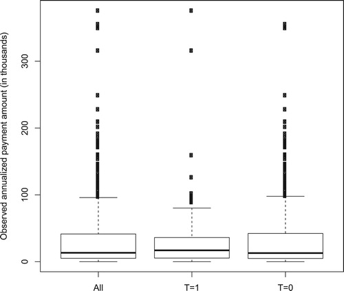
Two issues with this dataset actually motivated our study. First, the distribution of annualised payment is right-skewed as shown by the box plots in Figure 1 for all patients and two groups. The overall median, mean, 75% quantile, and maximum of observed payment are about 13, 31, 41, and 376 thousand dollars, respectively. This suggests the need for estimating quantile treatment effects. Second, the dataset consists of three discrete and ninety-four continuous covariates including medicare status, baseline payments, as well as other baseline characteristics of patients. Thus, dimension reduction is needed in nonparametric kernel estimation.

Figure 1. Boxplots of observed annualised payment amount (in thousands) for overall, CCM group T = 1, and non-CCM group T = 0.

For sufficient dimension reduction, we adopt the semiparametric directional regression method proposed by Ma and Zhu (2012). After sufficient dimension reduction, $S_T$ has 7 dimensions, $S_{Y_0}$ has 5 dimensions, $S_{Y_1}$ has 8 dimensions, and $S_{Y_0,Y_1}$ has 13 dimensions.

Results for three choices of $(S_0,S_1)$ considered in simulation are shown in Table 3 for estimating ATE and QTE with $\tau =25\mathrm{\%}$, 50%, and 75%. Standard errors (SE) for all estimates are calculated using the bootstrap with 200 replications.

Table 3. Estimates and standard errors (SE) for the University of Wisconsin Health ACO data.

		IPW		REG		AIPW
	$S_0,S_1$	Estimate	SE	Estimate	SE	Estimate	SE
25% QTE	$S_T$	0.16	1.00	0.52	1.10	0.39	1.15
	$S_{Y_0,Y_1}$	0.47	0.91	0.57	0.84	0.47	0.89
	$S_{Y_0}$,$S_{Y_1}$	0.47	0.92	−0.10	0.81	0.47	0.88
50% QTE	$S_T$	2.82	2.67	1.59	2.76	3.31	2.64
	$S_{Y_0,Y_1}$	3.21	2.52	2.34	2.63	3.27	2.46
	$S_{Y_0},S_{Y_1}$	3.27	2.41	3.57	2.42	3.27	2.37
75% QTE	$S_T$	−6.09	4.74	−5.31	4.65	−6.33	4.62
	$S_{Y_0,Y_1}$	−8.51	3.92	−5.14	3.90	−8.38	3.82
	$S_{Y_0},S_{Y_1}$	−8.38	3.83	−8.65	3.72	−8.14	3.76
ATE	$S_T$	−2.36	3.72	−2.54	3.83	−2.11	3.53
	$S_{Y_0,Y_1},S_{Y_0,Y_1}$	−5.68	3.09	−3.41	2.93	−6.03	3.05
	$S_{Y_0},S_{Y_1}$	−5.42	2.93	−5.89	2.78	−5.24	2.87

SE: standard error by bootstrapping

From Table 3, the 25% and 50% QTEs are not significant by all methods. When $S_{Y_k}$ or $S_{Y_0,Y_1}$ is used, the 75% QTE is significantly less than 0, and in terms of SE, the estimate using $S_{Y_k}$, k = 0, 1, is more efficient than the estimate using $S_{Y_0,Y_1}$. However, the estimate of 75% QTE using $S_T$ is inefficient due to the large variation of using $S_T$ so that the result is insignificant.

Since 75% QTE is significantly negative, the result indicates that receiving CCM intervention effectively helps reducing medical payment for the high-cost patients. But CCM intervention is not so useful for the low-cost or median-cost patients, as 25% and 50% QTEs are not significant. These results may be useful for decision making in ACO.

For comparison, we also include estimates of ATE and SE. The results in the last block of Table 3 show that ATE is not significant by all methods. It is interesting to see that estimates of ATE are all negative whereas estimates of 50% QTE are all positive although they are not significant, which may be caused by fact that the distribution of annualised payment is right-skewed.

The example shows the usefulness of assessing QTEs with different percentages. If we only estimate ATE, no useful conclusion can be made in this example. Even if we check 50% QTE instead of ATE because of the existing skewness, we still cannot obtain any useful conclusion.

Acknowledgments

We are grateful to the editor, the associate editor, and two anonymous referees for their insightful comments and suggestions, which have led to significant improvements.

Disclosure statement

No potential conflict of interest was reported by the authors.

Additional information

Funding

Our research was supported by the National Natural Science Foundation of China (11871287, 11831008), the Natural Science Foundation of Tianjin (18JCYBJC41100), the Fundamental Research Funds for the Central Universities, the Key Laboratory for Medical Data Analysis and Statistical Research of Tianjin, the Chinese 111 Project (B14019), the U.S. National Science Foundation (DMS-1612873 and DMS-1914411). This research was partially supported through a Patient-Centered Outcomes Research Institute (PCORI) Award (ME-1409-21219).

Notes on contributors

Ying Zhang

Ying Zhang is a Ph.D. candidate, Department of Statistics, University of Wisconsin-Madison.

Lei Wang

Dr Lei Wang holds a Ph.D. in statistics from East China Normal University. He is an assistant professor of statistics at Nankai University. His research interests include empirical likelihood and missing data problems.

Menggang Yu

Dr Menggang Yu holds a Ph.D. in biostatistics from the University of Michigan. He is now a professor of biostatistics at the University of Wisconsin-Madison. Besides developing statistical methodology related to cancer research and clinical trials, Dr Yu is also very interested in health services research.

Jun Shao

Dr Jun Shao holds a Ph.D. in statistics from the University of Wisconsin-Madison. He is a professor of statistics at the University of Wisconsin-Madison. His research interests include variable selection and inference with high dimensional data, sample surveys, and missing data problems.

Appendices

Appendix 1. Semiparametric efficiency bound of estimating θ with $S_k$

Throughout the Appendix, the S, $S_k$, $S_{Y_k}$, $S_{Y_0,Y_1}$, $S_T$, $S_{\mathrm{m}\mathrm{i}\mathrm{n}}$ are linear functions of X, i.e. $S=B^{\mathrm{\top }}X$ with B being a $p\times d$ matrix, $S_k=B_k^{\mathrm{\top }}X$ with $B_k$ being a $p\times d_k$ matrix, etc.

Lemma A.1

Assume $T\perp (Y_0,Y_1)|X$ and $Y_k\perp X|S_k$, and the distribution of $Y_k$ has density $f_k$ with $f_k\left(q_{k,\tau }\right)>0$, k = 0, 1. A lower bound for the asymptotic variance of any asymptotically normal estimator of $\theta =q_{1,\tau }-q_{0,\tau }$ is given by (A1) $\begin{array}{rl}{V}_{S_0,S_1}^{\ast }& =\mathrm{v}\mathrm{a}\mathrm{r}\left\{E\left(g_1\right(Y_1\left)|S_1\right)-E\left(g_0\right(Y_0\left)|S_0\right)\right\}\\ & +\sum _{k=0,1}E\left\{\frac{\mathrm{v}\mathrm{a}\mathrm{r}\left(g_k\right(Y_k\left)|S_k\right)}{P(T=k|S_k)}\right\},\end{array}$(A1) where $g_k\left(Y_k\right)=-\left(\mathbf{1}\right\{Y_k\le q_{k,\tau }\}-\tau )/f_k\left(q_{k,\tau }\right)$, k = 0, 1. If $Y_k\perp X|S_k$, $Y_k\perp X|S_k^{\prime }$, and $\mathcal{L}\left(S_k\right)\subseteq \mathcal{L}\left(S_k^{\prime }\right)$, $k=0,1$, then $V_{S_0,S_1}^{\ast }\le V_{S_0^{\prime },S_1^{\prime }}^{\ast }$, where $\mathcal{L}\left(S\right)$ denotes the linear space generated by columns of B for $S=B^{\mathrm{\top }}X$.

Proof

Proof of Lemma A.1

Our derivation of the efficiency bound mimics the proof in Firpo (2007) which is a direct application of the semiparametric efficiency theory from Bickel et al. (1993). Following the proof of Firpo (2007), one may easily see that knowing $T|X=T|S_T$ won't change the semiparametric efficiency bound, which is similar with the ATE case in Hahn (1998). In our proof for Lemma A.1, one only needs to carefully keep $S_1$ and $S_0$ separate in the derivation. The construction of the efficient influence function is more involved algebraically. We only provide a sketch of the proof for the case $S_k=S_{Y_k}$ here. The density of $(Y_0,Y_1,T,X)$ at $(y_0,y_1,k,x)$ is $q(y_0,y_1,k,x)=g(y_0,y_1|x)\pi \left(x{)}^k\right\{1-\pi \left(x\right){\}}^{1-k}f\left(x\right),$ where $g(y_0,y_1|x)$ denotes the conditional distribution of $(Y_0,Y_1)$ given X, $f\left(x\right)$ denotes the marginal distribution of X and $\pi \left(x\right)=P(T=1|X=x)$. The density of $(Z,T,X)$ at $(z,k,x)$ is then equal to $\begin{array}{rl}q(z,k,x)& =\left\{g_1\right(z|x\left)\pi \right(x\left){\}}^k\right\{g_0\left(z|x\right)(1-\pi (x\left)\right){\}}^{1-k}f\left(x\right)\\ & =\left\{h_1\right(z|S_{y_1}\left)\pi \right(x\left){\}}^k\right\{h_0\left(z|S_{y_0}\right)(1-\pi (x\left)\right){\}}^{1-k}f\left(x\right),\end{array}$ where $g_1(\cdot |x)=\int g(y_0,\cdot |x)\mathrm{d}{y}_0$, $g_0(\cdot |x)=\int g(\cdot ,y_1|x)\mathrm{d}{y}_1$. The second equality holds because by the definition of $S_{Y_1},S_{Y_0}$, there exist functions $h_1$ and $h_0$ that $g_1(\cdot |x)=h_1(\cdot |S_{y_1})$ and $g_0(\cdot |x)=h_0(\cdot |S_{y_0})$. For a regular parametric submodel $q(z,k,x)$ with parameter w, $\begin{array}{rl}{q}_{\omega }(z,k,x)& =\left\{h_1\right(z|S_{y_1},\omega \left)\pi \right(x,\omega ){\}}^k\\ & \times \left\{h_0\right(z|S_{y_0},\omega \left)\right(1-\pi (x,\omega )\left){\}}^{1-k}f\right(x,\omega ).\end{array}$ The score function of this parametric submodel is $\begin{array}{rl}s(z,k,x|\omega )& =k{s}_1(z|S_{y_1},\omega )+(1-k)s_0(z|S_{y_0},\omega )\\ & +\frac{\{k-\pi (x,\omega \left)\right\}\frac{\mathrm{\partial }}{\mathrm{\partial }\omega }\pi (x,\omega )}{\pi (x,\omega )\{1-\pi (x,\omega \left)\right\}}+d(x,\omega ),\end{array}$ where $d(x,\omega )={f(x,\omega )}^{-1}\left(\mathrm{\partial }f(x,\omega )/\mathrm{\partial }\omega \right),$ $s_1(z|S_{y_1},\omega )={h_1(z|S_{y_1},\omega )}^{-1}\left(\mathrm{\partial }{h}_1(z|S_{y_1},\omega )/\mathrm{\partial }\omega \right),$ $s_0(z|S_{y_0},\omega )=h_0(z|S_{y_0},\omega {)}^{-1}(\mathrm{\partial }{h}_0(z|S_{y_0},\omega )/\mathrm{\partial }\omega )$. Therefore, the tangent space is equal to $\begin{array}{rl}\mathcal{T}& =\left\{\phantom{\int d\left(x\right)f\left(x\right)\mathrm{d}x=0\mathrm{a}\mathrm{n}\mathrm{d}a\left(x\right)\mathrm{i}\mathrm{s}\mathrm{u}\mathrm{n}\mathrm{r}\mathrm{e}\mathrm{s}\mathrm{t}\mathrm{r}\mathrm{i}\mathrm{c}\mathrm{t}\mathrm{e}\mathrm{d}}k{s}_1\left(z|S_{y_1}\right)+(1-k)s_0\left(z|S_{y_0}\right)\right.\\ & +a\left(x\right)(k-\pi (x\left)\right)+d\left(x\right):\mathrm{w}\mathrm{h}\mathrm{e}\mathrm{r}\mathrm{e}(s_0,s_1,d,a)\phantom{\int }\\ & \mathrm{s}\mathrm{a}\mathrm{t}\mathrm{i}\mathrm{s}\mathrm{f}\mathrm{i}\mathrm{e}\mathrm{s}\int s_j\left(z|S_{y_j}\right)h_j\left(z|S_{y_j}\right)\mathrm{d}y=0,\\ & \times \left.\int d\left(x\right)f\left(x\right)\mathrm{d}x=0\mathrm{a}\mathrm{n}\mathrm{d}a\left(x\right)\mathrm{i}\mathrm{s}\mathrm{u}\mathrm{n}\mathrm{r}\mathrm{e}\mathrm{s}\mathrm{t}\mathrm{r}\mathrm{i}\mathrm{c}\mathrm{t}\mathrm{e}\mathrm{d}\right\}.\end{array}$ For the parametric submodel with parameter ω under consideration, $q_{k,\tau }\left(\omega \right)$, the τ-th quantile for $Y_k$, k = 0, 1, satisfies $0=E_{\omega }\left(\mathbf{1}\right\{Y_k\le q_{k,\tau }\left(\omega \right)\}-\tau )=\int \int \left(\mathbf{1}\right\{z\le q_{k,\tau }\left(\omega \right)\}-\tau )h_k(z|S_{Y_k},\omega )\mathrm{d}zf(x,\omega )\mathrm{d}x$. Let $\theta \left(\omega \right)=q_{1,\tau }\left(\omega \right)-q_{0,\tau }\left(\omega \right)$, and remember $g_k\left(Y_k\right)=-\left(\mathbf{1}\right\{Y_k\le q_{k,\tau }\}-\tau )/f_k\left(q_{k,\tau }\right)$, k = 0, 1. By an application of Leibnitz's rule, $\begin{array}{rl}\frac{\mathrm{\partial }\theta \left(\omega \right)}{\mathrm{\partial }\omega }& =\int \int g_1\left(z\right)s_1(z|S_{y_1},\omega )h_1(z|S_{y_1},\omega )f(x,\omega )\mathrm{d}z\mathrm{d}x\\ & +\int E_{\omega }\left(g_1\left(z\right)-g_0\left(z\right)|X=x\right)\mathrm{d}(x,\omega )f(x,\omega )\mathrm{d}x\\ & -\int \int g_0\left(z\right)s_0(z|S_{y_0},{\omega }_0)h_0\left(z|S_{y_0}\right)f(x,\omega )\mathrm{d}z\mathrm{d}x.\end{array}$ Let $\begin{array}{rl}F(Z,T,X)& =\frac{T\left\{g_1\right(Z)-E(g_1\left(Z\right)|S_{Y_1}\left)\right\}}{P(T=1|S_{Y_1})}\\ & -\frac{(1-T)\left\{g_0\right(Z)-E(g_0\left(Z\right)|S_{Y_0}\left)\right\}}{1-P(T=1|S_{Y_0})}\\ & +E\left(g_1\right(Z)-g_0(Z\left)|X\right),\end{array}$ and the true parameter ω is $\omega ={\omega }_0$, i.e. $\theta =\theta \left({\omega }_0\right)$, then we have (A2) $\begin{array}{rl}& E\left\{F(Z,T,X)s(Z,T,X|{\omega }_0)\right\}\\ & =E\left[\frac{T\left\{g_1\right(Z)-E(g_1\left(Z\right)|S_{Y_1}\left)\right\}}{P(T=1|S_{Y_1})}s(Z,T,X|{\omega }_0)\right]\\ & -E\left[\frac{(1-T)\left\{g_0\right(Z)-E(g_0\left(Z\right)|S_{Y_0}\left)\right\}}{1-P(T=1|S_{Y_0})}s(Z,T,X|{\omega }_0)\right]\\ & +E\left[E\left(g_1\right(Z)-g_0(Z\left)|X\right)s(Z,T,X|{\omega }_0)\right].\end{array}$(A2) For the three terms in (A2(A2) $\begin{array}{rl}& E\left\{F(Z,T,X)s(Z,T,X|{\omega }_0)\right\}\\ & =E\left[\frac{T\left\{g_1\right(Z)-E(g_1\left(Z\right)|S_{Y_1}\left)\right\}}{P(T=1|S_{Y_1})}s(Z,T,X|{\omega }_0)\right]\\ & -E\left[\frac{(1-T)\left\{g_0\right(Z)-E(g_0\left(Z\right)|S_{Y_0}\left)\right\}}{1-P(T=1|S_{Y_0})}s(Z,T,X|{\omega }_0)\right]\\ & +E\left[E\left(g_1\right(Z)-g_0(Z\left)|X\right)s(Z,T,X|{\omega }_0)\right].\end{array}$(A2) ), after some algebra, we have, respectively, $\begin{array}{rl}& E\left[\frac{T\left\{g_1\right(Z)-E(g_1\left(Z\right)|S_{Y_1}\left)\right\}}{P(T=1|S_{Y_1})}s(Z,T,X|{\omega }_0)\right]\\ & =E\left[\right\{g_1\left(Y_1\right)-E\left(g_1\right(Y_1\left)|S_{Y_1}\right)\left\}{s}_1\right(Y_1|S_{Y_1},{\omega }_0\left)\right],\\ & \times E\left[\frac{(1-T)\left\{g_0\right(Z)-E(g_0\left(Z\right)|S_{Y_0}\left)\right\}}{1-P(T=1|S_{Y_0})}s(Z,T,X|{\omega }_0)\right]\\ & =E\left[\right\{g_0\left(Z\right)-E\left(g_0\right(Z\left)|S_{Y_0}\right)\left\}{s}_0\right(Y_0|S_{Y_0},{\omega }_0\left)\right],\\ & \times E\left[\right\{E\left(g_1\right(Z)-g_0(Z\left)|X\right)\left\}s\right(Z,T,X|{\omega }_0\left)\right]\\ & =E\left\{E\right(g_1\left(Y_1\right)-g_0\left(Y_0\right)|X\left)d\right(X,{\omega }_0\left)\right\}.\end{array}$ Therefore, $E\left\{F\right(Z,T,X\left)s\right(Z,T,X|{\omega }_0\left)\right\}=\mathrm{\partial }\theta \left({\omega }_0\right)/\mathrm{\partial }\omega .$ The efficiency bound is the expected square of the projection of F on $\mathcal{T}$. Because $F\in \mathcal{T}$, the projection of F on $\mathcal{T}$ is itself. The conclusion follows.

For the second part of Lemma A.1, suppose $S_0$, $S_1$ satisfy $\mathcal{L}\left(S_0\right)\supseteq \mathcal{L}\left(S_{Y_0}\right)$, $\mathcal{L}\left(S_1\right)\supseteq \mathcal{L}\left(S_{Y_1}\right)$. Since $\begin{array}{rl}{V}_{S_{Y_1},S_{Y_0}}^{\ast }& =\mathrm{V}\mathrm{a}\mathrm{r}\left\{E\right(g_1\left(Y_1\right)|X)-E(g_0\left(Y_0\right)|X\left)\right\}\\ & +E\left\{\frac{\mathrm{V}\mathrm{a}\mathrm{r}\left(g_1\right(Y_1\left)|X\right)}{P(T=1|S_{Y_1})}\right\}+E\left\{\frac{\mathrm{V}\mathrm{a}\mathrm{r}\left(g_0\right(Y_0\left)|X\right)}{P(T=0|S_{Y_0})}\right\},\\ V_{S_1,S_0}^{\ast }& =\mathrm{V}\mathrm{a}\mathrm{r}\left\{E\right(g_1\left(Y_1\right)|X)-E(g_0\left(Y_0\right)|X\left)\right\}\\ & +E\left\{\frac{\mathrm{V}\mathrm{a}\mathrm{r}\left(g_1\right(Y_1\left)|X\right)}{P(T=1|S_1)}\right\}+E\left\{\frac{\mathrm{V}\mathrm{a}\mathrm{r}\left(g_0\right(Y_0\left)|X\right)}{P(T=0|S_0)}\right\}.\end{array}$ We only need to prove $E\left\{\frac{\mathrm{V}\mathrm{a}\mathrm{r}\left(g_1\right(Y_1\left)|X\right)}{P(T=1|S_{Y_1})}\right\}\le E\left\{\frac{\mathrm{V}\mathrm{a}\mathrm{r}\left(g_1\right(Y_1\left)|X\right)}{P(T=1|S_1)}\right\}.$ By Jensen's inequity, we have $\frac{1}{E\left\{E\right(T|S_1\left)|S_{Y_1}\right\}}\le E\left\{\left.\frac{1}{E\left(T|S_1\right)}\right|S_{Y_1}\right\}.$ Thus the conclusion follows from the inequality below. $\begin{array}{rl}E\left[\frac{\mathrm{V}\mathrm{a}\mathrm{r}\left(g_1\right(Y_1\left)|X\right)}{P(T=1|S_{Y_1})}\right]& =E\left[\frac{\mathrm{V}\mathrm{a}\mathrm{r}\left(g_1\right(Y_1\left)|X\right)}{E\left\{E\right(T|S_1\left)|S_{Y_1}\right\}}\right]\\ & \le E\left[\mathrm{V}\mathrm{a}\mathrm{r}\left(g_1\right(Y_1\left)|X\right)E\left\{\left.\frac{1}{E\left(T|S_1\right)}\right|S_{Y_1}\right\}\right]\\ & =E\left[E\left\{\left.\frac{\mathrm{V}\mathrm{a}\mathrm{r}\left(g_1\right(Y_1\left)|X\right)}{E\left(T|S_1\right)}\right|S_{Y_1}\right\}\right]\\ & =E\left\{\frac{\mathrm{V}\mathrm{a}\mathrm{r}\left(g_1\right(Y_1\left)|X\right)}{P(T=1|S_1)}\right\}.\end{array}$

Appendix 2

Conditions for Theorem 2.1

(C1)	$Y_k$ is a continuous random variable and for any fixed $\tau \in (0,1)$ there exists a unique $q_{k,\tau }$ that $P(Y_k\le q_{k,\tau })=\tau$ for k = 0, 1.
(C2)	${\pi }_k\left(S_k\right)$ is bounded away from 0 and 1.
(C3)	$S_k$ has compact support for k = 0, 1.
(C4)	The function ${\pi }_k\left(S_k\right)$, the density function $f\left(S_k\right)$ and $E\left(\mathbf{1}\right\{Y_k\le q_{k,\tau }\left\}|S_k\right)$ all have bounded partial derivatives with respect to $S_k$ up to $r_k$ order, $f\left(S_k\right){\pi }_k\left(S_k\right)$ is bounded away from 0.
(C5)	The kernel ${\mathcal{K}}_k$ is bounded up to second order derivative.
(C6)	The smoothing bandwidth $h_{kn}$ satisfies $n{h}_{kn}^2\to \mathrm{\infty }$, $n{h}_{kn}^{d_k}\to \mathrm{\infty }$ and $\sqrt{n}{h}_{kn}^{r_k}\to 0$ as $n\to \mathrm{\infty }$. Here $r_k$ is the order of the kernel ${\mathcal{K}}_k$.

Appendix 3

Proof of Theorem 2.1

Proof

Proof of Theorem 2.1

(i) In the case that $S_k=X$, Firpo (2007) proved the asymptotics of ${\hat{\theta }}_{\mathrm{I}\mathrm{P}\mathrm{W}}$ using kernel method, Chen et al. (2015) proved the asymptotics of ${\hat{\theta }}_{\mathrm{R}\mathrm{E}\mathrm{G}}$ using kernel method. Following the proofs in their papers and substituting X by $S_k$, $\sqrt{n}\left(\hat{\theta }\right(S_0,S_1)-\theta )$ is asymptotically equivalent to (A3) $\begin{array}{rl}& \frac{1}{\sqrt{n}}\sum _{i=1}^n\left[\frac{T_i{g}_1\left(Z_i\right)}{{\pi }_1\left(S_{1i}\right)}-\frac{E\left(g_1\left(Y_1\right)|S_{1i}\right)\{T_i-{\pi }_1(S_{1i}\left)\right\}}{{\pi }_1\left(S_{1i}\right)}\right]\\ & -\frac{1}{\sqrt{n}}\sum _{i=1}^n\left[\frac{(1-T_i)g_0\left(Z_i\right)}{{\pi }_0\left(S_{0i}\right)}\right.\\ & \left.-\frac{E\left(g_0\left(Y_0\right)|S_{0i}\right)\left\{\right(1-T_i)-{\pi }_0(S_{0i}\left)\right\}}{{\pi }_{0i}\left(S_{0i}\right)}\right]+o_p\left(1\right),\end{array}$(A3) where $S_{ki}$ is the ith observation of $S_k$, ${\pi }_k\left(S_{ki}\right)=P(T=k|S_k=S_{ki})$ for k = 0, 1. By direct but tedious calculation, the covariance of the two summation terms in (A3(A3) $\begin{array}{rl}& \frac{1}{\sqrt{n}}\sum _{i=1}^n\left[\frac{T_i{g}_1\left(Z_i\right)}{{\pi }_1\left(S_{1i}\right)}-\frac{E\left(g_1\left(Y_1\right)|S_{1i}\right)\{T_i-{\pi }_1(S_{1i}\left)\right\}}{{\pi }_1\left(S_{1i}\right)}\right]\\ & -\frac{1}{\sqrt{n}}\sum _{i=1}^n\left[\frac{(1-T_i)g_0\left(Z_i\right)}{{\pi }_0\left(S_{0i}\right)}\right.\\ & \left.-\frac{E\left(g_0\left(Y_0\right)|S_{0i}\right)\left\{\right(1-T_i)-{\pi }_0(S_{0i}\left)\right\}}{{\pi }_{0i}\left(S_{0i}\right)}\right]+o_p\left(1\right),\end{array}$(A3) ) is $-E\left(g_0\right(Y_0\left)\right)E\left(g_1\right(Y_1\left)\right)+E\left\{E\right(g_0\left(Y_0\right)|S_0\left)E\right(g_1\left(Y_1\right)|S_1\left)\right\}$. Their corresponding variances are $\begin{array}{rl}& \mathrm{V}\mathrm{a}\mathrm{r}\left[\frac{T{g}_1\left(Z\right)}{{\pi }_1\left(S_1\right)}-\frac{E\left(g_1\right(Y_1\left)|S_1\right)}{{\pi }_1\left(S_1\right)}\{T-{\pi }_1(S_1\left)\right\}\right]\\ & =\mathrm{V}\mathrm{a}\mathrm{r}\left\{E\left(g_1\left(Y_1\right)|S_1\right)\right\}+E\left\{\frac{\mathrm{V}\mathrm{a}\mathrm{r}\left(g_1\right(Y_1\left)|S_1\right)}{{\pi }_1\left(S_1\right)}\right\},\\ & \mathrm{V}\mathrm{a}\mathrm{r}\left[\frac{(1-T)g_0\left(Y_0\right)}{{\pi }_0\left(S_0\right)}-\frac{E\left(g_0\right(Y_0\left)|S_0\right)}{{\pi }_0\left(S_0\right)}\left\{\right(1-T)-{\pi }_0(S_0\left)\right\}\right]\\ & =\mathrm{V}\mathrm{a}\mathrm{r}\left\{E\left(g_0\left(Y_0\right)|S_0\right)\right\}+E\left\{\frac{\mathrm{V}\mathrm{a}\mathrm{r}\left(g_0\right(Y_0\left)|S_0\right)}{{\pi }_0\left(S_0\right)}\right\}.\end{array}$ Thus the asymptotic variance of $\hat{\theta }(S_0,S_1)$ is $\begin{array}{rl}& \mathrm{V}\mathrm{a}\mathrm{r}\left\{E\left(g_1\left(Y_1\right)|S_1\right)-E\left(g_0\left(Y_0\right)|S_0\right)\right\}\\ & +E\left\{\frac{\mathrm{V}\mathrm{a}\mathrm{r}\left(g_1\right(Y_1\left)|S_1\right)}{{\pi }_1\left(S_1\right)}\right\}+E\left\{\frac{\mathrm{V}\mathrm{a}\mathrm{r}\left(g_0\right(Y_0\left)|S_0\right)}{{\pi }_0\left(S_0\right)}\right\}.\end{array}$ (ii) Here we only list the proof for regression type estimator ${\hat{\theta }}_{\mathrm{R}\mathrm{E}\mathrm{G}}$ with $d_0=d_1=1$. We only derive the difference of ${\hat{q}}_{1,\tau }$ between using true $B_k$ and estimated $B_k$ for regression estimator, the proof for the ${\hat{q}}_{0,\tau }$ is similar. For simplicity, we denote $S_1$, $B_1$, $h_{1n}$, ${\mathcal{K}}_1$, $g_1(\cdot )$, ${\pi }_1(\cdot )$ as S, B, h, $\mathcal{K}$, $g(\cdot )$, $\pi (\cdot )$ respectively and define ${\mathcal{K}}_h(\cdot )=h^{-1}\mathcal{K}(\cdot /h)$ in the following proof. Let ${\mathrm{\Delta }}_{ij}={\mathcal{K}}_h({\hat{B}}^{\mathrm{\top }}{X}_j-{\hat{B}}^{\mathrm{\top }}{X}_i)-{\mathcal{K}}_h(B^{\mathrm{\top }}{X}_j-B^{\mathrm{\top }}{X}_i)$, it can be verified that $\begin{array}{rl}& \frac{1}{n}\sum _{i=1}^n\left\{\frac{\sum _{j=1}^n{T}_{j}g\left(Z_j\right){\mathcal{K}}_h({\hat{B}}^{\mathrm{\top }}{X}_j-{\hat{B}}^{\mathrm{\top }}{X}_i)}{\sum _{j=1}^n{T}_j{\mathcal{K}}_h({\hat{B}}^{\mathrm{\top }}{X}_j-{\hat{B}}^{\mathrm{\top }}{X}_i)}\right.\\ & -\left.\frac{\sum _{j=1}^n{T}_{j}g\left(Z_j\right){\mathcal{K}}_h(B^{\mathrm{\top }}{X}_j-B^{\mathrm{\top }}{X}_i)}{\sum _{j=1}^n{T}_j{\mathcal{K}}_h(B^{\mathrm{\top }}{X}_j-B^{\mathrm{\top }}{X}_i)}\right\}\\ & =\frac{1}{n}\sum _{i=1}^n\left\{\frac{\sum _{j=1}^n{T}_{j}g\left(Z_j\right){\mathcal{K}}_h(S_j-S_i)+\sum _{j=1}^n{T}_{j}g\left(Z_j\right){\mathrm{\Delta }}_{ij}}{\sum _{j=1}^n{T}_j{\mathcal{K}}_h(S_j-S_i)+\sum _{j=1}^n{T}_j{\mathrm{\Delta }}_{ij}}\right.\\ & -\left.\frac{\sum _{j=1}^n{T}_{j}g\left(Z_j\right){\mathcal{K}}_h(S_j-S_i)}{\sum _{j=1}^n{T}_j{\mathcal{K}}_h(S_j-S_i)}\right\}\\ & \equiv A_1+A_2+A_3,\end{array}$ where $\begin{array}{rl}{A}_1& =\frac{1}{n^2}\sum _{i=1}^n\sum _{j=1}^n\left\{\frac{T_{j}g\left(Z_j\right){\mathrm{\Delta }}_{ij}}{\pi \left(S_i\right)f\left(S_i\right)}-\frac{T_{j}E\left(g\right(Z_i\left)|S_i\right){\mathrm{\Delta }}_{ij}}{\pi \left(S_i\right)f\left(S_i\right)}\right\},\\ A_2& =-\frac{1}{n^2}\sum _{i=1}^n\sum _{j=1}^n\left\{\phantom{\frac{T_{j}g\left(Z_j\right){\mathrm{\Delta }}_{ij}}{\frac{1}{n}\sum _{l=1}^n{T}_l{\mathcal{K}}_h(S_l-S_i)+\frac{1}{n}\sum _{l=1}^n{T}_l{\mathrm{\Delta }}_{il}}}\frac{T_{j}g\left(Z_j\right){\mathrm{\Delta }}_{ij}}{\pi \left(S_i\right)f\left(S_i\right)}\right.\\ & -\left.\frac{T_{j}g\left(Z_j\right){\mathrm{\Delta }}_{ij}}{\frac{1}{n}\sum _{l=1}^n{T}_l{\mathcal{K}}_h(S_l-S_i)+\frac{1}{n}\sum _{l=1}^n{T}_l{\mathrm{\Delta }}_{il}}\right\},\\ A_3& =\frac{1}{n^2}\sum _{i=1}^n\sum _{j=1}^n{T}_j{\mathrm{\Delta }}_{ij}\left\{\phantom{\frac{E\left(g\right(Z_i\left)|S_i\right)-\frac{\sum _{l=1}^n{T}_{l}g\left(Z_l\right){\mathcal{K}}_h(S_l-S_i)}{\sum _{l=1}^n{T}_l{\mathcal{K}}_h(S_l-S_i)}}{\frac{1}{n}\sum _{l=1}^n{T}_l{\mathcal{K}}_h(S_l-S_i)+\frac{1}{n}\sum _{l=1}^n{T}_l{\mathrm{\Delta }}_{il}}}\frac{E\left(g\right(Z_i\left)|S_i\right)}{\pi \left(S_i\right)f\left(S_i\right)}\right.\\ & -\frac{E\left(g\right(Z_i\left)|S_i\right)}{\frac{1}{n}\sum _{l=1}^n{T}_l{\mathcal{K}}_h(S_l-S_i)+\frac{1}{n}\sum _{l=1}^n{T}_l{\mathrm{\Delta }}_{il}}\phantom{\frac{E\left(g\right(Z_i\left)|S_i\right)-\frac{\sum _{l=1}^n{T}_{l}g\left(Z_l\right){\mathcal{K}}_h(S_l-S_i)}{\sum _{l=1}^n{T}_l{\mathcal{K}}_h(S_l-S_i)}}{\frac{1}{n}\sum _{l=1}^n{T}_l{\mathcal{K}}_h(S_l-S_i)+\frac{1}{n}\sum _{l=1}^n{T}_l{\mathrm{\Delta }}_{il}}}\\ & \left.+\frac{E\left(g\right(Z_i\left)|S_i\right)-\frac{\sum _{l=1}^n{T}_{l}g\left(Z_l\right){\mathcal{K}}_h(S_l-S_i)}{\sum _{l=1}^n{T}_l{\mathcal{K}}_h(S_l-S_i)}}{\frac{1}{n}\sum _{l=1}^n{T}_l{\mathcal{K}}_h(S_l-S_i)+\frac{1}{n}\sum _{l=1}^n{T}_l{\mathrm{\Delta }}_{il}}\right\}.\end{array}$ Since ${\mathrm{\Delta }}_{ij}={\mathcal{K}}_h({\hat{B}}^{\mathrm{\top }}{X}_j-{\hat{B}}^{\mathrm{\top }}{X}_i)-{\mathcal{K}}_h(B^{\mathrm{\top }}{X}_j-B^{\mathrm{\top }}{X}_i)$, using a Taylor expansion around $B^{\mathrm{\top }}{X}_j-B^{\mathrm{\top }}{X}_i$ for ${\mathrm{\Delta }}_{ij}$ and plugging in $A_1$, we have $\begin{array}{rl}{A}_1& =\frac{(\hat{B}-B{)}^{\mathrm{\top }}}{n^2}\sum _{i=1}^n\sum _{j=1}^n\left\{\frac{T_j\left\{g\right(Z_j)-E(g\left(Z_i\right)|S_i\left)\right\}}{\pi \left(S_i\right)f\left(S_i\right)}\right.\\ & \times \left.\frac{1}{h}\left[{\mathcal{K}}^{\prime }\left(\frac{B^{\mathrm{\top }}{X}_j-B^{\mathrm{\top }}{X}_i}{h}\right)\frac{X_j-X_i}{h}\right]\right\}+o_p\left(n^{-1/2}\right)\\ & \equiv \frac{(\hat{B}-B{)}^{\mathrm{\top }}}{n^2}\sum _{i=1}^n\sum _{j=1}^n{Q}_{ij}+o_p\left(n^{-1/2}\right).\end{array}$ Denote $A_{11}=\sum _{i=1}^n\sum _{j=1}^n{Q}_{ij}/n^2$ and ${\breve{A}}_{11}=\sum _{i=1}^n\sum _{j=1}^{n}E(Q_{ij}|X_i,g(Z_i),T_i)/n^2$. Note $\begin{array}{rl}& E\left\{\left.\frac{1}{h}{T}_j{\mathcal{K}}^{\prime }\left(\frac{S_j-S_i}{h}\right)\left(\frac{X_j-X_i}{h}\right)\right|(X_i,Z_i,T_i)=(x_i,z_i,t_i)\right\}\\ & =E\left[E\left\{\left.\frac{1}{h}{T}_j{\mathcal{K}}^{\prime }\left(\frac{S_j-s_i}{h}\right)\frac{X_j-x_i}{h}\right|S_j\right\}\right]\\ & =E\left[\frac{1}{h^2}{\mathcal{K}}^{\prime }\left(\frac{S_j-s_i}{h}\right)E\left\{T_j\right(X_j-x_i\left)|S_j\right\}\right]\\ & ={\left.-\frac{\mathrm{\partial }\left[E\right\{T(X-x_i)|S=t\left\}f\right(t\left)\right]}{\mathrm{\partial }t}\right|}_{t=s_i}+o_p\left(1\right)\\ & =-E(TX|S=s_i)f^{\prime }\left(s_i\right)-x_i\pi \left(s_i\right)f^{\prime }\left(s_i\right)-x_i{\pi }^{\prime }\left(s_i\right)f\left(s_i\right)\\ & +{\left.\frac{\mathrm{\partial }\left\{E\right(TX|S=t\left)\right\}}{\mathrm{\partial }t}\right|}_{t=s_i}f\left(s_i\right)+o_p\left(1\right),\end{array}$ and $\begin{array}{rl}& E\left\{\left.\frac{1}{h}{T}_{j}g\left(Z_j\right){\mathcal{K}}^{\prime }\left(\frac{S_j-s_i}{h}\right)\left(\frac{X_j-x_i}{h}\right)\right|(X_i,Z_i,T_i)=(x_i,z_i,t_i)\right\}\\ & =E\left[E\left\{\left.\frac{1}{h}{T}_{j}g\left(Z_j\right){\mathcal{K}}^{\prime }\left(\frac{S_j-s_i}{h}\right)\frac{X_j-x_i}{h}\right|S_j\right\}\right]\\ & =E\left[\frac{1}{h^2}{\mathcal{K}}^{\prime }\left(\frac{S_j-s_i}{h}\right)E\left\{T_{j}g\right(Z_j\left)\right(X_j-x_i\left)|S_j\right\}\right]\\ & ={\left.-\frac{\mathrm{\partial }\left\{E\left(Tg\left(Z\right)(X-x_i)|S=t\right)f\right(t\left)\right\}}{\mathrm{\partial }t}\right|}_{t=s_i}+o\left(1\right)\\ & =-E\left(Tg\right(Z\left)X|S=s_i\right)f^{\prime }\left(s_i\right)-x_i\pi \left(s_i\right)E\left(g\right(Z)|S=s_i)f^{\prime }\left(s_i\right)\\ & +{\left.\frac{\mathrm{\partial }E\left(Tg\right(Z)X|S=t)}{\mathrm{\partial }t}\right|}_{t=s_i}f\left(s_i\right)\\ & -x_i{\pi }^{\prime }\left(s_i\right)E\left(g\right(Z)|S=s_i)f\left(s_i\right)-x_i\pi \left(s_i\right)\\ & \times \left\{\frac{\mathrm{\partial }E\left(g\right(Z)|S=s_i)}{\mathrm{\partial }S}\right\}f\left(s_i\right)+o_p\left(1\right).\end{array}$ Therefore, $\begin{array}{rl}{\breve{A}}_{11}& =\frac{1}{n}\sum _{i=1}^n\left\{\mathrm{c}\mathrm{o}\mathrm{v}(TX,g(Z)|S=s_i)f^{\prime }\left(s_i\right)\right.\\ & +{\left.\frac{\mathrm{\partial }E\left(Tg\right(Z)X|S=t)}{\mathrm{\partial }t}\right|}_{t=s_i}f\left(s_i\right)\\ & {\left.-\frac{\mathrm{\partial }E(TX|S=t)}{\mathrm{\partial }t}\right|}_{t=s_i}E\left(g\right(Z)|S=s_i)f\left(s_i\right)\\ & -\left.x_i\pi \left(s_i\right)\frac{\mathrm{\partial }E\left(g\right(Z)|S=s_i)}{\mathrm{\partial }S}f\left(s_i\right)\right\}+o_p\left(1\right)\\ & =-\frac{1}{n}\sum _{i=1}^n\left\{\mathrm{c}\mathrm{o}\mathrm{v}(TX,g(Z)|S=s_i)f^{\prime }\left(s_i\right)\right.\\ & +{\left.\frac{\mathrm{\partial }\mathrm{c}\mathrm{o}\mathrm{v}(TX,g(Z)|S=t)}{\mathrm{\partial }t}\right|}_{t=s_i}f\left(s_i\right)\\ & \phantom{{\left.\frac{\mathrm{\partial }\mathrm{c}\mathrm{o}\mathrm{v}(TX,g(Z)|S=t)}{\mathrm{\partial }t}\right|}_{t=s_i}}+E(TX|S=s_i)\frac{\mathrm{\partial }E\left(g\right(Z)|S=s_i)}{\mathrm{\partial }S}f\left(s_i\right)\\ & -\left.x_i\pi \left(s_i\right)\frac{\mathrm{\partial }E\left(g\right(Z)|S=s_i)}{\mathrm{\partial }S}f\left(s_i\right)\right\}+o_p\left(1\right)\\ & =(c_1{)}_{p\times 1}+o_p(1),\end{array}$ where $\begin{array}{rl}{c}_1& =-E\left\{\frac{\mathrm{c}\mathrm{o}\mathrm{v}(TX,g(Z\left)|S\right)f^{\prime }\left(S\right)+\frac{\mathrm{\partial }\mathrm{c}\mathrm{o}\mathrm{v}(TX,g(Z\left)|S\right)}{\mathrm{\partial }S}f\left(S\right)}{\pi \left(S\right)f\left(S\right)}\right\}\\ & +E\left[\frac{\left\{E\right(TX|S)-X\pi (S\left)\right\}\frac{\mathrm{\partial }E\left(g\right(Z\left)|S\right)}{\mathrm{\partial }S}}{\pi \left(S\right)}\right]\\ & =E\left[\frac{\mathrm{\partial }\left\{\pi \right(S{)}^{-1}\}}{\mathrm{\partial }S}\mathrm{c}\mathrm{o}\mathrm{v}(TX,g(Z\left)|S\right)\right.\\ & -\left.\frac{\mathrm{c}\mathrm{o}\mathrm{v}(X,T|S)}{\pi \left(S\right)}\frac{\mathrm{\partial }E\left(g\right(Z\left)|S\right)}{\mathrm{\partial }S}\right].\end{array}$ It can be seen that the first term in $c_1$ will equal to 0 if $Y_1\perp X|S$, while the second term in $c_1$ will equal to 0 if $T\perp X|S$. Thus when both $Y_1\perp X|S$ and $T\perp X|S$ hold, we will have $c_1=0$. Let $A_{11j}=\left(1/n\right)\sum _{i=1}^n{Q}_{ij},{\breve{A}}_{11j}=\left(1/n\right)\sum _{i=1}^{n}E(Q_{ij}|X_i,g(Z_i),T_i))$, we have $\begin{array}{rl}E(A_{11}-{\breve{A}}_{11}{)}^2& =\frac{1}{n^2}\sum _{j=1}^{n}E(A_{11j}-{\breve{A}}_{11j}{)}^2+\frac{2}{n(n-1)}\\ & \times \sum _{j\ne k}E(A_{11j}-{\breve{A}}_{11j})E(A_{11k}-{\breve{A}}_{11k})\\ & =\frac{1}{n}E(A_{11j}-{\breve{A}}_{11j}{)}^2=\frac{1}{n}\{E\left(A_{11j}^2\right)-E\left({\breve{A}}_{11j}^2\right)\}\\ & \le \frac{1}{n}E\left(A_{11j}^2\right)=o_p\left(1\right).\end{array}$ Thus we have $A_{11}=c_1+o_p\left(1\right)$, which leads to $\sqrt{n}{A}_1=c_1^{\mathrm{\top }}\left\{\sqrt{n}\right(\hat{B}-B\left)\right\}+o_p\left(1\right).$ For $A_2$, we also use a Taylor expansion for ${\mathrm{\Delta }}_{ij}$: $\begin{array}{rl}{A}_2& \equiv -\frac{1}{n^2}\sum _{i=1}^n\sum _{j=1}^n\times \left\{\frac{T_{j}g\left(Z_j\right){\mathrm{\Delta }}_{ij}}{\pi \left(S_i\right)f\left(S_i\right)}\right.\\ & -\left.\frac{T_{j}g\left(Z_j\right){\mathrm{\Delta }}_{ij}}{\frac{1}{n}\sum _{l=1}^n{T}_l{\mathcal{K}}_h(S_l-S_i)+\frac{1}{n}\sum _{l=1}^n{T}_l{\mathrm{\Delta }}_{il}}\right\}\\ & =-\frac{1}{n^2}\sum _{i=1}^n\sum _{j=1}^n\\ & \times \left[\frac{T_{j}g\left(Z_j\right)}{h}{\mathcal{K}}^{\prime }\left(\frac{B^{\mathrm{\top }}{X}_j-B^{\mathrm{\top }}{X}_i}{h}\right)(\hat{B}-B{)}^{\mathrm{\top }}\right.\\ & \times \left(\frac{X_j-X_i}{h}\right)\left\{\frac{1}{\pi \left(S_i\right)f\left(S_i\right)}\right.\\ & \left.\left.-\frac{1}{\begin{array}{c}\frac{1}{n}\sum _{l=1}^n{T}_l{\mathcal{K}}_h(S_l-S_i)\\ +\frac{1}{n}\sum _{l=1}^n{T}_l{\mathrm{\Delta }}_{il}\end{array}}\right\}\right]+o_p\left(n^{-1/2}\right).\end{array}$ We then decompose $A_2$ by conditioning on index i, j, that is we define $\begin{array}{rl}{\breve{A}}_2& =-\frac{1}{n^2}\sum _{i=1}^n\sum _{j=1}^n\\ & \times \left[\frac{T_{j}g\left(Z_j\right)}{h}{\mathcal{K}}^{\prime }\left(\frac{B^{\mathrm{\top }}{X}_j-B^{\mathrm{\top }}{X}_i}{h}\right)(\hat{B}-B{)}^{\mathrm{\top }}\left(\frac{X_j-X_i}{h}\right)\right.\\ & \times E\left\{\frac{1}{\pi \left(S_i\right)f\left(S_i\right)}\right.\\ & -\left.\left.\left.\frac{1}{\begin{array}{c}\frac{1}{n}\sum _{l=1}^n{T}_l{\mathcal{K}}_h(S_l-S_i)\\ +\frac{1}{n}\sum _{l=1}^n{T}_l{\mathrm{\Delta }}_{il}\end{array}}\right|X_i,g\left(Z_i\right),T_i\right\}\right].\end{array}$ Since $\begin{array}{rl}& E\left\{\frac{1}{n}\sum _{l=1}^n{T}_l{\mathcal{K}}_h(S_l-S_i)|S_i\right\}\\ & =\pi \left(S_i\right)f\left(S_i\right)+o_p\left(1\right),\\ & E\left\{\frac{1}{n}\sum _{l=1}^n{T}_{l}g\left(Z_l\right){\mathcal{K}}_h(S_l-S_i)|S_i\right\}\\ & =\pi \left(S_i\right)E\left(g\right(Z_i\left)|S_i\right)f\left(S_i\right)+o_p\left(1\right),\end{array}$ using a similar decomposition method as $A_1$, we can also show $\sqrt{n}{A}_2⟹p0$ and $\sqrt{n}{A}_3⟹p0$. Thus we proved that $\begin{array}{rl}& \frac{1}{n}\sum _{i=1}^n\hat{E}\left[g\left(Y_{1i}\right)|{\hat{S}}_i\right]-\frac{1}{n}\sum _{i=1}^n\hat{E}\left[g\left(Y_{1i}\right)|S_i\right]\\ & =\frac{1}{n}\sum _{i=1}^n\left\{\frac{\sum _{j=1}^n{T}_{j}g\left(Z_j\right){\mathcal{K}}_h({\hat{S}}_j-{\hat{S}}_i)}{\sum _{j=1}^n{T}_j{\mathcal{K}}_h({\hat{S}}_j-{\hat{S}}_i)}\right.\\ & -\left.\frac{\sum _{j=1}^n{T}_{j}g\left(Z_j\right){\mathcal{K}}_h(S_j-S_i)}{\sum _{j=1}^n{T}_j{\mathcal{K}}_h(S_j-S_i)}\right\}\\ & =c_1^{\mathrm{\top }}(\hat{B}-B)+o_p\left(1/\sqrt{n}\right).\end{array}$ Note that the REG estimator for $q_{1,\tau }$ based on estimated S is: $\begin{array}{rl}{\hat{q}}_{1,\tau }& =\mathrm{a}\mathrm{r}\mathrm{g}\mathrm{m}\mathrm{i}\mathrm{n}\frac{1}{n}\sum _{i=1}^n\hat{E}\left\{(Y_{1i}-t)(\tau -\mathbf{1}\{Y_{1i}\le t\left\}\right)|\widehat{S_i}\right\}\\ & =\mathrm{a}\mathrm{r}\mathrm{g}\mathrm{m}\mathrm{i}\mathrm{n}\sum _{i=1}^n\left(\hat{E}\left[\left(\mathbf{1}\right\{Y_{1i}\le q_{1,\tau }\}-\tau )(t-q_{1,\tau })|{\hat{S}}_i\right]\right.\\ & \left.+\hat{E}\left[(Y_{1i}-t)\left(\mathbf{1}\right\{Y_{1i}\le q_{1,\tau }\}-\mathbf{1}\{Y_{1i}\le t\left\}\right)|{\hat{S}}_i\right]\right).\end{array}$ Let $u=\sqrt{n}(t-q_{1,\tau })$, $\hat{u}=\sqrt{n}({\hat{q}}_{1,\tau }-q_{1,\tau })$, the optimisation will change to $\begin{array}{rl}\hat{u}& =\mathrm{a}\mathrm{r}\mathrm{g}\mathrm{m}\mathrm{i}\mathrm{n}\left\{\sum _{i=1}^n\frac{u}{\sqrt{n}}\hat{E}\left[\left(\mathbf{1}\right\{Y_{1i}\le q_{1,\tau }\}-\tau )|{\hat{S}}_i\right]\right.\\ & +\sum _{i=1}^n\hat{E}\left[(Y_{1i}-(q_{1,\tau }+u/\sqrt{n}\left)\right)\left(\mathbf{1}\right\{Y_{1i}\le q_{1,\tau }\}\right.\\ & -\left.\left.\mathbf{1}\{Y_{1i}\le q_{1,\tau }+u/\sqrt{n}\})|{\hat{S}}_i\right]\phantom{\sum _{i=1}^n\frac{u}{\sqrt{n}}\hat{E}\left[\left(\mathbf{1}\right\{Y_{1i}\le q_{1,\tau }\}-\tau )|{\hat{S}}_i\right]}\right\}\end{array}$ Similar with the proof in Firpo (2007), one may check that the second term equals to $n\left(\right(f_1\left(q_{1,\tau }\right)/2)u^2+o_p(1\left)\right)$. Hence we have $\begin{array}{rl}\hat{u}& =\sqrt{n}({\hat{q}}_{1,\tau }-q_{1,\tau })\\ & =\sqrt{n}\left\{-\frac{1}{n{f}_1\left(q_{1,\tau }\right)}\sum _{i=1}^n\hat{E}\left[\left(\mathbf{1}\right\{Y_{1i}\le q_{1,\tau }\}-\tau )|{\hat{S}}_i\right]\right\}\\ & =\frac{1}{\sqrt{n}}\sum _{i=1}^n\hat{E}\left[g\left(Y_{1i}\right)|{\hat{S}}_i\right]\\ & =\frac{1}{\sqrt{n}}\sum _{i=1}^n\hat{E}\left[g\left(Y_{1i}\right)|S_i\right]+c_1^{\mathrm{\top }}\sqrt{n}\left\{\right(\hat{B}-B\left)\right\}+o_p\left(1\right)\\ & =\frac{1}{\sqrt{n}}\sum _{i=1}^n\left[\frac{T_i{g}_1\left(Z_i\right)}{{\pi }_1\left(S_{1i}\right)}-\frac{E\left(g_1\left(Y_1\right)|S_{1i}\right)\{T_i-{\pi }_1(S_{1i}\left)\right\}}{{\pi }_1\left(S_{1i}\right)}\right]\\ & +c_1^{\mathrm{\top }}\sqrt{n}\left\{\right(\hat{B}-B\left)\right\}+o_p\left(1\right).\end{array}$ The last equation follows from the proof in Chen et al. (2015), which is the linearisation for the REG estimator using true S. Repeat all above procedure for $q_{0,\tau }$, and plug in the linearisation for $(\hat{B}-B)$, we could get the linearisation for $\hat{\theta }(S_0,S_1)-\theta$, hence Theorem 2.1 is proved.

Appendix 4

Asymptotic variance comparisons between using $S_{\mathrm{m}\mathrm{i}\mathrm{n}}$ and using $S_{Y_0,Y_1}$

We first prove that the asymptotic variance using $S_T$ will be larger than using X. Following the proof below, one may also easily prove using $S_{\mathrm{m}\mathrm{i}\mathrm{n}}$ in De Luna et al. (2011) is larger than $V_{S_{Y_0,Y_1}}^{\ast }$ unless $S_{\mathrm{m}\mathrm{i}\mathrm{n}}=S_{Y_0,Y_1}$, by replacing original covariate set X with $S_{Y_0,Y_1}$ and replacing $S_T$ with $S_{\mathrm{m}\mathrm{i}\mathrm{n}}$. Adapting the proof for Theorem 2.1, we can find that for any S that satisfies $T\perp (Y_0,Y_1)|S$, the asymptotic variance for using $(S,S)$ in $\hat{\theta }$ is $\begin{array}{rl}& \mathrm{V}\mathrm{a}\mathrm{r}\left\{E\right(g\left(Y_1\right)|S)-E(g\left(Y_0\right)|S\left)\right\}\\ & +E\left\{\frac{\mathrm{V}\mathrm{a}\mathrm{r}\left(g_1\right(Y_1\left)|S\right)}{{\pi }_1\left(S\right)}\right\}+E\left\{\frac{\mathrm{V}\mathrm{a}\mathrm{r}\left(g_0\right(Y_0\left)|S\right)}{{\pi }_0\left(S\right)}\right\}.\end{array}$ Since $S_T$ satisfies $T\perp X|S_T$, we also have $T\perp (Y_0,Y_1)|X$ thus $T\perp (Y_0,Y_1)|S_T$. Therefore the asymptotic variance for $\hat{\theta }$ using $S_T$ is: $\begin{array}{rl}{V}_{S_T}& =\mathrm{V}\mathrm{a}\mathrm{r}\left\{E\right(g_1\left(Y_1\right)|S_T)-E(g_0\left(Y_0\right)|S_T\left)\right\}\\ & +E\left\{\frac{\mathrm{V}\mathrm{a}\mathrm{r}\left(g_1\right(Y_1\left)|S_T\right)}{{\pi }_1\left(S_T\right)}\right\}+E\left\{\frac{\mathrm{V}\mathrm{a}\mathrm{r}\left(g_0\right(Y_0\left)|S_T\right)}{{\pi }_0\left(S_T\right)}\right\}.\end{array}$ The asymptotic variance for $\hat{\theta }$ using X is: $\begin{array}{rl}{V}_X& =\mathrm{V}\mathrm{a}\mathrm{r}\left\{E\right(g_1\left(Y_1\right)|X)-E(g_0\left(Y_0\right)|X\left)\right\}\\ & +E\left\{\frac{\mathrm{V}\mathrm{a}\mathrm{r}\left(g_1\right(Y_1\left)|X\right)}{{\pi }_1\left(X\right)}\right\}+E\left\{\frac{\mathrm{V}\mathrm{a}\mathrm{r}\left(g_0\right(Y_0\left)|X\right)}{{\pi }_0\left(X\right)}\right\}.\end{array}$ Therefore (A4) $\begin{array}{rl}{V}_X-V_{S_T}& =E\left[\left\{{\pi }_1^{-1}\right(X)-1\}\mathrm{V}\mathrm{a}\mathrm{r}\left(g_1\right(Y_1\left)|X\right)\right]\\ & -E\left[\left\{{\pi }_1^{-1}\right(S_T)-1\}\mathrm{V}\mathrm{a}\mathrm{r}\left(g_1\right(Y_1\left)|S_T\right)\right]\end{array}$(A4) (A5) $\begin{array}{rl}& +E\left[\left\{{\pi }_0^{-1}\right(X)-1\}\mathrm{V}\mathrm{a}\mathrm{r}\left(g_0\right(Y_0\left)|X\right)\right]\\ & -E\left[\left\{{\pi }_0^{-1}\right(S_T)-1\}\mathrm{V}\mathrm{a}\mathrm{r}\left(g_0\right(Y_0\left)|S_T\right)\right]\end{array}$(A5) (A6) $\begin{array}{rl}& +2E\left\{E\left(g_1\right(Y_1\left)|S_T\right)E\left(g_0\right(Y_0\left)|S_T\right)\right\}\\ & -2E\left\{E\left(g_1\right(Y_1\left)|X\right)E\left(g_0\right(Y_0\left)|X\right)\right\}.\end{array}$(A6) Let $\begin{array}{rl}{a}_1\left(S_T\right)& =\sqrt{\frac{1}{{\pi }_1\left(X\right)}-1}=\sqrt{\frac{1}{{\pi }_1\left(S_T\right)}-1},a_0\left(S_T\right)\\ & =\sqrt{\frac{1}{{\pi }_0\left(X\right)}-1}=\sqrt{\frac{1}{{\pi }_0\left(S_T\right)}-1}.\end{array}$ The expression (A4(A4) $\begin{array}{rl}{V}_X-V_{S_T}& =E\left[\left\{{\pi }_1^{-1}\right(X)-1\}\mathrm{V}\mathrm{a}\mathrm{r}\left(g_1\right(Y_1\left)|X\right)\right]\\ & -E\left[\left\{{\pi }_1^{-1}\right(S_T)-1\}\mathrm{V}\mathrm{a}\mathrm{r}\left(g_1\right(Y_1\left)|S_T\right)\right]\end{array}$(A4) ) equals $\begin{array}{rl}& E\left\{\mathrm{v}\mathrm{a}\mathrm{r}\left(a_1{g}_1\right(Y_1\left)|X\right)-\mathrm{v}\mathrm{a}\mathrm{r}\left(a_1{g}_1\right(Y_1\left)|S_T\right)\right\}\\ & =-\mathrm{V}\mathrm{a}\mathrm{r}\left\{E\left(a_1{g}_1\right(Y_1\left)|X\right)\right\}+\mathrm{V}\mathrm{a}\mathrm{r}\left\{E\left(a_1{g}_1\right(Y_1\left)|S_T\right)\right\}\\ & =-E\left[\mathrm{V}\mathrm{a}\mathrm{r}\left\{E\left(a_1{g}_1\right(Y_1\left)|X\right)|S_T\right\}\right].\end{array}$ Similarly, the expression (A5(A5) $\begin{array}{rl}& +E\left[\left\{{\pi }_0^{-1}\right(X)-1\}\mathrm{V}\mathrm{a}\mathrm{r}\left(g_0\right(Y_0\left)|X\right)\right]\\ & -E\left[\left\{{\pi }_0^{-1}\right(S_T)-1\}\mathrm{V}\mathrm{a}\mathrm{r}\left(g_0\right(Y_0\left)|S_T\right)\right]\end{array}$(A5) ) equals $-E\left[\mathrm{V}\mathrm{a}\mathrm{r}\right\{E\left(a_0{g}_0\right(Y_0\left)|X\right)|S_T\left\}\right],$ and the expression (A6(A6) $\begin{array}{rl}& +2E\left\{E\left(g_1\right(Y_1\left)|S_T\right)E\left(g_0\right(Y_0\left)|S_T\right)\right\}\\ & -2E\left\{E\left(g_1\right(Y_1\left)|X\right)E\left(g_0\right(Y_0\left)|X\right)\right\}.\end{array}$(A6) ) equals $-2E\left[\mathrm{c}\mathrm{o}\mathrm{v}\right\{E\left(g_0\right(Y_0\left)|X\right),E\left(g_1\right(Y_1\left)|X\right)|S_T\left\}\right].$ Since $a_0{a}_1=1$, therefore $\begin{array}{rl}{V}_X-V_{S_T}& =-E\left(\mathrm{V}\mathrm{a}\mathrm{r}\left[\left\{a_{1}E\right(g_1\left(Y_1\right)|X)\right.\right.\\ & +\left.\left.a_{0}E\left(g_0\right(Y_0\left)|X\right)\}|S_T\right]\right)\le 0,\end{array}$ which completes the proof.

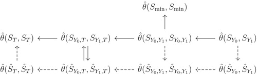
See Figure 1 for difference choices of $S_k$ and Figure A1 for the comparisons of efficiency of estimator $\hat{\theta }$ based on different $S_k$, $k=0,1$.

Appendix 5

Asymptotic variance comparisons between using $S_{Y_0,Y_1}$ and using $S_{Y_k,T}$

In this section, we prove that the asymptotic variance of $\hat{\theta }(S_{Y_0,Y_1},S_{Y_0,Y_1})$ is smaller than asymptotic variance of $\hat{\theta }(S_{Y_0,T},S_{Y_0,T})$, followed by those of $\hat{\theta }(S_T,S_T)$. From the proof of Theorem 2.1, for all $S_k$ satisfying $T\perp Y_k|S_k$, the asymptotic variance of $\hat{\theta }(S_1,S_0)$ is $\begin{array}{rl}& \mathrm{V}\mathrm{a}\mathrm{r}\left\{E\left(g_1\left(Y_1\right)|S_1\right)-E\left(g_0\left(Y_0\right)|S_0\right)\right\}\\ & +E\left\{\frac{\mathrm{V}\mathrm{a}\mathrm{r}\left(g_1\right(Y_1\left)|S_1\right)}{{\pi }_1\left(S_1\right)}\right\}+E\left\{\frac{\mathrm{V}\mathrm{a}\mathrm{r}\left(g_0\right(Y_0\left)|S_0\right)}{{\pi }_0\left(S_0\right)}\right\}.\end{array}$ For $\hat{\theta }(S_{Y_0,Y_1},S_{Y_0,Y_1})$ and $\hat{\theta }(S_{Y_0,T},S_{Y_1,T})$, the asymptotic variances $V_{S_{Y_0,Y_1}}$ and $V_{S_{Y_0,T},S_{Y_1,T}}^{\ast }$ are $\begin{array}{rl}& V_{S_{Y_0,Y_1}}^{\ast }\\ & =\mathrm{V}\mathrm{a}\mathrm{r}\left\{E\left(g_1\left(Y_1\right)|S_{Y_0,Y_1}\right)-E\left(g_0\left(Y_0\right)|S_{Y_0,Y_1}\right)\right\}\\ & +E\left\{\frac{\mathrm{V}\mathrm{a}\mathrm{r}\left(g_1\right(Y_1\left)|S_{Y_0,Y_1}\right)}{{\pi }_1\left(S_{Y_0,Y_1}\right)}\right\}+E\left\{\frac{\mathrm{V}\mathrm{a}\mathrm{r}\left(g_0\right(Y_0\left)|S_{Y_0,Y_1}\right)}{{\pi }_0\left(S_{Y_0,Y_1}\right)}\right\}\\ & =\mathrm{V}\mathrm{a}\mathrm{r}\left\{E\left(g_1\left(Y_1\right)|S_{Y_1}\right)-E\left(g_0\left(Y_0\right)|S_{Y_0}\right)\right\}\\ & +E\left\{\frac{\mathrm{V}\mathrm{a}\mathrm{r}\left(g_1\right(Y_1\left)|S_{Y_1}\right)}{{\pi }_1\left(S_{Y_0,Y_1}\right)}\right\}+E\left\{\frac{\mathrm{V}\mathrm{a}\mathrm{r}\left(g_0\right(Y_0\left)|S_{Y_0}\right)}{{\pi }_0\left(S_{Y_0,Y_1}\right)}\right\}\\ & V_{S_{Y_0,T},S_{Y_1,T}}^{\ast }\\ & =\mathrm{V}\mathrm{a}\mathrm{r}\left\{E\left(g_1\left(Y_1\right)|S_{Y_1,T}\right)-E\left(g_0\left(Y_0\right)|S_{Y_0,T}\right)\right\}\\ & +E\left\{\frac{\mathrm{V}\mathrm{a}\mathrm{r}\left(g_1\right(Y_1\left)|S_{Y_1,T}\right)}{{\pi }_1\left(S_{Y_1,T}\right)}\right\}+E\left\{\frac{\mathrm{V}\mathrm{a}\mathrm{r}\left(g_0\right(Y_0\left)|S_{Y_0,T}\right)}{{\pi }_0\left(S_{Y_0,T}\right)}\right\}\\ & =\mathrm{V}\mathrm{a}\mathrm{r}\left\{E\left(g_1\left(Y_1\right)|S_{Y_1}\right)-E\left(g_0\left(Y_0\right)|S_{Y_0}\right)\right\}\\ & +E\left\{\frac{\mathrm{V}\mathrm{a}\mathrm{r}\left(g_1\right(Y_1\left)|S_{Y_1}\right)}{{\pi }_1\left(S_{Y_1,T}\right)}\right\}+E\left\{\frac{\mathrm{V}\mathrm{a}\mathrm{r}\left(g_0\right(Y_0\left)|S_{Y_0}\right)}{{\pi }_0\left(S_{Y_0,T}\right)}\right\}\\ & =\mathrm{V}\mathrm{a}\mathrm{r}\left\{E\left(g_1\left(Y_1\right)|S_{Y_1}\right)-E\left(g_0\left(Y_0\right)|S_{Y_0}\right)\right\}\\ & +E\left\{\frac{\mathrm{V}\mathrm{a}\mathrm{r}\left(g_1\right(Y_1\left)|S_{Y_1}\right)}{{\pi }_1\left(S_T\right)}\right\}+E\left\{\frac{\mathrm{V}\mathrm{a}\mathrm{r}\left(g_0\right(Y_0\left)|S_{Y_0}\right)}{{\pi }_0\left(S_T\right)}\right\}\end{array}$ Thus we only need to prove $E\left\{\frac{\mathrm{V}\mathrm{a}\mathrm{r}\left(g_1\right(Y_1\left)|S_{Y_1}\right)}{{\pi }_1\left(S_T\right)}\right\}\ge E\left\{\frac{\mathrm{V}\mathrm{a}\mathrm{r}\left(g_1\right(Y_1\left)|S_{Y_1}\right)}{{\pi }_1\left(S_{Y_0,Y_1}\right)}\right\}$ By Jensen's inequity, $\begin{array}{rl}& E\left\{\frac{\mathrm{V}\mathrm{a}\mathrm{r}\left(g_1\right(Y_1\left)|S_{Y_1}\right)}{{\pi }_1\left(S_T\right)}\right\}=E\left\{\frac{\mathrm{V}\mathrm{a}\mathrm{r}\left(g_1\right(Y_1\left)|S_{Y_1}\right)}{{\pi }_1\left(X\right)}\right\}\\ & =E\left\{\left.E\left[\frac{\mathrm{V}\mathrm{a}\mathrm{r}\left(g_1\right(Y_1\left)|S_{Y_1}\right)}{{\pi }_1\left(X\right)}\right|S_{Y_0,Y_1}\right]\right\}\\ & =E\left\{\mathrm{V}\mathrm{a}\mathrm{r}\left(g_1\right(Y_1\left)|S_{Y_1}\right)E\left[\left.\frac{1}{{\pi }_1\left(X\right)}\right|S_{Y_0,Y_1}\right]\right\}\\ & \ge E\left\{\mathrm{V}\mathrm{a}\mathrm{r}\left(g_1\right(Y_1\left)|S_{Y_1}\right)\frac{1}{E\left[{\pi }_1\left(X\right)|S_{Y_0,Y_1}\right]}\right\}\\ & =E\left\{\frac{\mathrm{V}\mathrm{a}\mathrm{r}\left(g_1\right(Y_1\left)|S_{Y_1}\right)}{{\pi }_1\left(S_{Y_0,Y_1}\right)}\right\}\end{array}$ Hence $\hat{\theta }(S_{Y_0,Y_1},S_{Y_0,Y_1})\to \hat{\theta }(S_{Y_0,T},S_{Y_1,T})$. Note that from Lemma A.1 we have $V_{S_{Y_0,T},S_{Y_1,T}}^{\ast }\le V_{X,X}^{\ast }$, i.e. $\hat{\theta }(S_{Y_0,T},S_{Y_1,T})\to \hat{\theta }(X,X)$. Then the other result follows from $\hat{\theta }(X,X)\to \hat{\theta }(S_T,S_T)$, which is proved in the Appendix 4.

Figure A1. Five choices of $S_k$ in the space of all linear combinations of X. For $(S_{Y_0},S_{Y_1})$ and $(S_{Y_0,T},S_{Y_1,T})$, the first row are $S_0$ for estimating $Y_0$ characteristics, the second row are $S_1$ for estimating $Y_1$ characteristics.

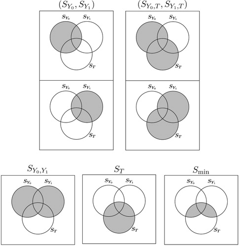
Figure A2. Relative efficiencies of estimators. Solid arrow from A to B means that A is more asymptotically efficient than B. Dashed arrow from A to B means that empirically A is more efficient than B.

References

- Abadie, A., Angrist, J., & Imbens, G. W. (2002). Instrumental variables estimates of the effect of subsidized training on the quantiles of trainee earnings. Econometrica, 70, 91–117. doi: 10.1111/1468-0262.00270
- Bickel, P. J., Klaassen, C. J., Ritov, Y., & Wellner, J. (1993). Efficient and adaptive inference in semiparametric models. Baltimore: Johns Hopkins University Press.
- Brookhart, M., Schneeweiss, S., Rothman, K., Glynn, R., Avorn, J., & Sturmer, T. (2006). Variable selection for propensity score models. American Journal of Epidemiology, 163, 1149–1156. doi: 10.1093/aje/kwj149
- Cattaneo, M. D. (2010). Efficient semiparametric estimation of multi-valued treatment effects under ignorability. Journal of Econometrics, 155, 138–154. doi: 10.1016/j.jeconom.2009.09.023
- Cattaneo, M. D., Drukker, D. M., & Holland, A. D. (2013). Estimation of multivalued treatment effects under conditional independence. The Stata Journal, 13, 407–450. doi: 10.1177/1536867X1301300301
- Chen, X., Wan, A. T. K., & Zhou, Y. (2015). Efficient quantile regression analysis with missing observations. Journal of the American Statistical Association, 110, 723–741. doi: 10.1080/01621459.2014.928219
- Cheng, P. E., & Chu, C. (1996). Kernel estiamation of distribution functions and quantiles with missing data. Statistica Sinica, 6, 63–78.
- Chernozhukov, V., & Hansen, C. (2005). An IV model of quantile treatment effects. Econometrica, 73, 245–261. doi: 10.1111/j.1468-0262.2005.00570.x
- Cook, R. D., & Weisberg, S. (1991). Discussion of ‘Sliced inverse regression for dimension reduction’. Journal of the American Statistical Association, 86, 328–332.
- De Luna, X., Waernbaum, I., & Richardson, T. S. (2011). Covariate selection for the nonparametric estimation of an average treatment effect. Biometrika, 98, 861–875. doi: 10.1093/biomet/asr041
- Doksum, K. (1974). Empirical probability plots and statistical inference for nonlinear models in the two-sample case. The Annals of Statistics, 2, 267–277. doi: 10.1214/aos/1176342662
- Firpo, S. (2007). Efficient semiparametric estimation of quantile treatment effects. Econometrica, 75, 259–276. doi: 10.1111/j.1468-0262.2007.00738.x
- Frölich, M., & Melly, B. (2010). Estimation of quantile treatment effects with Stata. The Stata Journal, 10, 423–457. doi: 10.1177/1536867X1001000309
- Frölich, M., & Melly, B. (2013). Unconditional quantile treatment effects under endogeneity. Journal of Business and Economic Statistics, 31, 346–357. doi: 10.1080/07350015.2013.803869
- Hahn, J. (1998). On the role of the propensity score in efficient semiparametric estimation of average treatment effects. Econometrica, 66, 315–331. doi: 10.2307/2998560
- Hahn, J. (2004). Functional restriction and efficiency in causal inference. Review of Economics and Statistics, 86, 73–76. doi: 10.1162/003465304323023688
- Hardle, W., Muller, M., Sperlich, S., & Werwatz, A. (2004). Nonparametric and semiparametric models. Heidelberg: Springer-Verlag.
- Hsing, T., & Carroll, R. J. (1992). An asymptotic theory for sliced inverse regression. The Annals of Statistics, 20, 1040–1061. doi: 10.1214/aos/1176348669
- Hu, Z., Follmann, D. A., & Wang, N. (2014). Estimation of mean response via the effective balancing score. Biometrika, 101, 613–624. doi: 10.1093/biomet/asu022
- Koenker, R., & Bassett, G. (1978). Regression quantiles. Econometrica, 46, 33–50. doi: 10.2307/1913643
- Lehman, E. L. (1975). Nonparametrics: Statistical methods based on ranks. San Francisco: Holden-Day.
- Li, K. C. (1991). Sliced inverse regression for dimension reduction. Journal of the American Statistical Association, 86, 316–327. doi: 10.1080/01621459.1991.10475035
- Rosenbaum, P. R., & Rubin, D. B. (1983). The central role of the propensity score in observational studies for causal effects. Biometrika, 70, 41–55. doi: 10.1093/biomet/70.1.41
- Shortreed, S. M., & Ertefaie, A. (2017). Outcome-adaptive Lasso: Variable selection for causal inference. Biometrics, 73, 1111–1122. doi: 10.1111/biom.12679
- Silverman, B. W. (1986). Density estimation for statistics and data analysis. London: Chapman and Hall.
- Xia, Y., Tong, H., Li, W. K., & Zhu, L. X. (2002). An adaptive estimation of dimension reduction space. Journal of the Royal Statistical Society: Series B (Statistical Methodology), 64, 363–410. doi: 10.1111/1467-9868.03411
- Zhou, Y., Wan, A. T. K., & Wang, X. (2008). Estimating equations inference with missing data. Journal of the American Statistical Association, 103, 1187–1199. doi: 10.1198/016214508000000535
- Zhu, L. X., & Ng, K. W. (1995). Asymptotics of sliced inverse regression. Statistica Sinica, 5, 727–736.
- Zhu, L. P., Zhu, L. X., & Feng, Z. H. (2010). Dimension reduction in regressions through cumulative slicing estimation. Journal of the American Statistical Association, 105, 1455–1466. doi: 10.1198/jasa.2010.tm09666