Efficient estimation of smoothing spline with exact shape constraints

ABSTRACT

Smoothing spline is a popular method in non-parametric function estimation. For the analysis of data from real applications, specific shapes on the estimated function are often required to ensure the estimated function undeviating from the domain knowledge. In this work, we focus on constructing the exact shape constrained smoothing spline with efficient estimation. The ‘exact’ here is referred as to impose the shape constraint on an infinite set such as an interval in one-dimensional case. Thus the estimation becomes a so-called semi-infinite optimisation problem with an infinite number of constraints. The proposed method is able to establish a sufficient and necessary condition for transforming the exact shape constraints to a finite number of constraints, leading to efficient estimation of the shape constrained functions. The performance of the proposed methods is evaluated by both simulation and real case studies.

Keywords:

• Monotonicity
• non-linear constraint
• non-parametric regression

1. Introduction

In recent years, non-parametric smoothing methods have gained popularity in various science and engineering areas such as economics, biology, smart manufacturing, etc. One advantage of these methods is that they do not assume strong parametric structure for the underlying model. While in the analysis of data from real applications, researchers often demand a specific shape on the estimated function to ensure the estimated function undeviating from their domain knowledge. For example, shape with monotonicity are often required in the estimation of dose-response function (Kelly & Rice, 1990) in medicine. The degradation curve of scaffolds in engineered scaffold fabrication often requires to be monotonic and concave (Zeng, Deng, & Yang, 2016). The estimation of human growth curve (Ducharme & Fontez, 2004) in biometrics and estimation of utility function (Matzkin, 1991) in economics often needs the concavity in shape.

Among various non-parametric smoothers, spline smoothing and kernel smoothing are quite popular. Theoretical and numerical properties of these techniques have been well studied. See Wahba (1990) and Green and Silverman (1993) for thorough discussions of the spline smoothing problem, and Fan and Gijbels (1996) and Wand and Jones (1995) for the kernel smoothing problem. Unlike its unconstrained counterpart, shape constrained smoother has not received large attentions in the statistics literature. As pointed in Delecroix and Thomas-Agnan (2000), most of the isotonic estimates are based on splines rather than on kernels since enforcing the restrictions at the minimisation step appears to be a natural solution.

There are various splines to enable the shape constraints. For example, B-spline is a popular approach because of its special properties: non-decreasing coefficients imply non-decreasing resulting function (Brezger & Steiner, 2003; Dierckx, 1980; He & Shi, 1998; Kelly & Rice, 1990). There are also I-spline methods (Curry & Schoenberg, 1966; Ramsay, 1988) to integrate over non-negative M-splines for constructing monotone smoothers. Meyer (2008) defined the C-splines that at each observation to impose the shape constraint. Combinations of monotonicity and convexity can be imposed by the regression splines. Meyer (2012) also developed penalised splines under shape constraints. (Liao & Meyer, 2017) proposed estimators of change-point based on constrained splines. Meyer (2018) proposed the constrained generalised additive model using iteratively reweighted cone projection algorithm. The smoothing spline is another popular approach, of which the most notable works include (Wang & Li, 2008)'s second order cone programming to create monotone smoothing spline and (Turlach, 2005)'s approach of adaptively adding constraints to create shape constrained smoothing spline.

In this work, we consider the smoothing spline to study the exact shape constraints. Here the meaning of ‘exact’ is referred as to impose the shape constraint on an infinite set such as an interval in one-dimensional case. It leads to a so-called semi-infinite optimisation problem with an infinite number of constraints. Suppose that the observational data are $(x_i,y_i)$ for $i=1,\dots ,n$, and we assume $L\le x_1<\cdots <x_n\le U$. The exact shape constrained smoothing spline is defined as the solution of the following optimisation problem: (1a) $\begin{array}{rl}& \underset{f}{\mathrm{m}\mathrm{i}\mathrm{n}\mathrm{i}\mathrm{m}\mathrm{i}\mathrm{s}\mathrm{e}}\sum _{i=1}^n(y_i-f(x_i){)}^2+\lambda {\int }_a^b[f^{\left(2\right)}\left(t\right){]}^2\mathrm{d}t,\end{array}$(1a) (1b) $\begin{array}{rl}& \mathrm{s}\mathrm{u}\mathrm{b}\mathrm{j}\mathrm{e}\mathrm{c}\mathrm{t}\mathrm{t}\mathrm{o}{f}^{\left(r\right)}\left(x\right)\ge 0\mathrm{f}\mathrm{o}\mathrm{r}x\in [L,U],\end{array}$(1b) where $f^{\left(r\right)}\left(x\right)$ is the rth derivative of $f\left(x\right)$ and $\lambda \ge 0$ is a tuning parameter. The formulation in (1a(1a) $\begin{array}{rl}& \underset{f}{\mathrm{m}\mathrm{i}\mathrm{n}\mathrm{i}\mathrm{m}\mathrm{i}\mathrm{s}\mathrm{e}}\sum _{i=1}^n(y_i-f(x_i){)}^2+\lambda {\int }_a^b[f^{\left(2\right)}\left(t\right){]}^2\mathrm{d}t,\end{array}$(1a) ) without constraint is the well-known smoothing spline problem, the solution of which is known as the cubic smoothing spline over the class of twice differential functions. The framework for r = 1 and r = 2 corresponds to the monotone non-decreasing and convex shape constraint, respectively. The monotone decreasing or concave constraint can be easily obtained by reversing the inequality sign in (1b(1b) $\begin{array}{rl}& \mathrm{s}\mathrm{u}\mathrm{b}\mathrm{j}\mathrm{e}\mathrm{c}\mathrm{t}\mathrm{t}\mathrm{o}{f}^{\left(r\right)}\left(x\right)\ge 0\mathrm{f}\mathrm{o}\mathrm{r}x\in [L,U],\end{array}$(1b) ). One can pursue either one of the constraints or some of them under this framework. For example, non-global constraint, such as convex for $x\le 0$ and concave for x>0 is possible. A mixed constraint, such as combination of concave and monotone increasing, can also be applied.

The challenges for the estimation in (1(1a) $\begin{array}{rl}& \underset{f}{\mathrm{m}\mathrm{i}\mathrm{n}\mathrm{i}\mathrm{m}\mathrm{i}\mathrm{s}\mathrm{e}}\sum _{i=1}^n(y_i-f(x_i){)}^2+\lambda {\int }_a^b[f^{\left(2\right)}\left(t\right){]}^2\mathrm{d}t,\end{array}$(1a) ) is the constraints are defined on an infinite set, which implies an infinite number of constraints. By taking advantage of the close connection between the natural cubic spline and the smoothing spline, the proposed method utilises a good representation of smoothing spline to establish a sufficient and necessary condition for transforming the exact shape constraints in (1b(1b) $\begin{array}{rl}& \mathrm{s}\mathrm{u}\mathrm{b}\mathrm{j}\mathrm{e}\mathrm{c}\mathrm{t}\mathrm{t}\mathrm{o}{f}^{\left(r\right)}\left(x\right)\ge 0\mathrm{f}\mathrm{o}\mathrm{r}x\in [L,U],\end{array}$(1b) ) to a finite number of constraints. The resultant solution to the case of r = 2 is straightforward, and the challenge arises when r = 1. To the best of our knowledge, an exact solution for r = 1 has yet to be found in the literature. To facilitate the computation of parameter estimation, we also develop efficient algorithm based on matrix approximation for the large data.

The remaining paper is organised as follows. Section 2 revisits the connection between the natural cubic splines and smoothing splines. The proposed exact shape-constraint smoothing spline is detailed in Section 3. An efficient computation algorithm for parameter estimation are developed in Section 4. Sections 5 and 6 evaluate the performance of the proposed method from a simulation study and an application to real life data. We conclude this work with some discussion in Section 7.

2. Revisit of natural cubic spline and smoothing spline

The natural cubic spline (NCS) plays an essential role for the smoothing spline. Suppose that the observed data are $(x_1,y_1),\dots ,(x_n,y_n)$ with $x_1<\cdots <x_n$. An NCS function $f\left(x\right)$ with knots at $x_1,\dots ,x_n$ is a piecewise polynomial of degree up to three with breakpoints at $x_1,\dots ,x_n$. In addition, $f\left(x\right)$ is twice continuously differentiable at the knots and linear beyond the boundary.

Let $f\left(x\right)$ be a NCS with knots at $x_1,\dots ,x_n$. By definition, $f\left(x\right)$ can be expressed as (2a) $\begin{array}{rl}& f\left(x\right)=\left\{\begin{array}{ll}{f}_0\left(x\right)=c_{0}x+d_0,& x<x_1,\\ f_i\left(x\right)=a_i{x}^3\\ +b_i{x}^2+c_{i}x+d_i,& x_i\le x<x_{i+1}\\ & \mathrm{f}\mathrm{o}\mathrm{r}i=1,\dots ,n-1,\\ f_n\left(x\right)=c_{n}x+d_n,& x\ge x_n,\end{array}\right.\end{array}$(2a) (2b) $\begin{array}{rl}& \mathrm{w}\mathrm{i}\mathrm{t}\mathrm{h}\mathrm{r}\mathrm{e}\mathrm{s}\mathrm{t}\mathrm{r}\mathrm{i}\mathrm{c}\mathrm{t}\mathrm{i}\mathrm{o}\mathrm{n}\mathrm{s}\\ f_i\left(x_{i+1}\right)& =f_{i+1}\left(x_{i+1}\right),f_i^{\prime }\left(x_{i+1}\right)=f_{i+1}^{\prime }\left(x_{i+1}\right),f_i^{″}\left(x_{i+1}\right)\\ & =f_{i+1}^{″}\left(x_{i+1}\right)\mathrm{f}\mathrm{o}\mathrm{r}i=0,\dots ,n-1.\end{array}$(2b) The derivatives of $f\left(x\right)$ can be obtained by taking derivative on each polynomial and maintaining the relevant constraints. Please refer to Appendix 1 for explicit expressions. This piecewise polynomial representation of an NCS in (2(2a) $\begin{array}{rl}& f\left(x\right)=\left\{\begin{array}{ll}{f}_0\left(x\right)=c_{0}x+d_0,& x<x_1,\\ f_i\left(x\right)=a_i{x}^3\\ +b_i{x}^2+c_{i}x+d_i,& x_i\le x<x_{i+1}\\ & \mathrm{f}\mathrm{o}\mathrm{r}i=1,\dots ,n-1,\\ f_n\left(x\right)=c_{n}x+d_n,& x\ge x_n,\end{array}\right.\end{array}$(2a) ) is a key for formulating the shape constraints in Section 3. For estimation of $f\left(x\right)$, however, there exists another presentation for computational purpose. Specifically, we first estimate $f\left(x_1\right),\dots ,f\left(x_n\right)$ by writing them as a linear combination of specific basis functions and estimate the corresponding coefficients. Then we can utilise the value-second derivative representation (Green & Silverman, 1993) to recover the entire function $f\left(x\right)$. As a result, the problem in (1a(1a) $\begin{array}{rl}& \underset{f}{\mathrm{m}\mathrm{i}\mathrm{n}\mathrm{i}\mathrm{m}\mathrm{i}\mathrm{s}\mathrm{e}}\sum _{i=1}^n(y_i-f(x_i){)}^2+\lambda {\int }_a^b[f^{\left(2\right)}\left(t\right){]}^2\mathrm{d}t,\end{array}$(1a) ) can be converted into a ridge regression-like problem that can be efficiently solved.

Let ${\mathbf{1}}_n$ be length-n vector of ones, $\mathit{x}=(x_1,\dots ,x_n{)}^T$ and $\mathit{g}=\left(f\right(x_1),\dots ,f(x_n){)}^T$. Without loss of generality, we assume $\mathit{x}$ is centred with zero mean. We can construct the banded matrices $\mathit{Q}$ and $\mathit{R}$ according to Equations (A1(A1) $\begin{array}{rl}\mathit{Q}& =\left(\begin{array}{ccc}{h}_1^{-1}& & \\ -h_1^{-1}-h_2^{-1}& \ddots & 0\\ h_2^{-1}& \ddots & \\ & \ddots & h_{n-2}^{-1}\\ 0& & -h_{n-2}^1-h_{n-1}^{-1}\\ & & h_{n-1}^{-1}\end{array}\right),\end{array}$(A1) ) and (A2(A2) $\begin{array}{rl}\mathit{R}& =\left(\begin{array}{cccc}\frac{1}{3}(h_1+h_2)& \frac{1}{6}{h}_2& & 0\\ \frac{1}{6}{h}_2& \ddots & \ddots & \\ & \ddots & \ddots & \frac{1}{6}{h}_{n-2}\\ 0& & \frac{1}{6}{h}_{n-2}& \frac{1}{3}(h_{n-2}+h_{n-1})\end{array}\right),\end{array}$(A2) ) in Appendix A.2. The linear mixed model representation described in Appendix A.3 allows us to rewrite the NCS formulation in (2(2a) $\begin{array}{rl}& f\left(x\right)=\left\{\begin{array}{ll}{f}_0\left(x\right)=c_{0}x+d_0,& x<x_1,\\ f_i\left(x\right)=a_i{x}^3\\ +b_i{x}^2+c_{i}x+d_i,& x_i\le x<x_{i+1}\\ & \mathrm{f}\mathrm{o}\mathrm{r}i=1,\dots ,n-1,\\ f_n\left(x\right)=c_{n}x+d_n,& x\ge x_n,\end{array}\right.\end{array}$(2a) ) as (3) $\mathit{g}={\mathbf{1}}_n{\theta }_0+\mathit{x}{\theta }_1+\mathit{A}\text{β},$(3) here $\mathit{A}=\mathit{Q}({\mathit{Q}}^T\mathit{Q}{)}^{-1}{\mathit{R}}^{1/2}\in {\mathbb{R}}^{n\times (n-2)}$. The ${\theta }_1,{\theta }_2$ and $\text{β}=({\text{β}}_1,\dots ,{\text{β}}_{n-2}{)}^{\prime }$ are parameters. By construction, matrix $\mathit{A}$ has full rank. It is easy to check that ${\mathbf{1}}_n^T\mathit{x}=0$, ${\mathbf{1}}_n^T\mathit{A}=0$ and ${\mathit{x}}^T\mathit{A}=0$. Hence $\{{\mathbf{1}}_n,\mathit{x},\mathit{A}\}$ form a basis of the n-dimensional euclidean space. Furthermore, if we define matrix $\mathit{K}=\mathit{Q}{\mathit{R}}^{-1}{\mathit{Q}}^T\in {\mathbb{R}}^{n\times n}$, then we get: (4) $\int \left[f^{″}\right(t){]}^2\mathrm{d}t={\mathit{g}}^T\mathit{K}\mathit{g}={\text{β}}^T\text{β}.$(4) It is worth to pointing out that the underlying model for the smoothing spline can be considered as a natural cubic spline with knots at $x_1,\dots ,x_n$ and at most $k=2\left[n/2\right]+2$ additional knots of which the locations are unknown (Utreras, 1985). Here we made a mild assumption that $f\left(x\right)$ is a natural cubic spline with knots at $x_1,\dots ,x_n$. Combining this assumption with results in (3(3) $\mathit{g}={\mathbf{1}}_n{\theta }_0+\mathit{x}{\theta }_1+\mathit{A}\text{β},$(3) ) and (4(4) $\int \left[f^{″}\right(t){]}^2\mathrm{d}t={\mathit{g}}^T\mathit{K}\mathit{g}={\text{β}}^T\text{β}.$(4) ), the smoothing spline expressed in (1a(1a) $\begin{array}{rl}& \underset{f}{\mathrm{m}\mathrm{i}\mathrm{n}\mathrm{i}\mathrm{m}\mathrm{i}\mathrm{s}\mathrm{e}}\sum _{i=1}^n(y_i-f(x_i){)}^2+\lambda {\int }_a^b[f^{\left(2\right)}\left(t\right){]}^2\mathrm{d}t,\end{array}$(1a) ) is equivalent to the problem of (5a) $\underset{({\theta }_0,{\theta }_1,\text{β})}{\mathrm{m}\mathrm{i}\mathrm{n}\mathrm{i}\mathrm{m}\mathrm{i}\mathrm{s}\mathrm{e}}\sum _{i=1}^n(y_i-{\theta }_0-x_i{\theta }_1-{\mathit{A}}_i\text{β}{)}^2+{\lambda }_1{\text{β}}^T\text{β},$(5a) where ${\mathit{A}}_i$ is the ith row of matrix $\mathit{A}$. This is simply a ridge regression problem with response vector $\mathit{y}$ and covariates matrix $({\mathbf{1}}_n,\mathit{x},\mathit{A})$ without penalising ${\theta }_0$ and ${\theta }_1$.

When one obtain the estimate of $\mathit{\theta }=({\theta }_0,{\theta }_1,\mathit{b}{)}^T$, the entire estimated function can be constructed by following the procedure in Appendix A.3. one can actually obtain the piecewise polynomial representation of the estimated function by following the steps in Appendix A.4. That is, the piecewise polynomial representation is fully specified when $({\theta }_1,{\theta }_2,\text{β})$ are known.

3. Exact shape-constrained smoothing spline

To have the exact shape constraint, one major difficulty is that the inequality constraint in (1b(1b) $\begin{array}{rl}& \mathrm{s}\mathrm{u}\mathrm{b}\mathrm{j}\mathrm{e}\mathrm{c}\mathrm{t}\mathrm{t}\mathrm{o}{f}^{\left(r\right)}\left(x\right)\ge 0\mathrm{f}\mathrm{o}\mathrm{r}x\in [L,U],\end{array}$(1b) ) cannot be guaranteed by simply enforcing constraints at $x_1,\dots ,x_n$. Due to these challenges, many computable ‘solutions’ to the shape constrained smoothing spline problem described in ((1a(1a) $\begin{array}{rl}& \underset{f}{\mathrm{m}\mathrm{i}\mathrm{n}\mathrm{i}\mathrm{m}\mathrm{i}\mathrm{s}\mathrm{e}}\sum _{i=1}^n(y_i-f(x_i){)}^2+\lambda {\int }_a^b[f^{\left(2\right)}\left(t\right){]}^2\mathrm{d}t,\end{array}$(1a) ) and (1b(1b) $\begin{array}{rl}& \mathrm{s}\mathrm{u}\mathrm{b}\mathrm{j}\mathrm{e}\mathrm{c}\mathrm{t}\mathrm{t}\mathrm{o}{f}^{\left(r\right)}\left(x\right)\ge 0\mathrm{f}\mathrm{o}\mathrm{r}x\in [L,U],\end{array}$(1b) )) are approximations of some kind. Some approximate by assuming the resulting function being a natural cubic spline with knots at all data points (Turlach, 2005; Wang & Li, 2008), others approximate by discretisation of infinite constraint (1b(1b) $\begin{array}{rl}& \mathrm{s}\mathrm{u}\mathrm{b}\mathrm{j}\mathrm{e}\mathrm{c}\mathrm{t}\mathrm{t}\mathrm{o}{f}^{\left(r\right)}\left(x\right)\ge 0\mathrm{f}\mathrm{o}\mathrm{r}x\in [L,U],\end{array}$(1b) ) to a finite number of constraints (Mammen & Thomas-Agnan, 1999; Nagahara & Martin, 2013; Villalobos & Wahba, 1987).

It is known that the solution to the exact shape-constraint smoothing spline in (1a) and (1b) is a natural cubic spline with knots at $x_1,\dots ,x_n$ and at most $k=2\left[n/2\right]+2$ additional knots of which the locations are unknown as proved in Theorem 3.3 in (Utreras, 1985). Unfortunately, it does not provide much practical use because of the unknown locations of those additional knots. However, it sheds some lights that a natural cubic spline with knots at all data points is an adequate approximation to the theoretically correct model proved by Utreras (1985). Therefore, we develop our proposed method under the consideration that the estimated model is a natural cubic spline with knots at all data points. Specifically, we propose a representation only using n−1 constraints that is equivalent to the infinite constraint (1b(1b) $\begin{array}{rl}& \mathrm{s}\mathrm{u}\mathrm{b}\mathrm{j}\mathrm{e}\mathrm{c}\mathrm{t}\mathrm{t}\mathrm{o}{f}^{\left(r\right)}\left(x\right)\ge 0\mathrm{f}\mathrm{o}\mathrm{r}x\in [L,U],\end{array}$(1b) ) for $r=1\mathrm{o}\mathrm{r}2$. Compared to Turlach (2005) who took an adaptive approach to adding constraints and thus changing the underlying quadratic program for parameter estimation, the proposed method optimises over a larger underlying model space yet it maintains the exactness of the shape constraint. Different from Wang Li (2008) who only works on monotonicity constraint (r = 1), our proposed method also works on convexity constraint (r = 2) and can easily be extended to mixed and non-global constraint.

The key idea of our proposed method is to utilise the piecewise polynomial representation of NCS to provide a sufficient and necessary condition in converting constraint (1b(1b) $\begin{array}{rl}& \mathrm{s}\mathrm{u}\mathrm{b}\mathrm{j}\mathrm{e}\mathrm{c}\mathrm{t}\mathrm{t}\mathrm{o}{f}^{\left(r\right)}\left(x\right)\ge 0\mathrm{f}\mathrm{o}\mathrm{r}x\in [L,U],\end{array}$(1b) ) for r = 2 and r = 1 to the form of $c(\mathit{\theta };\mathit{x})⪰\mathbf{0}$, where we define notation ≽ as element-wise greater than or equal to. Then we can express the shape constrained smoothing spline problem as (5a) $\begin{array}{rl}& \underset{({\theta }_0,{\theta }_1,\text{β})}{\mathrm{m}\mathrm{i}\mathrm{n}\mathrm{i}\mathrm{m}\mathrm{i}\mathrm{s}\mathrm{e}}\sum _{i=1}^n(y_i-{\theta }_0-x_i{\theta }_1-{\mathit{A}}_i\text{β}{)}^2+{\lambda }_1{\text{β}}^T\text{β},\end{array}$(5a) (5b) $\begin{array}{rl}& \mathrm{s}\mathrm{u}\mathrm{b}\mathrm{j}\mathrm{e}\mathrm{c}\mathrm{t}\mathrm{t}\mathrm{o}c(\mathit{\theta };\mathit{x})⪰\mathbf{0}.\end{array}$(5b) The formulation above can be optimised by many standard optimisation methods that take non-linear constraints.

The shape constraint (1b(1b) $\begin{array}{rl}& \mathrm{s}\mathrm{u}\mathrm{b}\mathrm{j}\mathrm{e}\mathrm{c}\mathrm{t}\mathrm{t}\mathrm{o}{f}^{\left(r\right)}\left(x\right)\ge 0\mathrm{f}\mathrm{o}\mathrm{r}x\in [L,U],\end{array}$(1b) ) for r = 1 (monotonicity) and r = 2 (convexity) are presented below as Theorems 3.1 and 3.2, respectively. The mixed constraints can be achieved by combining the corresponding constraints.

Theorem 3.1

For the smoothing spline, the monotone non-decreasing constraint, defined as $f^{\prime }\left(x\right)\ge 0,$ holds if and only if constraint (5b(5b) $\begin{array}{rl}& \mathrm{s}\mathrm{u}\mathrm{b}\mathrm{j}\mathrm{e}\mathrm{c}\mathrm{t}\mathrm{t}\mathrm{o}c(\mathit{\theta };\mathit{x})⪰\mathbf{0}.\end{array}$(5b) ) with (6) $\begin{array}{rl}& c(\mathit{\theta };\mathit{x})=\left(c_1\right(\mathit{\theta };\mathit{x}),\dots ,c_{n-1}(\mathit{\theta };\mathit{x}){)}^T,\\ & where\\ & c_i(\mathit{\theta };\mathit{x})=\left\{\begin{array}{l}min\left(f^{\prime }\left(x_i\right),f^{\prime }\left(x_{i+1}\right),f^{\prime }\left(\frac{-b_i}{3a_i}\right)\right),\\ if\frac{-b_i}{3a_i}\in (x_i,x_{i+1})and{a}_i>0\\ min\left(f^{\prime }\right(x_i),f^{\prime }(x_{i+1}\left)\right),otherwise\end{array}\right.\end{array}$(6) holds.

Proof.

Based on the polynomial representation of NCS, it is easy to get the first derivative $f^{\prime }\left(x\right)$ as (7) $\begin{array}{rl}& f^{\prime }\left(x\right)=\left\{\begin{array}{ll}{f}_0^{\prime }\left(x\right)=c_0,& x<x_1,\\ f_i^{\prime }\left(x\right)=3a_i{x}^2\\ +2b_{i}x+c_i,& x_i\le x<x_{i+1}\mathrm{f}\mathrm{o}\mathrm{r}\\ & i=1,\dots ,n-1,\\ f_n^{\prime }\left(x\right)=c_n,& x\ge x_n,\end{array}\right.\\ & \mathrm{w}\mathrm{i}\mathrm{t}\mathrm{h}\mathrm{r}\mathrm{e}\mathrm{s}\mathrm{t}\mathrm{r}\mathrm{i}\mathrm{c}\mathrm{t}\mathrm{i}\mathrm{o}\mathrm{n}\mathrm{s}{f}_i^{\prime }\left(x_{i+1}\right)=f_{i+1}^{\prime }\left(x_{i+1}\right),f_i^{″}\left(x_{i+1}\right)\\ & =f_{i+1}^{″}\left(x_{i+1}\right),\mathrm{f}\mathrm{o}\mathrm{r}i=0,\dots ,n-1.\end{array}$(7) Clearly, $f^{\prime }\left(x\right)$ is a continuous piecewise polynomial of at most second order on each interval $[x_1,x_2)$,…, $[x_{n-1},x_n)$, and constant on the boundary interval $(-\mathrm{\infty },x_1)$, and $[x_n,\mathrm{\infty })$. For $i=1,\dots ,n-1$, if $a_i=0$, $f_i^{\prime }\left(x\right)$ is a linear function on $[x_i,x_{i+1})$, so $f^{\prime }\left(x\right)\ge min\left(f^{\prime }\right(x_i),f^{\prime }(x_{i+1}\left)\right)$ on the interval. If $a_i\ne 0$, $f_i^{\prime }\left(x\right)$ is a parabola on $[x_i,x_{i+1})$ with stationary point at $-b_i/3a_i$, specifically

1. if $a_i<0$, $f_i^{\prime }\left(x\right)$ is concave. So regardless of the location of the stationary point, $f^{\prime }\left(x\right)\ge min\left(f^{\prime }\right(x_i),f^{\prime }(x_{i+1}\left)\right)$ on $[x_i,x_{i+1})$.

2. if $a_i>0$, $f_i^{\prime }\left(x\right)$ is a convex parabola where the stationary point may or may not lie on $[x_i,x_{i+1})$.

   1. If the stationary point is not on the interval, $f_i^{\prime }\left(x\right)$ is monotone on $[x_i,x_{i+1})$, so $f^{\prime }\left(x\right)\ge min\left(f^{\prime }\right(x_i),f^{\prime }(x_{i+1}\left)\right)$ on the interval.

   2. If the stationary point is on the interval, global minimum could be at either the boundary or the stationary point, so $f^{\prime }\left(x\right)\ge min\left(f^{\prime }\right(x_i),f^{\prime }(x_{i+1}),f^{\prime }(-b_i/3a_i\left)\right)$ on the interval.

Non-negativity on the boundary interval $(-\mathrm{\infty },x_1)$ and $[x_n,\mathrm{\infty })$ hold if $c_0\ge 0$ and $c_n\ge 0$. But no extra constraint is needed because by continuity of $f^{\prime }\left(x\right)$, $c_0=f_1^{\prime }\left(x_1\right)$ and $c_n=f_{n-1}^{\prime }\left(x_n\right)$, non-negativitiy is already ensured by $c_1(\mathit{\theta };\mathit{x})\ge 0$ and $c_{n-1}(\mathit{\theta };\mathit{x})\ge 0$.

If $c(\mathit{\theta },\mathit{x})⪰\mathbf{0}$, then each piecewise polynomial, $f_i^{\prime }\left(x\right)$ for $i=0,\dots ,n$, is non-negative, which in turn implies that the whole function $f^{\prime }\left(x\right)$ must be non-negative. Therefore, validity of inequality (6b(5b) $\begin{array}{rl}& \mathrm{s}\mathrm{u}\mathrm{b}\mathrm{j}\mathrm{e}\mathrm{c}\mathrm{t}\mathrm{t}\mathrm{o}c(\mathit{\theta };\mathit{x})⪰\mathbf{0}.\end{array}$(5b) ) implies the monotone non-decreasing constraint.

The other direction is obvious by definition.

Theorem 3.2

For the smoothing spline, the convexity constraint, defined as $f^{\prime }\left(x\right)\ge 0$, holds if and only if constraint (5b(5b) $\begin{array}{rl}& \mathrm{s}\mathrm{u}\mathrm{b}\mathrm{j}\mathrm{e}\mathrm{c}\mathrm{t}\mathrm{t}\mathrm{o}c(\mathit{\theta };\mathit{x})⪰\mathbf{0}.\end{array}$(5b) ) with (8) $\begin{array}{rl}& c(\mathit{\theta };\mathit{x})=\left(c_1\right(\mathit{\theta };\mathit{x}),\dots ,c_{n-1}(\mathit{\theta };\mathit{x}){)}^T,\\ & \mathrm{w}\mathrm{h}\mathrm{e}\mathrm{r}\mathrm{e}\\ & c_i(\mathit{\theta };\mathit{x})=min\left(f^{″}\right(x_i),f^{″}(x_{i+1}\left)\right),\end{array}$(8) holds.

Proof.

Based on the polynomial representation of NCS, it is easy to get the first derivative $f^{″}\left(x\right)$ as (9) $\begin{array}{rl}& f^{″}\left(x\right)\\ & =\left\{\begin{array}{ll}{f}_0^{″}\left(x\right)=0,& x<x_1,\\ f_i^{″}\left(x\right)=6a_{i}x+2b_i,& x_i\le x<x_{i+1}\mathrm{f}\mathrm{o}\mathrm{r}\\ & i=1,\dots ,n-1,\\ f_n^{″}\left(x\right)=0,& x\ge x_n,\end{array}\right.\\ & \mathrm{w}\mathrm{i}\mathrm{t}\mathrm{h}\mathrm{r}\mathrm{e}\mathrm{s}\mathrm{t}\mathrm{r}\mathrm{i}\mathrm{c}\mathrm{t}\mathrm{i}\mathrm{o}\mathrm{n}\mathrm{s}{f}_i^{″}\left(x_{i+1}\right)=f_{i+1}^{″}\left(x_{i+1}\right),\\ \mathrm{f}\mathrm{o}\mathrm{r}i& =0,\dots ,n-1.\end{array}$(9) The $f^{″}\left(x\right)$ is a continuous piecewise linear polynomial on each interval $(-\mathrm{\infty },x_1)$, $[x_1,x_2)$,…, $[x_{n-1},x_n)$ and $[x_n,\mathrm{\infty })$. Since $f^{″}\left(x\right)=0$ for any $x\le x_1$ and $x\ge x_n$, we only need to consider $f^{″}\left(x\right)$ when $x\in (x_1,x_n)$. For any i, linearity of $f_i^{″}\left(x\right)$ implies $f^{″}\left(x\right)\ge min\left(f^{″}\right(x_i),f^{″}(x_{i+1}\left)\right)$ on interval $[x_i,x_{i+1})$. If $c(\mathit{\theta };\mathit{x})⪰\mathbf{0}$, each piecewise polynomial, $f_i^{″}\left(x\right)$ for $i=0,\dots ,n$, is non-negative, which in turn implies that the whole function $f^{″}\left(x\right)$ is non-negative. Therefore, inequality (6b(5b) $\begin{array}{rl}& \mathrm{s}\mathrm{u}\mathrm{b}\mathrm{j}\mathrm{e}\mathrm{c}\mathrm{t}\mathrm{t}\mathrm{o}c(\mathit{\theta };\mathit{x})⪰\mathbf{0}.\end{array}$(5b) ) implies convexity constraint.

The other direction is obvious by definition.

The above theorems are defined for global constraint, i.e. constraint that holds on the entire domain of the function $[L,U]$. To extend the results to mixed constraint and non-global constraint, we can easily apply Theorem 3.2 and Theorem 3.1 to different local intervals $[L_j,U_j]$, where $L\le L_j\le U_j\le U$. In addition, we can impose up to second-order smooth constraint on the boundary of local intervals. A general procedure is described as follows:

1. Let $L_i$ for $i=1,\dots ,M$ be the points where monotonicity/convexity changes, and $L_0=L$ and $L_{M+1}=U$. Partition the domain of $f\left(x\right)$ into $(L_0,L_1],\dots ,(L_M,L_{M+1})$. As a result, $f\left(x\right)$ on each interval only requires one shape constraint.

2. For each interval, impose constraint according to Theorem 3.2 and Theorem 3.1.

3. For $i=1,\dots ,M$, add $f^{\prime }\left(L_i\right)=0$ for monotone constraint or $f^{″}\left(L_i\right)=0$ for convexity constraint.

The importance of Step 3 is that it can prevent the stationary/inflection point of the estimated function from floating between the knots immediately smaller and larger than the point where monotonicity/convexity changes.

4. Efficient algorithm for parameter estimation

Note that the optimisation problem described in (6a(5a) $\begin{array}{rl}& \underset{({\theta }_0,{\theta }_1,\text{β})}{\mathrm{m}\mathrm{i}\mathrm{n}\mathrm{i}\mathrm{m}\mathrm{i}\mathrm{s}\mathrm{e}}\sum _{i=1}^n(y_i-{\theta }_0-x_i{\theta }_1-{\mathit{A}}_i\text{β}{)}^2+{\lambda }_1{\text{β}}^T\text{β},\end{array}$(5a) ) and (6b(5b) $\begin{array}{rl}& \mathrm{s}\mathrm{u}\mathrm{b}\mathrm{j}\mathrm{e}\mathrm{c}\mathrm{t}\mathrm{t}\mathrm{o}c(\mathit{\theta };\mathit{x})⪰\mathbf{0}.\end{array}$(5b) ) is a quadratic programming with non-linear constraints. Using Python, our implementation algorithm is based on the ralg solver under the OpenOPT platform. The ralg solver resembles the quasi-Newton Method with adaptive space dilation developed by Shor and Zhurbenko (1971). Two advantages for this choice are that it accepts user-provided first-derivative and allows large number of constraints.

4.1. Computation of large data

When the number of observation n is large, the growing dimension of the $n\times (n-2)$ matrix $\mathit{A}$ and vector of constraints $c(\mathit{\theta };\mathit{x})$ are the bottleneck for efficient computation. To address this challenge, we consider to approximate the matrix $\mathit{A}$ by a $n\times K$ dimensional matrix ${\mathit{A}}^{\ast }$, where $K\le n-2$ is independent of n. It also allows the dimension of $\mathit{\theta }$ to be some fixed integer $K+2\le n$.

Following Wand and Ormerod's (2008) mixed model formulation in the semiparametric regression, we adopt a good way to approximate $\mathit{A}$ with ${\mathit{A}}^{\mathbf{\ast }}=\mathit{B}\mathit{L}$, where $\mathit{B}$ is an $n\times (K+4)$ matrix and $\mathit{L}$ is an $(K+4)\times (K+2)$ matrix.

The construction of $\mathit{B}$ is described as follows. First we define ${\kappa }_1,\dots ,{\kappa }_{K+8}$ as $\begin{array}{rl}a& ={\kappa }_1={\kappa }_2={\kappa }_3={\kappa }_4=x_1-ϵ,{\kappa }_5=x_1,\\ & {\kappa }_6,\dots ,{\kappa }_{K+3}\text{ to be the }\\ & \times \left(\frac{1}{K+1},\frac{2}{K+1},\dots ,\frac{K}{K+1}\right)\\ & \times {100}^{th}\text{ percentile of }{x}_1,\dots ,x_n,\\ {\kappa }_{K+4}& =x_n,b={\kappa }_{K+5}={\kappa }_{K+6}\\ & ={\kappa }_{K+7}={\kappa }_{K+8}=x_n+ϵ.\end{array}$ Then we construct B-spline basis functions (Hastie, Tibshirani, & Friedman, 2001) $B_{1,4}\left(x\right),\dots ,B_{K+4,4}\left(x\right)$ based on knots sequence ${\kappa }_1,\dots ,{\kappa }_{K+8}$ as $\begin{array}{r}{B}_{i,1}\left(x\right)=\left\{\begin{array}{ll}1& \text{if }x\in [{\kappa }_i,{\kappa }_{i+1})\\ 0& \text{otherwise},\end{array}\right.\end{array}$ for $i=1,\dots ,K+7$, and $\begin{array}{rl}{B}_{i,m}\left(x\right)& =\frac{x-{\kappa }_i}{{\kappa }_{i+m-1}-{\kappa }_i}{B}_{i,m-1}\left(x\right)\\ & +\frac{{\kappa }_{i+m}-x}{{\kappa }_{i+m}-{\kappa }_{i+1}}{B}_{i+1,m-1}\left(x\right),\end{array}$ for m = 2, 3, 4 and $i=1,\dots ,K+8-m$. Consequently, the matrix $\mathit{B}$ is constructed with its $(i,j{)}^{th}$ entry $b_{i,j}=B_{j,4}\left(x_i\right)$.

The construction of matrix $\mathit{L}$ is described as follows. First we define an $(K+4)\times (K+4)$ matrix $\mathbf{\Omega }$ with its $(i,j{)}^{th}$ entry as (10) ${\mathbf{\Omega }}_{i,j}={\int }_a^b{B}_{i,4}^{″}\left(x\right)B_{j,4}^{″}\left(x\right)\mathrm{d}x,$(10) where function $B_{i,4}^{″}\left(x\right)$ is the second derivative function of $B_{i,4}\left(x\right)$ for $i=1,\dots ,K+4$ as following: $\begin{array}{rl}{B}_{i,4}^{″}\left(x\right)& =6\{\frac{B_{i,2}\left(x\right)}{({\kappa }_{i+3}-{\kappa }_i)({\kappa }_{i+2}-{\kappa }_i)}\\ & -\left[\frac{1}{({\kappa }_{i+4}-{\kappa }_{i+1})({\kappa }_{i+3}-{\kappa }_{i+1})}\right.\\ & +\left.\frac{1}{({\kappa }_{i+3}-{\kappa }_i)({\kappa }_{i+3}-{\kappa }_{i+1})}\right]B_{i+1,2}\left(x\right)\\ & +\frac{B_{i+2,2}\left(x\right)}{({\kappa }_{i+4}-{\kappa }_{i+1})({\kappa }_{i+4}-{\kappa }_{i+2})}\}\end{array}$ Based on the spectral decomposition, $\mathbf{\Omega }$ can be written as $\mathbf{\Omega }=\mathit{U}\mathit{D}{\mathit{U}}^T$, where $\mathit{U}\in {\mathbb{R}}^{(K+4)\times (K+4)}$ is an orthogonal matrix and $\mathit{D}\in {\mathbb{R}}^{(K+4)\times (K+4)}$ is diagonal matrix with K + 2 positive entries and two zero entries on the diagonal. Let $\mathit{d}$ be a vector that contains the K + 2 positive entries in matrix $\mathit{D}$, and matrix ${\mathit{U}}_x\in {\mathbb{R}}^{(K+4)\times (K+2)}$ contains the columns in $\mathit{U}$ of which their positions correspond to those positive entries in $\mathit{D}$. Then $\mathit{L}$ is constructed as $\mathit{L}={\mathit{U}}_x\mathrm{d}\mathrm{i}\mathrm{a}\mathrm{g}\left({\mathit{d}}^{-\frac{1}{2}}\right)$, where $\mathrm{d}\mathrm{i}\mathrm{a}\mathrm{g}\left(\mathit{d}\right)$ denotes a diagonal matrix with diagonal entries equal to vector $\mathit{d}$.

Wand and Ormerod (2008) shows that when K = n−2, ${\mathit{A}}^{\ast }=\mathit{B}\mathit{L}=\mathit{A}$. When K<n−2, by substituting matrix $\mathit{A}$ by ${\mathit{A}}^{\ast }$, the length of parameter vector ${\mathit{\theta }}^{\ast }=({\theta }_0,{\theta }_1,{\mathit{b}}^{\ast })$ reduces to K + 2 since the length of vector ${\mathit{b}}^{\ast }$ is K. Another advantage of using ${\mathit{A}}^{\ast }$ is that other than the fact that $K\le n$, the choice of K is independent to n.

The essence of this approximation attributes to the construction of matrix $\mathit{B}$ in Step 1(c) above. The choice of K controls the length of knots sequence being used in the construction of the B-spline basis functions. When K is at its maximum of n−2, all data are used as the knots sequence. Then no approximation will occur. When K<n−2, a proper subset of data is used as the knots sequence. One can understand this reduction in the length of knots sequence as approximating the full data with a properly chosen (equally spaced in terms of percentile) subset of data. As a result of this approximation, there is a reduction in dimension from $\mathit{A}$ to ${\mathit{A}}^{\ast }$. For a proper choice of K, a large value of K close to n may not lead to significant computational gain. While a small value of K could make the approximation low accurate. From our empirical experience, K = 30 provides a good balance between computational gain and approximation quality.

4.2. Tuning parameter selection

The tuning parameter λ controls the smoothness of the estimated function. As $\lambda \to \mathrm{\infty }$, the estimated function approaches linearity (smoothest); whereas when $\lambda \to 0$, the estimated function tends to the natural cubic spline interpolant (roughest). Although the incorporation of appropriate monotonicity and/or convexity constraints helps smooth out unnecessary roughness in the estimated function, the choice of tuning parameter λ for the exact shape constrained smoothing spline is still important in obtaining a good fit. In this work, we select the optimal value of λ that minimises mean squared error using k-fold cross-validation.

5. Simulations

In this section, we evaluate the performance of our proposed method, the shape constraint smoothing spline (SCSS), under various non-linear functions and error combinations. The methods of comparison include the Brunk's isotonic non-parametric estimator (Brunk), the unconstrained smoothing spline (SS), the proposed SSCS with global monotone non-decreasing constraint (SSCS-Monotone), the proposed SSCS with problem specific convexity constraint (SSCS-Convex), and the proposed SSCS with global monotone non-decreasing and problem specific convexity constraints (SSCS-Mixed). In addition, we also compare the regression spline under the aforementioned three types of constraints, respectively, denoted as RS-Monotone, RS-Convex, and RS-Mixed. We also compare the B-spline method under the monotone non-decreasing constraint (BS-Monotone) and problem specific convexity constraint (BS-Convex). The regression spline and the B-spline methods are implemented using R Package cgam and spline2, respectively. Note that Wang and Li (2008) kindly provided their code for comparison, but requires a commercial optimiser, MOSEK, which we currently have no access to.

The simulation data are generated from the following model: $y_i=f\left(x_i\right)+{ϵ}_i,\mathrm{i}=1,\dots ,50,$ where $x_i$ distributes uniformly between -10 to 10. The function $f\left(x\right)$ varies among examples as follows:

• Example 1: $f\left(x\right)=1/\left(1+e^{-x}\right)$ is an increasing function which is convex for x<0 and concave when x>0,

• Example 2: $f\left(x\right)=x^3/{10}^3$ is an increasing function which is concave for x<0 and convex when x>0,

• Example 3: $f\left(x\right)=0I_{-10\le x\le -3}+0.2I_{-3<x\le 0}+0.5I_{0<x\le 5}+0.8I_{5<x\le 8}+1I_{8<x\le 10}$ is a non-decreasing step function,

• Example 4: $f\left(x\right)=\left(20x^2+x^3\right)/3000$ is a non-monotone function which is convex for $x>\frac{-20}{3}$ and concave when $x<\frac{-20}{3}$,

• Example 5: $f\left(x\right)=\left(e^{x/20}-e^{-10/20}\right)/e^{10/20}-e^{-10/20}$ is an increasing function which is convex everywhere.

Figure 1 shows the visualisation of above functions. For each example above, three different distributions for ε are considered: 1) the normal distribution $N(0,{\sigma }^2)$; 2) student t distribution with 10 degree of freedom; and 3) Beta distribution $Beta(3,2)$. These error distributions have zero mean and standard deviation $\sigma =0.4$. These simulation setup is identical to Wang and Li (2008), except we added a globally convex function in Example 5. For each setting, the simulation is repeated for 500 times. The mean squared prediction error $MSPE\left(\hat{f}\right)=1/n\sum _{i=1}^n\left(\hat{f}\right(x_i)-f(x_i){)}^2$ is used as an evaluation criterion.

Figure 1. Comparison of the five true functions used in simulation studies.

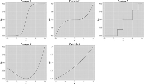
Table 1 reports the averaged MSPE ($\times 100$) and its standard error ($\times 100$) over 500 repetitions for methods in comparison. It is clear that the proposed methods with appropriate constraint have smaller MSPE than other methods in comparison. Note that it is important to impose appropriate constraint. In Example 4 which has a quadratic-shaped function, The performance of SCSS-Monotone is not as good as the SS since the monotone constraint is not proper here. When imposing the convexity constraint, the SCSS-convex performs much better than other methods. It is worth pointing out the B-spline method has comparable performance to the proposed method in Example 1, but not as good as the proposed method in other examples.

Table 1. Simulation studies comparing SCSS and other estimators under different functions and errors settings.Averaged MSPE ($\times 100$) and its standard error ($\times 100$) over 500 repetitions are reported. NA entries correspond to methods with no applicable settings.

						RS-		RS-		RS-		BS-		BS-		SCSS-		SCSS-		SCSS-
E.g.		Brunk's	(SE)	SS	(SE)	Monotone	(SE)	Convex	(SE)	Mixed	(SE)	Monotone	(SE)	Convex	(SE)	Monotone	(SE)	Convex	(SE)	Mixed	(SE)
1	normal	2.69	(0.08)	1.90	(0.05)	1.72	(0.05)	1.90	(0.05)	1.89	(0.04)	1.62	(0.02)	1.60	(0.02)	1.56	(0.05)	1.67	(0.07)	1.66	(0.08)
	t	2.75	(0.08)	1.96	(0.05)	1.74	(0.06)	1.91	(0.06)	1.89	(0.05)	1.61	(0.03)	1.60	(0.03)	1.66	(0.05)	1.74	(0.10)	1.73	(0.09)
	beta	2.87	(0.07)	1.97	(0.05)	1.72	(0.05)	1.89	(0.04)	1.89	(0.04)	1.62	(0.02)	1.61	(0.02)	1.67	(0.05)	1.69	(0.05)	1.67	(0.07)
2	normal	2.90	(0.07)	1.83	(0.05)	1.74	(0.05)	1.83	(0.05)	1.83	(0.05)	1.79	(0.03)	2.11	(0.06)	1.69	(0.05)	1.65	(0.06)	1.50	(0.05)
	t	3.07	(0.08)	1.84	(0.05)	1.74	(0.06)	1.83	(0.06)	1.83	(0.05)	1.79	(0.04)	2.11	(0.06)	1.71	(0.05)	1.69	(0.07)	1.51	(0.05)
	beta	2.91	(0.06)	1.88	(0.05)	1.74	(0.04)	1.83	(0.05)	1.83	(0.04)	1.79	(0.03)	2.12	(0.06)	1.71	(0.05)	1.72	(0.05)	1.53	(0.05)
3	normal	2.87	(0.07)	1.67	(0.04)	1.78	(0.05)	1.76	(0.05)	1.75	(0.04)	1.64	(0.02)	1.64	(0.02)	1.57	(0.03)	NA	(NA)	NA	(NA)
	t	2.86	(0.07)	1.71	(0.04)	1.79	(0.06)	1.77	(0.06)	1.75	(0.05)	1.64	(0.03)	1.64	(0.03)	1.62	(0.04)	NA	(NA)	NA	(NA)
	beta	2.85	(0.07)	1.70	(0.04)	1.78	(0.04)	1.76	(0.04)	1.75	(0.04)	1.64	(0.02)	1.64	(0.02)	1.63	(0.04)	NA	(NA)	NA	(NA)
4	normal	2.99	(0.07)	1.49	(0.06)	1.76	(0.04)	1.73	(0.05)	1.76	(0.04)	1.62	(0.02)	1.70	(0.02)	1.87	(0.04)	1.34	(0.05)	NA	(NA)
	t	2.95	(0.07)	1.49	(0.05)	1.77	(0.05)	1.74	(0.06)	1.76	(0.05)	1.62	(0.03)	1.70	(0.03)	1.86	(0.04)	1.34	(0.05)	NA	(NA)
	beta	2.97	(0.07)	1.47	(0.05)	1.76	(0.04)	1.73	(0.04)	1.76	(0.04)	1.62	(0.02)	1.70	(0.02)	1.91	(0.04)	1.42	(0.06)	NA	(NA)
5	normal	2.36	(0.06)	1.02	(0.04)	1.72	(0.04)	1.70	(0.05)	1.69	(0.04)	1.60	(0.02)	1.60	(0.02)	0.92	(0.03)	0.91	(0.08)	0.76	(0.03)
	t	2.39	(0.07)	1.00	(0.04)	1.73	(0.05)	1.71	(0.05)	1.70	(0.05)	1.60	(0.03)	1.60	(0.03)	0.92	(0.03)	0.88	(0.04)	0.74	(0.03)
	beta	2.25	(0.06)	0.98	(0.04)	1.72	(0.04)	1.70	(0.04)	1.69	(0.04)	1.60	(0.02)	1.60	(0.02)	0.88	(0.03)	0.87	(0.06)	0.82	(0.06)

Notes: Averaged MSPE ($\times 100$) and its standard error ($\times 100$) over 500 repetitions are reported. NA entries correspond to methods with no applicable settings.

Figure 5 to 10 in Appendix 3 report the estimator percentiles ($2.5\mathrm{\%}$ and $97.5\mathrm{\%}$) of SCSS and other estimators for Example 4 and Example 5. The SCSS-Monotone, SCSS-Convex and SCSS-Mixed produce slightly smoother percentile intervals compared to other methods, especially at the left and right boundaries on the x axis. Example 4 reveals the behaviour of SCSS under a mis-specified monotone constraint. On the interval $[-10,0]$, the true function in Example 4 is monotone decreasing but SCSS-Monotone is constrained to be non-decreasing.

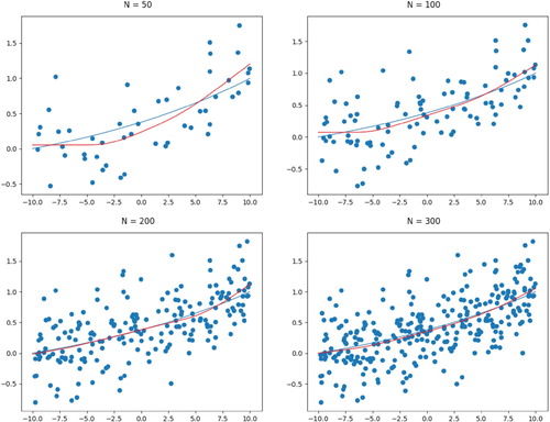
To further examine the rate of convergence, we consider a numerical study to check the proposed method's convergence as the sample size gets large. Taking Example 5 for elaboration, we allow the same size increasing gradually from $n=50$ to n = 300. At each given sample size, we compare the discrepancy between $f\left(x\right)$ and $\hat{f}\left(x\right)$ by $\int \left(f\right(x_i)-\hat{f}(x_i){)}^{2}dx$, Table 2 shows that as sample size increases, the function estimated by SCSS is getting closer to the true function. Figure 2 reports the convergence of the estimated function in Example 5 under the normal error and convex constraint. Results for the other two constraints can be found in the Appendix 3.

Figure 2. SCSS convergence for function $f\left(x\right)=\left(e^{x/20}-e^{-10/20}\right)/\left(e^{10/20}-e^{-10/20}\right)$ in Example 5 under normal error and convex constraint.

Table 2. Simulation studies measuring the convergence of SCSS based on the integrated mean squared errors.

E.g. 5		50	100	200	300
Normal	Monotone	6.81	5.82	2.44	2.29
	Convex	13.33	4.23	2.44	1.18
	Mixed	4.95	2.41	1.39	1.17

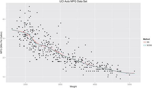
6. Real data analysis

In this section, we evaluate the performance of the proposed SCSS methods in comparison with the regular smoothing spline (SS). The Auto MPG Data from UCI Machine Learning Repository (Lichman, 2013) is used for our demonstration. This dataset concerning fuel consumption contains 398 observations with nine attributes: fuel consumption (miles per gallon), number of cylinders, engine displacement (cubic inches), horsepower, vehicle weight (pounds), time to accelerate from 0 to 60 mph (sec.), model year (modulo 100), origin of car (1. American, 2. European, 3. Japanese) and car names. For both methods, the optimal value of tuning parameter λ by minimising the average mean squared error from 10-fold cross-validation.

We first analyse relationship between the weight (weight) and the fuel consumption (mpg) of vehicles. Figure 3 confirms the intuition of a negative correlation between weight and mpg. Without any constraint, SS provided a monotone estimate that is consistent with the intuition. On the other hand, it is assuring to see that SCSS-Monotone provides an estimate that almost overlaps its unconstrained counterpart.

Figure 3. Comparison between unconstrained (SS) and monotone constrained (SCSS) smoothing spline for the Auto MPG Data. The response is mpg, modelled as a function of weight.

Next we consider the vehicle's volume (displacement) to be the predictor variable instead of weight. In general, one would expect a negative correlation between mpg and displacement. Figure 4 reveals the potential problem when prior knowledge on the function shape is not incorporated. The wiggly function estimated by SS contradicts the expectation of a monotone decreasing relationship between mpg and displacement. While the proposed SCSS-monotone capture the pattern of data quite well.

Figure 4. Comparison between unconstrained (SS) and monotone constrained (SCSS) smoothing spline for the Auto MPG Data. The response is mpg, modelled as a function of displacement.

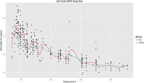
In a short summary, when one has prior shape information about the function to be estimated, it would be better to incorporate it into the estimation process. The proposed shape constraint smoothing spline can effectively help avoid unexpected results from non-parametric method.

7. Discussion

In this work, we proposed to impose the exact shape constraint on the smoothing spline, and enable efficient estimation. Compared to other methods also based on the fundamental assumption that the resulted function is a NCS with knots at all data points, the proposed SCSS method guarantees constraints to be followed exactly and also allows mixed and/or non-global constraints.

The technique developed in the SSCS method can be extended for the additive model, partially linear regression model, the non-parametric model with covaraites, etc. The theoretical investigation of the asymptotic convergence of SSCS can be quite challenging due to the exact (i.e. over an interval) constraint. Some theoretical results are available for functional ANOVA using spline with shape constraint at given finite locations (Dai & Chien, 2017). However, such results can not be easily extended to the smoothing spline with exact constraint. Another future study is to formulate necessary and sufficient conditions for function bound constraint and log-convexity constraint. In addition, efficient optimisation methods that take advantage of a quadratic program with non-linear constraints could be useful for further enhance our proposed method.

Disclosure statement

No potential conflict of interest was reported by the author(s).

Additional information

Funding

This work was supported by National Science Foundation [1634867].

Notes on contributors

Vincent Chan

Vincent Chan obtained his Ph.D. from the department of statistics at University of Wisconsin-Madison. His research interests include single index model and regularization.

Kam-Wah Tsui

Kam-Wah Tsui is a professor in the department of statistics at University of Wisconsin-Madison. His research interests include Bayesian analysis, decision theory, survey sampling, and statistical inference.

Yanran Wei

Yanran Wei is a Ph.D. student in the department of statistics at Virginia Tech. Her research interests include Big Data analytics, and statistical modeling in financial application.

Zhiyang Zhang

Zhiyang Zhang is a faculty in the department of statistics at Virginia Tech. Her research interests include modeling complex data, and statistical modeling in chemistry applications.

Xinwei Deng

Xinwei Deng is an associate professor in the department of statistics at Virginia Tech. His research interests include machine learning, design of experiment, and interface between machine learning and experimental design.

Appendices

Appendix 1

We provide some preliminary materials about natural cubic spline (NCS) and smoothing spline. Readers of interest can refer to Wahba (1990) and Green and Silverman (1993) for details.

A.1. Value-second derivative representation

The value-second derivative representation allows specification of a NCS simply by its value and second derivative at each knots. This representation provides a link between the entire NCS $f\left(x\right)$ and $(x_i,f(x_i\left)\right)$ for $i=1,\dots ,n$. Let us define $g_i=f\left(x_i\right)\mathrm{a}\mathrm{n}\mathrm{d}{\gamma }_i=f^{″}\left(x_i\right)\mathrm{f}\mathrm{o}\mathrm{r}i=1,\dots ,n.$ Also, let vector $\mathit{g}=(g_1,\dots ,g_n{)}^T$ and $\mathit{\gamma }=({\gamma }_1,\dots ,{\gamma }_n{)}^T$. Note that due to the natural boundary conditions of a NCS, ${\gamma }_1={\gamma }_n=0$. In addition, construct $n\times (n-2)$ matrix $\mathit{Q}$ and $(n-2)\times (n-2)$ matrix $\mathit{R}$ as follows: (A1) $\begin{array}{rl}\mathit{Q}& =\left(\begin{array}{ccc}{h}_1^{-1}& & \\ -h_1^{-1}-h_2^{-1}& \ddots & 0\\ h_2^{-1}& \ddots & \\ & \ddots & h_{n-2}^{-1}\\ 0& & -h_{n-2}^1-h_{n-1}^{-1}\\ & & h_{n-1}^{-1}\end{array}\right),\end{array}$(A1) (A2) $\begin{array}{rl}\mathit{R}& =\left(\begin{array}{cccc}\frac{1}{3}(h_1+h_2)& \frac{1}{6}{h}_2& & 0\\ \frac{1}{6}{h}_2& \ddots & \ddots & \\ & \ddots & \ddots & \frac{1}{6}{h}_{n-2}\\ 0& & \frac{1}{6}{h}_{n-2}& \frac{1}{3}(h_{n-2}+h_{n-1})\end{array}\right),\end{array}$(A2) where $h_i=x_{i+1}-x_i,\mathrm{f}\mathrm{o}\mathrm{r}i=1,\dots ,n-1$. By construction, matrix $\mathit{R}$ is strictly positive-definite.

Lemma A.1

Theorem 2.1 in Green and Silverman (1993)

The vectors $\mathit{g}$ and $\mathit{\gamma }$ specify a natural cubic spline f if and only if the condition (A3) ${\mathit{Q}}^T\mathit{g}=\mathit{R}\mathit{\gamma },$(A3) is satified. If (A3(A3) ${\mathit{Q}}^T\mathit{g}=\mathit{R}\mathit{\gamma },$(A3) ) is satified then the roughness penalty will satisfy (A4) $\int \left[f^{″}\right(t){]}^2\mathrm{d}t={\mathit{\gamma }}^T\mathit{R}\mathit{\gamma }={\mathit{g}}^T\mathit{K}\mathit{g},$(A4) where $\mathit{K}=\mathit{Q}{\mathit{R}}^{-1}{\mathit{Q}}^T$.

This value-second derivative representation provides a formula to recover the entire NCS with $x_i$ and $f\left(x_i\right)$ for $i=1,\dots ,n$.

A.2. Linear mixed model representation

The linear mixed model representation of an NCS allows us to express $f\left(x_1\right),\dots ,f\left(x_n\right)$ as a linear combination of a specific basis functions. Let function f be an NCS on interval $[a,b]$. Denote ${\mathcal{L}}^2[a,b]$ the space of square integrable functions on interval $[a,b]$. Let $\mathcal{H}=\{f:f,f^{\prime }$ are absolutely continuous, $f^{″}\in {\mathcal{L}}^2[a,b]\}$ be a second-order Sobolev space of the NCS functions. Under the following definition of norm $||f|{|}^2={\left[{\int }_a^{b}f\left(x\right)\mathrm{d}x\right]}^2+{\left[{\int }_a^b{f}^{\prime }\left(x\right)\mathrm{d}x\right]}^2+{\int }_a^b\left[f^{″}\right(x){]}^2\mathrm{d}x.$ Wahba (1990) shows that $\mathcal{H}$ is a reproducing kernel Hilbert space that can be decomposed into a direct sum of three orthogonal subspaces: $\mathcal{H}=\left\{1\right\}\oplus {\mathcal{H}}_0\oplus {\mathcal{H}}_1,$ where $\left\{1\right\}$ is the mean subspace, ${\mathcal{H}}_0=\{f:f^{″}(x)=0\}$ is the linear contrast subspace and ${\mathcal{H}}_1=\{f:{\int }_a^{b}f(x)dx=0,{\int }_a^b{f}^{\prime }(x)dx=0,{\int }_a^b{f}^{″}(x)dx\in \mathcal{L}[a,b\left]\right\}$ is the non-linear subspace. This decomposition means that any NCS function $f\in \mathcal{H}$ can be uniquely decomposed into a sum of a constant part, a linear part and a non-linear part as follows: (A5) $f\left(x\right)={\theta }_0+x{\theta }_1+f_1\left(x\right),$(A5) for some functions $f_1\in {\mathcal{H}}_1$.

Knowing that the solution is necessarily a NCS with knots at $x_1,\dots ,x_n$, one particular form of Equation (A5(A5) $f\left(x\right)={\theta }_0+x{\theta }_1+f_1\left(x\right),$(A5) ) is given by the linear mixed model representation (Green 1987; Zhang et al. 1998) as follows: (A6) $\mathit{g}={\mathbf{1}}_n{\theta }_0+\mathit{x}{\theta }_1+\mathit{A}\text{β},$(A6) where $\mathit{A}=\mathit{Q}({\mathit{Q}}^T\mathit{Q}{)}^{-1}{\mathit{R}}^{1/2}$ is a $n\times (n-2)$ matrix, ${\mathbf{1}}_n$ is a length-n vector of ones and $\mathit{x}=(x_1,\dots ,x_n{)}^T$.

Appendix 2

The linear mixed model representation is used for efficient computation of NCS. Meanwhile, the piecewise polynomial representation is used for formulating shape constraint on NCS for the same problem. The connection between linear mixed model representation and piecewise polynomial representation are stated as follows.

A.3. Specifying the NCS function f from $\mathit{x}$ and $\mathit{g}$

Given $\mathit{x}$, matrice $\mathit{Q}$ and $\mathit{R}$ can be constructed as shown in Appendix A.2. The second derivative vector $\mathit{\gamma }$, can be obtained by Theorem A.1 as follows, (A7) $\mathit{\gamma }={\mathit{R}}^{-1}{\mathit{Q}}^T\mathit{g},$(A7) since $\mathit{R}$ is of full rank by construction. From Section 2.4.1 in Green and Silverman (1993), the derivate of $f(.)$ at knot $x_1$ and $x_n$ are $\begin{array}{rl}{g}_1^{\prime }& =\frac{g_2-g_1}{x_2-x_1}-\frac{1}{6}(x_2-x_1){\gamma }_2\\ g_n^{\prime }& =\frac{g_n-g_{n-1}}{x_n-x_{n-1}}+\frac{1}{6}(x_n-x_{n-1}){\gamma }_{n-1},\end{array}$ respectively. Finally, with $h_i=x_{i+1}-x_i$, the following formula summarised from Section 2.4.2 in Green and Silverman (1993) gives the entire NCS function f: $f\left(t\right)=\left\{\begin{array}{ll}{g}_1-(x_1-t)g_1^{\prime },& \mathrm{i}\mathrm{f}t\le x_1,\\ \frac{(t-x_i)g_{i+1}+(x_{i+1}-t)g_i}{h_i}\\ -\frac{(t-x_i)(x_{i+1}-t)}{6}\\ \left\{\left(1+\frac{t-x_i}{h_i}\right){\gamma }_{i+1}\right.\\ +\left.\left(1+\frac{x_{i+1}-t}{h_i}\right){\gamma }_i\right\},& \mathrm{i}\mathrm{f}{x}_i<t<x_{i+1}\\ & \mathrm{f}\mathrm{o}\mathrm{r}i\in (1,\dots ,n-1),\\ g_n+(t-x_n)g_n^{\prime },& \mathrm{i}\mathrm{f}t>x_n.\end{array}\right.$ Hence the NCS function f is fully specified. That is, we can reconstruct NCS function f from $\mathit{x}$ and $\mathit{g}$.

A.4. Specifying the piecewise polynomial representation given f

The resulting function f can be used to estimate all coefficients $a_i$, $b_i$, $c_i$ and $d_i$ under the piecewise polynomial representation of f. The steps are as follows:

1. Given $\mathit{x}$ and the function of f, get $\mathit{\gamma }$ from (A7(A7) $\mathit{\gamma }={\mathit{R}}^{-1}{\mathit{Q}}^T\mathit{g},$(A7) ).

2. Calculate $\left(f^{\prime }\right(x_1),\dots ,f^{\prime }(x_n){)}^T$ by Equation (2.20) and (2.21) in Green and Silverman (1993) as: $\begin{array}{rl}{f}^{\prime }\left(x_i\right)& =\frac{g_{i+1}-g_i}{x_{i+1}-x_i}\\ & -\frac{(x_{i+1}-x_i)(2{\gamma }_i+{\gamma }_{i+1})}{6},i=1,\dots ,n-1;\\ f^{\prime }\left(x_n\right)& =\frac{g_n-g_{n-1}}{x_n-x_{n-1}}+\frac{{\gamma }_{n-1}(x_n-x_{n-1})}{6}.\end{array}$

3. Obtain $c_0=f_0^{\prime }\left(x_1\right)$ and $c_n=f_n^{\prime }\left(x_n\right)$ based on the piecewise polynomial representation.

4. Using the fact $f^{″}\left(x_{i+1}\right)=6a_i{x}_{i+1}+2b_i$ and $f^{″}\left(x_i\right)=6a_i{x}_i+2b_i$, we get $a_i=\frac{1}{6}\left(\right({\gamma }_{i+1}-{\gamma }_i\left)/\right(x_{i+1}-x_i\left)\right)$ for $i=1,\dots ,n-1$.

5. With $a_i$'s from previous step, obtain $b_i=\frac{1}{2}({\gamma }_i-6a_i{x}_i)$ for $i=1,\dots ,n-1$.

6. From previous steps with $a_i$, $b_i$ and $f^{\prime }\left(x_i\right)$, obtain $c_i=f^{\prime }\left(x_i\right)-3a_i{x}_i^2-2b_i{x}_i$ for $i=1,\dots ,n-1$.

7. Obtain $d_n=f\left(x_n\right)-c_n{x}_n$, $d_0=f\left(x_1\right)-c_0{x}_1$, and $d_i=f\left(x_i\right)-a_i{x}_i^3-b_i{x}_i^2-c_i{x}_i$ for $i=1,\dots ,n-1$.

Appendix 3

Figure A1. The estimator percentiles ($2.5\mathrm{\%}$ and $97.5\mathrm{\%}$) of SCSS for function $f\left(x\right)=\left(20x^2+x^3\right)/3000$ in Example 4 under normal error.

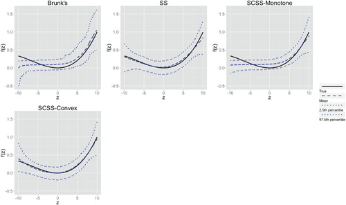
Figure A2. The estimator percentiles ($2.5\mathrm{\%}$ and $97.5\mathrm{\%}$) of SCSS for function $f\left(x\right)=\left(20x^2+x^3\right)/3000$ in Example 4 under t error.

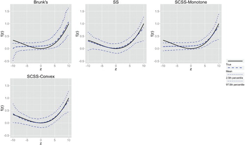
Figure A3. The estimator percentiles ($2.5\mathrm{\%}$ and $97.5\mathrm{\%}$) of SCSS for function $f\left(x\right)=\left(20x^2+x^3\right)/3000$ in Example 4 under beta error.

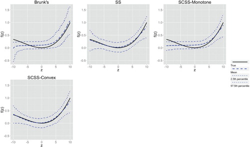
Figure A4. The estimator percentiles ($2.5\mathrm{\%}$ and $97.5\mathrm{\%}$) of SCSS for function $f\left(x\right)=\left(e^{x/20}-e^{-10/20}\right)/\left(e^{10/20}-e^{-10/20}\right)$ in Example 5 under normal error.

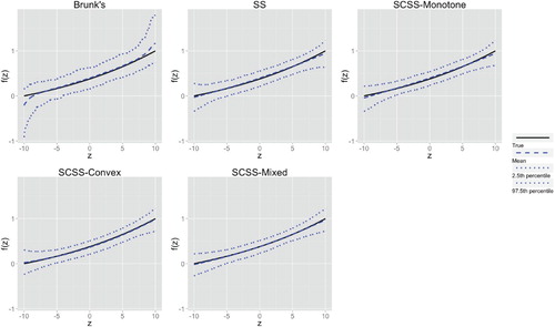
Figure A5. The estimator percentiles ($2.5\mathrm{\%}$ and $97.5\mathrm{\%}$) of SCSS for function $f\left(x\right)=\left(e^{x/20}-e^{-10/20}\right)/\left(e^{10/20}-e^{-10/20}\right)$ in Example 5 under t error.

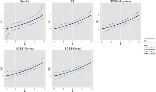
Figure A6. The estimator percentiles ($2.5\mathrm{\%}$ and $97.5\mathrm{\%}$) of SCSS for function $f\left(x\right)=\left(e^{x/20}-e^{-10/20}\right)/\left(e^{10/20}-e^{-10/20}\right)$ in Example 5 under beta error.

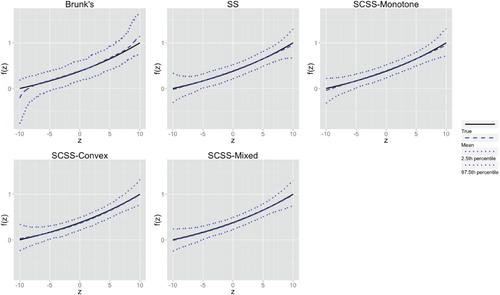
Figure A7. SCSS convergence for function $f\left(x\right)=\left(e^{x/20}-e^{-10/20}\right)/\left(e^{10/20}-e^{-10/20}\right)$ in Example 5 under normal error and monotone constraint.

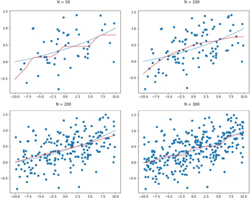
Figure A8. SCSS convergence for function $f\left(x\right)=\left(e^{x/20}-e^{-10/20}\right)/\left(e^{10/20}-e^{-10/20}\right)$ in Example 5 under normal error and mixed constraint.

References

- Brezger, A., & Steiner, W. J. (2003). Monotonic regression based on Bayesian P-splines: An application to estimating price response functions from store-level scanner data. Tech. rep., Discussion paper//Sonderforschungsbereich 386 der Ludwig-Maximilians-Universität München.
- Curry, H. B., & Schoenberg, I. J. (1966). On Pólya frequency functions IV: The fundamental spline functions and their limits. Journal D'analyse Mathématique, 17, 71–107. doi: 10.1007/BF02788653
- Dai, X., & Chien, P. (2017). Minimax optimal rates of estimation in functional anova models with derivatives. arXiv:1706.00850.
- Delecroix, M., & Thomas-Agnan, C. (2000). Spline and Kernel regression under shape restrictions. In Smoothing and Regression: Approaches, Computation, and Application (pp. 109–133).
- Dierckx, I. P (1980). Algorithm/algorithmus 42 an algorithm for cubic spline fitting with convexity constraints. Computing, 24, 349–371. doi: 10.1007/BF02237820
- Ducharme, G. R., & Fontez, B. (2004). A smooth test of goodness-of-fit for growth curves and monotonic nonlinear regression models. Biometrics, 60, 977–986. doi: 10.1111/j.0006-341X.2004.00253.x
- Fan, J., & Gijbels, I. (1996). Local polynomial modelling and its applications: Monographs on statistics and applied probability. New York: CRC Press.
- Green, P. J. (1987). Penalized likelihood for general semi-parametric regression models. International Statistical Review / Revue Internationale de Statistique, 55(3), 245.
- Green, P. J., & Silverman, B. W. (1993). Nonparametric regression and generalized linear models: A roughness penalty approach. New York: CRC Press.
- Hastie, T., Tibshirani, R., & Friedman, J, The elements of statistical learning, Springer series in statistics Springer (Vol. 1). Berlin, 2001.
- He, X., & Shi, P. (1998). Monotone B-spline smoothing. Journal of the American Statistical Association, 93, 643–650.
- Kelly, C., & Rice, J. (1990). Monotone smoothing with application to dose-response curves and the assessment of synergism. Biometrics, 46(4), 1071–1085. doi: 10.2307/2532449
- Liao, X., & Meyer, M. C. (2017). Change-point estimation using shape-restricted regression splines. Journal of Statistical Planning and Inference, 188, 8–21. doi: 10.1016/j.jspi.2017.03.007
- Lichman, M. (2013), UCI machine learning repository.
- Mammen, E., & Thomas-Agnan, C. (1999). Smoothing splines and shape restrictions. Scandinavian Journal of Statistics, 26, 239–252. doi: 10.1111/1467-9469.00147
- Matzkin, R. L. (1991). Semiparametric estimation of monotone and concave utility functions for polychotomous choice models. Econometrica: Journal of the Econometric Society, 59,1315–1327. doi: 10.2307/2938369
- Meyer, M. C. (2008). Inference using shape-restricted regression splines. The Annals of Applied Statistics, 2, 1013–1033. doi: 10.1214/08-AOAS167
- Meyer, M. C. (2012). Constrained penalized splines. Canadian Journal of Statistics, 40, 190–206. doi: 10.1002/cjs.10137
- Meyer, M. C. (2018). Constrained partial linear regression splines. Statistica Sinica, 28, 277–292.
- Nagahara, M., & Martin, C. F. (2013). Monotone smoothing splines using general linear systems. Asian Journal of Control, 15, 461–468. doi: 10.1002/asjc.557
- Ramsay, J. O. (1988). Monotone regression splines in action. Statistical Science, 3,425–441. doi: 10.1214/ss/1177012761
- Shor, N. Z., & Zhurbenko, N. (1971). The minimization method using space dilatation in direction of difference of two sequential gradients. Kibernetika, 3, 51–59.
- Turlach, B. A. (2005). Shape constrained smoothing using smoothing splines. Computational Statistics, 20, 81–104. doi: 10.1007/BF02736124
- Utreras, F. I. (1985). Smoothing noisy data under monotonicity constraints existence, characterization and convergence rates. Numerische Mathematik, 47, 611–625. doi: 10.1007/BF01389460
- Villalobos, M., & Wahba, G. (1987). Inequality-constrained multivariate smoothing splines with application to the estimation of posterior probabilities. Journal of the American Statistical Association, 82, 239–248. doi: 10.1080/01621459.1987.10478426
- Wahba, G. (1990). Spline models for observational data. Philadelphia, Pennsylvania: Siam.
- Wand, M., & Jones, M.. (1995), Kernel smoothing. Vol. 60 of Monographs on statistics and applied probability.
- Wand, M. P., & Ormerod, J. T. (2008). On Semiparametric regression with O'sullivan penalized splines. Australian & New Zealand Journal of Statistics, 50(2), 179–198. doi: 10.1111/j.1467-842X.2008.00507.x
- Wang, X., & Li, F. (2008). Isotonic smoothing spline regression. Journal of Computational and Graphical Statistics, 17, 21–37. doi: 10.1198/106186008X285627
- Zeng, L., Deng, X., & Yang, J. (2016). Constrained hierarchical modeling of degradation data in tissue-engineered scaffold fabrication. IIE Transactions, 48, 16–33. doi: 10.1080/0740817X.2015.1019164
- Zhang, D., Lin, X., Raz, J., & Sowers, M. (1998). Semiparametric stochastic mixed models for longitudinal data. Journal of the American Statistical Association, 93(442), 710. doi: 10.1080/01621459.1998.10473723