β-divergence loss for the kernel density estimation with bias reduced

Abstract

In this paper, we investigate the problem of estimating the probability density function. The kernel density estimation with bias reduced is nowadays a standard technique in explorative data analysis, there is still a big dispute on how to assess the quality of the estimate and which choice of bandwidth is optimal. This framework examines the most important bandwidth selection methods for kernel density estimation in the context of with bias reduction. Normal reference, least squares cross-validation, biased cross-validation and β-divergence loss methods are described and expressions are presented. In order to assess the performance of our various bandwidth selectors, numerical simulations and environmental data are carried out.

Keywords:

• bandwidth
• β-divergence
• nonparametric estimation
• bias reduction
• environmental data

1. Introduction

Selecting an appropriate bandwidth for a kernel density estimator is of crucial importance, and the purpose of the estimation may be an influential factor in the selection method. In many situations, it is sufficient to subjectively choose the smoothing parameter by looking at the density estimates produced by a range of bandwidths. A good overview on kernel density estimators is supplied by Silverman (1986), Scott (1992), Mugdadi and Ibrahim (2004). Let $(X_1,\dots ,X_n)$ be a sample of size n identically distributed with unknown probability density function (p.d.f) f. The kernel density estimator was introduced by Parzen (1962). Let K be a kernel function on real line, and let h be a positive value called bandwidth. Then kernel density estimator of f is defined as (1) $f_{n,h}\left(x\right)=\frac{1}{nh}\sum _{i=1}^{n}K\left(\frac{x-X_i}{h}\right).$(1)

To make the estimator meaningful, the kernel function is usually required to satisfy conditions $K\left(x\right)>0$, $\int K\left(x\right)\text{d}x=1$, $\int xK\left(x\right)\text{d}x=0$ and $\int x^{2}K\left(x\right)\text{d}x<\mathrm{\infty }$. Note that the bandwidth $h:=h_n\downarrow 0$, as $n\uparrow \mathrm{\infty }$. The choice of this bandwidth is very important. Several approaches are known for the choice of bandwidth in the kernel smoothing methods, via cross validation or by minimising a measure of error.

Studies are shown that the kernel density estimation of f in (1(1) $f_{n,h}\left(x\right)=\frac{1}{nh}\sum _{i=1}^{n}K\left(\frac{x-X_i}{h}\right).$(1) ) is biased. Recently, Xie and Wu (2014) studied a bias reduced version of $f_n$ and proved its performances comparing it to the usual methods. If the density f is twice continuously differentiable, this bias reduced estimator is given as follows (2) $\begin{array}{rl}{\hat{f}}_{n,h}\left(x\right)& =f_{n,h}\left(x\right)-\widehat{\text{Bias}}\left(f_{n,h}\right(x\left)\right),\\ & =f_{n,h}\left(x\right)-\frac{h^2}{2}{f}_n^{″}\left(x\right)\int t^{2}K\left(t\right)\text{d}t.\end{array}$(2) The bandwidth h is the most dominant parameter in the kernel density estimator. This parameter controls the amount of smoothing and is analogous to the bandwidth in a histogram. Even though the kernel estimator depends on the kernel and the bandwidth in a rather complicated way, a graphical representation clearly illustrates the difference in importance between these two parameters, see Figure 3.3 and 2.6(a) in Wand and Jones (1995). To explore the most relevant bandwidth selection methods in density estimation for complete data see the reviews of Turlach (1993), Cao et al. (1994), Jones et al. (1996) or Mammen et al. (2011) and Mammen et al. (2014), and the recent work on β-divergence for Bandwidth Selection by Dhaker et al. (2018).

It should be noticed that nonparametric estimation procedures have been recently applied in environmental data, e.g., Schmalensee et al. (1998), Taskin and Zaim (2000), Millimet and Stengos (2000), and Millimet et al. (2003). However, the nonparametric modelling used in this paper is for another purpose which is to study the dynamics of the entire distribution of CO₂ emissions per capita.

Our aim in this paper is to propose and compare several bandwidth selection procedures for the kernel density estimator in (2(2) $\begin{array}{rl}{\hat{f}}_{n,h}\left(x\right)& =f_{n,h}\left(x\right)-\widehat{\text{Bias}}\left(f_{n,h}\right(x\left)\right),\\ & =f_{n,h}\left(x\right)-\frac{h^2}{2}{f}_n^{″}\left(x\right)\int t^{2}K\left(t\right)\text{d}t.\end{array}$(2) ). The procedures we study are bandwidth selector based on the criterion of β-divergence with different β values. A simulation study is then carried out to assess the finite sample behaviour of these bandwidth selectors.

The remainder of the paper is organised as follows. In Section 2, we state our main results which presents the proposal method for bandwidth selector based on β-divergence $D_{\text{β}}$. Section 3 gives the estimation of the optimal bandwidth selection. Section 4 is devoted to our simulation results, Section 5 applies the methods to real datasets and finally, we conclude the paper in Section 6.

2. Bandwidth selection based on β-divergence

The β-divergence (see, e.g., Basu et al., 1998; Cichocki et al., 2006; Eguchi & Kano, 2001) is a general framework of similarity measures induced from various statistical models, such as Poisson, Gamma, Gaussian, Inverse Gaussian and compound Poisson distribution. For the connection between the β-divergence and various statistical distributions, see Jorgensen (1997). Beta divergence was proposed in Basu et al. (1998) and Minami and Eguchi (2002) and is defined as dissimilarity between the density function and its estimator as $\begin{array}{rl}{D}_{\text{β}}({\hat{f}}_{n,h},f)& =\frac{1}{\text{β}}\int {\left({\hat{f}}_{n,h}\left(x\right)\right)}^{\text{β}}\text{d}x-\frac{1}{\text{β}-1}\\ & \times \int {\left({\hat{f}}_{n,h}\left(x\right)\right)}^{\text{β}-1}f\left(x\right)\text{d}x+\frac{1}{\text{β}(\text{β}-1)}\\ & \times \int {\left(f\left(x\right)\right)}^{\text{β}}\text{d}x.\end{array}$In the case where $\text{β}=2$, we have $2D_2({\hat{f}}_{n,h},f)=ISE\left({\hat{f}}_{n,h}\right)=\int {\left({\hat{f}}_{n,h}\left(x\right)-f\left(x\right)\right)}^2\text{d}x.$Before we start our results, we introduce the following assumptions on the probability density function f and on the kernel K:

(F1)	f is compactly supported on I.
(F2)	f is four times continuously differentiable on I.
(F3)	${\int }_I\left(f^{\left(4\right)}\right(x\left){)}^2\right(f\left(x\right){)}^{\text{β}-2}\text{d}x<\mathrm{\infty }$.

Proposition 2.1

Under assumptions $\left(F1\right)\text{--}\left(F3\right),$ the mean of $D_{\text{β}}({\hat{f}}_{n,h},f)$ is given by (3) $\begin{array}{rl}\mathbb{E}{D}_{\text{β}}({\hat{f}}_{n,h},f)& :=A\mathbb{E}{D}_{\text{β}}({\hat{f}}_{n,h},f)+O_p\left(n^{-c}\right)+O\left(h^6\right),\\ 0& <c<\frac{1}{8},\end{array}$(3) where $A\mathbb{E}{D}_{\text{β}}({\hat{f}}_{n,h},f)$ is the asymptotic mean of $D_{\text{β}}({\hat{f}}_{n,h},f)$ expressed as (4) $\begin{array}{rl}A\mathbb{E}{D}_{\text{β}}({\hat{f}}_{n,h},f)& =\frac{h^8}{2\times 576}{\left({\int }_I{t}^{4}K\left(t\right)\mathrm{d}t\right)}^2\\ & \times \int {\left(f\left(x\right)\right)}^{\text{β}-2}{\left(f^{\left(4\right)}\left(x\right)\right)}^2\mathrm{d}x\\ & +\frac{1}{2nh}{\int }_I{\left(K\left(t\right)\right)}^2\mathrm{d}t\int {\left(f\left(x\right)\right)}^{\text{β}-1}\mathrm{d}x.\end{array}$(4)

For the proof of the Proposition 2.1, see appendix in Section A. The following theorem allows us to give the analytical value of bandwidth which minimises the asymptotic mean of $D_{\text{β}}({\hat{f}}_{n,h},f)$.

Theorem 2.2

Assume that $\left(F1\right)\text{--}\left(F3\right)$ hold, then the bandwidth $h_{\mathbb{E}{D}_{\text{β}}}$ that minimises $A\mathbb{E}{D}_{\text{β}}({\hat{f}}_{n,h},f)$ is (5) $\begin{array}{rl}{h}_{\text{β}}& =h_{\mathbb{E}{D}_{\text{β}}}\\ & ={\left\{72\frac{\int {\left(K\left(t\right)\right)}^2\mathrm{d}t{\int }_I{\left(f\left(x\right)\right)}^{\text{β}-1}\mathrm{d}x}{{\left(\int t^{4}K\left(t\right)\mathrm{d}t\right)}^2{\int }_I{\left(f\left(x\right)\right)}^{\text{β}-2}{\left(f^{\left(4\right)}\left(x\right)\right)}^2\mathrm{d}x}\right\}}^{1/9}\\ & \times n^{-1/9}.\end{array}$(5)

The proof of Theorem 2.2 is derived from Proposition 2.1. From Theorem 2.2, we deduce the particular case where $\text{β}=2$ of optimal bandwidth selection.

Corollary 2.3

Assuming that the assumptions in Theorem 2.2 hold. Then, we have for $\text{β}=2$ $\begin{array}{rl}\mathbb{E}{D}_2({\hat{f}}_{n,h},f)& =\frac{1}{2}MISE\left({\hat{f}}_{n,h}\right),\\ A\mathbb{E}{D}_2({\hat{f}}_h,f)& =\frac{1}{2}AMISE\left({\hat{f}}_{n,h}\right),\end{array}$with $AMISE\left({\hat{f}}_{n,h}\right)$ is the asymptotic $MISE\left({\hat{f}}_{n,h}\right)=\mathbb{E}ISE\left({\hat{f}}_{n,h}\right),$ and its corresponding optimal bandwidth is (6) $h_{AMISE}:=h_2={\left\{\frac{9}{2}\frac{R\left(K\right)}{{\left({\mu }_4\left(K\right)\right)}^{2}R\left(f^{\left(4\right)}\right)}\right\}}^{1/9}{n}^{-1/9},$(6) where $R\left(g\right)=\int {\left(g\left(t\right)\right)}^2\mathrm{d}t\text{and}{\mu }_4\left(K\right)=\int x^{4}K\left(x\right)\mathrm{d}x.$

3. The choice of the bandwidth h

In this section, we describe bandwidth selection methods for the density estimator defined in (2(2) $\begin{array}{rl}{\hat{f}}_{n,h}\left(x\right)& =f_{n,h}\left(x\right)-\widehat{\text{Bias}}\left(f_{n,h}\right(x\left)\right),\\ & =f_{n,h}\left(x\right)-\frac{h^2}{2}{f}_n^{″}\left(x\right)\int t^{2}K\left(t\right)\text{d}t.\end{array}$(2) ). These methods are adapted to common automatic selectors for kernel density estimation. We propose two selection methods a Normal reference and the cross-validation method. The Normal reference bandwidth is based on estimating the infeasible optimal expression (6(6) $h_{AMISE}:=h_2={\left\{\frac{9}{2}\frac{R\left(K\right)}{{\left({\mu }_4\left(K\right)\right)}^{2}R\left(f^{\left(4\right)}\right)}\right\}}^{1/9}{n}^{-1/9},$(6) ), in which the unknown element is $R\left(f^{\left(4\right)}\right)$.

3.1. Rule-of-thumb for bandwidth selection

This method is based on the rule-of-thumb for complete data (see, e.g., Silverman, 1986). The idea is to assume that the underlying distribution is normal, $\mathcal{N}(\mu ,\sigma )$, and in this situation, we have

Proposition 3.1

If f is Normal density function with mean μ and variance ${\sigma }^2,$ then the asymptotically optimal bandwidth $h_{\text{β}}$ in (5(5) $\begin{array}{rl}{h}_{\text{β}}& =h_{\mathbb{E}{D}_{\text{β}}}\\ & ={\left\{72\frac{\int {\left(K\left(t\right)\right)}^2\mathrm{d}t{\int }_I{\left(f\left(x\right)\right)}^{\text{β}-1}\mathrm{d}x}{{\left(\int t^{4}K\left(t\right)\mathrm{d}t\right)}^2{\int }_I{\left(f\left(x\right)\right)}^{\text{β}-2}{\left(f^{\left(4\right)}\left(x\right)\right)}^2\mathrm{d}x}\right\}}^{1/9}\\ & \times n^{-1/9}.\end{array}$(5) ) becomes the normal reference bandwidth as (7) $\begin{array}{rl}{h}_{N{R}_{\text{β}}}& =\sigma {\left\{\sqrt{\frac{2}{\pi }}\frac{4{\text{β}}^4}{9{\text{β}}^4-36{\text{β}}^3+90{\text{β}}^2+270\text{β}+105}\right\}}^{1/9}\\ & \times n^{-1/9}.\end{array}$(7)

In the particular case where $\text{β}=2$, we have $h_{N{R}_2}=\sigma {\left\{\sqrt{\frac{2}{\pi }}\frac{64}{861}\right\}}^{1/9}{n}^{-1/9}.$The standard deviation σ can be estimated by the sample standard deviation (S) or by the standardised interquartile range $IQR/1.34$ for robustness against outliers $(1.34={\mathrm{\Phi }}^{-1}(3/4)-{\mathrm{\Phi }}^{-1}(1/4\left)\right)$, but a better rule of thumb (e.g., Silverman, 1986, pp. 45–47; Härdle, 1991, p. 91) is to use $\hat{\sigma }=min(S,\frac{IQR}{1.34}),$ and to define the following estimator of $h_{N{R}_{\text{β}}}$ as $\begin{array}{rl}{\hat{h}}_{N{R}_{\text{β}}}& =\hat{\sigma }{\left\{\sqrt{\frac{2}{\pi }}\frac{4{\text{β}}^4}{9{\text{β}}^4-36{\text{β}}^3+90{\text{β}}^2+270\text{β}+105}\right\}}^{1/9}\\ & \times n^{-1/9}.\end{array}$Proof: See Appendix.

3.2. Cross-Validation

The method previously defined is based on minimising estimations of the mean $\mathbb{E}{D}_{\text{β}}({\hat{f}}_{n,h},f)$, more precisely of the asymptotic mean $A\mathbb{E}{D}_{\text{β}}({\hat{f}}_{n,h},f)$. The least squares Cross-Validation is the most popular method and is related on the minimising procedure of the ISE (integrated squared error), i.e., the particular case of β-divergence with $\text{β}=2$ (see, e.g., Bowman (1984) and Rudemo (1982)). As a generalisation of the ISE, we introduce a β-Divergence Cross Validation ($D_{\text{β}}CV$) method. Recall that $\begin{array}{rl}{D}_{\text{β}}({\hat{f}}_{n,h},f)& =\frac{1}{\text{β}}\int {\hat{f}}_{n,h}^{\text{β}}\left(x\right)\text{d}x-\frac{1}{\text{β}-1}\int {\hat{f}}_{n,h}^{\text{β}-1}\left(x\right)\\ & \times f\left(x\right)\text{d}x+\frac{1}{\text{β}(\text{β}-1)}\int f^{\text{β}}\left(x\right)\text{d}x.\end{array}$Since $\frac{1}{\text{β}(\text{β}-1)}\int f^{\text{β}}\left(x\right)\text{d}x$ does not depend on h, our β-Divergence Cross Validation approach is based on the minimising procedure likes the ISE method, of the following loss function: $\begin{array}{rl}{L}_{\text{β}}\left(h\right)& =D_{\text{β}}({\hat{f}}_{n,h},f)-\frac{1}{\text{β}(\text{β}-1)}\int f^{\text{β}}\left(x\right)\text{d}x,\\ & =\frac{1}{\text{β}}\int {\hat{f}}_{n,h}^{\text{β}}\left(x\right)\text{d}x-\frac{1}{\text{β}-1}\int {\hat{f}}_{n,h}^{\text{β}-1}\left(x\right)f\left(x\right)\text{d}x,\\ & =\frac{1}{\text{β}}\int {\hat{f}}_{n,h}^{\text{β}}\left(x\right)\text{d}x-\frac{1}{\text{β}-1}\mathbb{E}\left({\hat{f}}_{n,h}^{\text{β}-1}\left(X\right)\right).\end{array}$Using the same methodology as the least squares cross-validation method we estimate $L_{\text{β}}\left(h\right)$ from the data and minimise it over h. Considering the following estimator of $L_{\text{β}}\left(h\right)$: $D_{\text{β}}CV\left(h\right)=\frac{1}{\text{β}}\int {\hat{f}}_{n,h}^{\text{β}}\left(x\right)\text{d}x-\frac{2}{n(\text{β}-1)}\sum _{i=1}^n{\hat{f}}_{n,h,-i}^{\text{β}-1}\left(X_i\right),$with ${\hat{f}}_{h,h,-i}\left(X_i\right)=\frac{1}{h(n-1)}\sum _{j\ne i}^{n}K\left(\frac{X_i-X_j}{h}\right).$Hence, the optimal bandwidth that minimises the estimator $D_{\text{β}}CV\left(h\right)$ is ${\hat{h}}_{D_{\text{β}}CV}=\arg \underset{h}{min}{D}_{\text{β}}CV\left(h\right).$

Remark 3.1

In the preceding section three bandwidths $h_{N{R}_{\text{β}}}$ and ${\hat{h}}_{D_{\text{β}}CV}$ were presented as possible optimal choices for density estimation. However, in practice none of them is known since they depend on the unknown parameter β. In the article Dhaker et al. (2018) the authors have shown that optimal β verifies: $1<\text{β}<2,$For a β value close to 1 we obtain optimal h obtained using the Kullback-Leibler criteria, and for beta close to 2 we obtain that of the mean integrated square error.

Remark 3.2

From Theorem 2.1 in Xie and Wu (2014), we have (8) $\begin{array}{rl}\mathrm{V}\mathrm{a}\mathrm{r}\left({\hat{f}}_{n,h}\right(x\left)\right)& =\frac{1}{nh}f\left(x\right){\left(\int u^{2}K\left(u\right)\text{d}u\right)}^2\\ & \times \int \left(K^{″}{)}^2\right(u)\text{d}u+O(n^{-1}),\end{array}$(8) this variance decreasing in h, while the optimal h for $f_{n,h}\left(x\right)$ is given by: $\hat{h}={\left\{\frac{\int \mathcal{K}\left(t{)}^2\text{d}t{\int }_{I}f\right(x{)}^{\text{β}-1}\text{d}x}{{\left[\int t^2\mathcal{K}\left(t\right)\text{d}t\right]}^2{\int }_{I}f\left(x{)}^{\text{β}-2}{f}^{\left(2\right)}\right(x{)}^2\text{d}x}\right\}}^{1/5}{n}^{-1/5},$more reference see Dhaker et al. (2018). The optimal $\hat{h}$ of the ordinary kernel estimator $f_{n,h}\left(x\right)$ is asymptotically inferior to the bias reduced kernel density estimator, ${\hat{f}}_{n,h}\left(x\right)$, since its convergence rate is $O\left(n^{-1/5}\right)$ compared to the bias reduced kernel density estimator's $O\left(n^{-1/9}\right)$ rate, which results in a decrease in variance (8(8) $\begin{array}{rl}\mathrm{V}\mathrm{a}\mathrm{r}\left({\hat{f}}_{n,h}\right(x\left)\right)& =\frac{1}{nh}f\left(x\right){\left(\int u^{2}K\left(u\right)\text{d}u\right)}^2\\ & \times \int \left(K^{″}{)}^2\right(u)\text{d}u+O(n^{-1}),\end{array}$(8) ).

4. Simulations

In this section, we evaluate the performance of the bandwidth selection procedures presented in Section 2. To this goal we have carried out a simulation study including rule-of-thumb (${\hat{h}}_{N{R}_2}$), the Least Squares Cross-Validation bandwidth (${\hat{h}}_{LSCV}:={\hat{h}}_{D_{2}CV}$) and the β-Divergence Cross Validation (${\hat{h}}_{D_{\text{β}}CV}$ with $\text{β}\in \{1.5,1.1,1.9\}$). Two simulation studies are carried out to evaluate different situations. First of all, as the population density, we used a normal mixture. In the second place, we used a lognormal mixture, who is a heavy-tailed distribution is subexponential.

4.1. Simulation study 1

For consideration of computation and generality, assume that the true density f is a normal mixture (9) $m(\mu ,{\sigma }^2)=0.5\mathcal{N}(0,1)+0.5\mathcal{N}(\mu ,{\sigma }^2),$(9) where $\mu \in \{0,1,5\}$ and $\sigma \in \{1,0.5,0.1\}$. One thousand Monte Carlo samples of size n are generated from the normal mixture model in Equation (9(9) $m(\mu ,{\sigma }^2)=0.5\mathcal{N}(0,1)+0.5\mathcal{N}(\mu ,{\sigma }^2),$(9) ) for each combination of $n\in \{50,200,700\}$. The results of our different sets of experiments are presented in Tables 1–3. The Table 1 gives the exhibits simulated relative efficiency $RE\left(\hat{h}\right)=MISE\left({\hat{f}}_{n,h_{MISE}}\right)/MISE\left({\hat{f}}_{n,\hat{h}}\right)$ of the kernel estimator, with $\hat{h}$ takes the bandwidth estimators ${\hat{h}}_{N{R}_2}$,${\hat{h}}_{LSCV}$ and ${\hat{h}}_{D_{\text{β}}CV}$, it is lower than 1, because the optimal bandwidth $h_{MISE}$ minimise MISE. Each bandwidth, mean $\mathbb{E}\left(\hat{h}\right)$ and mean relation error $\mathbb{E}(\hat{h}/h_{MISE}-1)$ are obtained, these values are given by respectively, Tables 2 and 1.

1. For all situations, each relative efficiency $RE\left(\hat{h}\right)<1$ because the optimal bandwidth $h_{MISE}$ minimises the MISE.

2. The normal reference bandwidth ${\hat{h}}_{N{R}_2}$ performs well if the true density is not very far from normal, such as the cases of $(\mu ,\sigma )\in \left\{\right(0,1),(0,0.5),(1,1),(1,0.5\left)\right\}$. Otherwise, it usually has the smallest $RE\left(\hat{h}\right)$ and largest $E\left(\hat{h}\right)$, tending to oversmooth its kernel density estimate the most.

3. We have to remark that in Table 1, ${\hat{h}}_{LSCV}$ needs a large sample size in order to be competitive. Note also that in Table 2, it is seen that $\mathbb{E}\left({\hat{h}}_{LSCV}\right)$ is close to the optimal $h_{MISE}$, but the corresponding $\mathbb{E}\left({\hat{h}}_{LSCV}/{\hat{h}}_{MISE}\right)$ is large, which means that the bias of ${\hat{h}}_{LSCV}$ is small but its variation is large in Table 3.

4. The bandwidth ${\hat{h}}_{D_{\text{β}}CV}$ seems to be the best existing bandwidth selectors. In most situations, it is indeed one of the best bandwidth selectors, However, it behaves very poorly for small σ (the true density curve is sharp).

Table 1. $RE\left(\hat{h}\right)$ for normal mixture $f\left(x\right)=0.5\varphi \left(x\right)+0.5{\varphi }_{\sigma }(x-\mu )$.

n	${\hat{h}}_{NR}$	${\hat{h}}_{LSCV}$	${\hat{h}}_{{\mathcal{D}}_{1.1}CV}$	${\hat{h}}_{{\mathcal{D}}_{1.5}CV}$	${\hat{h}}_{{\mathcal{D}}_{1.9}CV}$
		$\mu =0$	$\sigma =1$
50	0.934	0.953	0.853	0.723	0.703
200	0.945	0.925	0.955	0.931	0.903
700	0.990	0.945	0.982	0.987	0.952
		$\mu =0$	$\sigma =0.5$
50	0.870	0.837	0.867	0.890	0.905
200	0.937	0.880	0.897	0.954	0.932
700	0.964	0.930	0.929	0.842	0.858
		$\mu =0$	$\sigma =0.1$
50	0.584	0.767	0.634	0.631	0.623
200	0.553	0.892	0.625	0.879	0.721
700	0.529	0.946	0.612	0.877	0.813
		$\mu =1$	$\sigma =1$
50	0.864	0.899	0.904	0.853	0.876
200	0.938	0.928	0.914	0.962	0.987
700	0.973	0.952	0.974	0.927	0.932
		$\mu =1$	$\sigma =0.5$
50	0.882	0.852	0.823	0.734	0.872
200	0.963	0.880	0.780	0.925	0.967
700	0.836	0.925	0.743	0.943	0.780
		$\mu =1$	$\sigma =0.1$
50	0.230	0.770	0.611	0.587	0.554
200	0.101	0.912	0.686	0.769	0.687
700	0.051	0.949	0.727	0.880	0.721
		$\mu =5$	$\sigma =1$
50	0.400	0.810	0.723	0.889	0.457
200	0.285	0.945	0.852	0.934	0.579
700	0.222	0.963	0.967	0.978	0.789
		$\mu =5$	$\sigma =0.5$
50	0.2390	0.852	0.712	0.845	0.831
200	0.1390	0.926	0.897	0.915	0.805
700	0.0817	0.956	0.945	0.921	0.878
		$\mu =5$	$\sigma =0.1$
50	0.1360	0.588	0.702	0.645	0.613
200	0.0523	0.458	0.764	0.758	0.802
700	0.0205	0.341	0.861	0.655	0.841

Table 2. $E\left(\hat{h}\right)$ for normal mixture $f\left(x\right)=0.5\varphi \left(x\right)+0.5{\varphi }_{\sigma }(x-\mu )$.

n	${\hat{h}}_{NR}$	${\hat{h}}_{LSCV}$	${\hat{h}}_{{\mathcal{D}}_{1.1}CV}$	${\hat{h}}_{{\mathcal{D}}_{1.5}CV}$	${\hat{h}}_{{\mathcal{D}}_{1.9}CV}$	$h_{MISE}$
			$\mu =0$	$\sigma =1$
50	0.464	0.528	0.530	0.520	0.323	0.347
200	0.362	0.393	0.399	0.383	0.321	0.328
700	0.287	0.302	0.310	0.293	0.308	0.309
			$\mu =0$	$\sigma =0.5$
50	0.330	0.397	0.425	0.343	0.223	0.286
200	0.248	0.267	0.312	0.248	0.193	0.280
700	0.196	0.197	0.242	0.200	0.186	0.244
			$\mu =0$	$\sigma =0.1$
50	0.134	0.104	0.358	0.098	0.510	0.041
200	0.087	0.060	0.027	0.087	0.485	0.038
700	0.068	0.043	0.219	0.057	0.421	0.0370
			$\mu =1$	$\sigma =1$
50	0.520	0.590	0.592	0.588	0.429	0.426
200	0.404	0.437	0.444	0.434	0.395	0.423
700	0.316	0.336	0.344	0.333	0.354	0.345
			$\mu =1$	$\sigma =0.5$
50	0.401	0.430	0.479	0.373	0.326	0.342
200	0.320	0.298	0.373	0.265	0.280	0.282
700	0.254	0.214	0.287	0.212	0.233	0.239
			$\mu =1$	$\sigma =0.1$
50	0.366	0.103	0.464	0.203	0.0422	0.0451
200	0.276	0.061	0.342	0.053	0.0380	0.0380
700	0.221	0.0428	0.267	0.0426	0.0343	0.0314
			$\mu =5$	$\sigma =1$
50	1.290	0.770	1.400	0.608	0.420	0.475
200	0.989	0.477	0.1.070	0.441	0.330	0.470
700	0.768	0.353	0.829	0.336	0.442	0.272
			$\mu =5$	$\sigma =0.5$
50	1.270	0.468	1.370	0.369	0.310	0.295
200	0.961	0.297	1.040	0.262	0.210	0.286
700	0.750	0.208	0.810	0.197	0.209	0.270
			$\mu =5$	$\sigma =0.1$
50	1.270	0.0982	1.370	0.0745	0.045	0.0415
200	0.955	0.061	1.030	0.053	0.040	0.0385
700	0.745	0.0424	0.804	0.040	0.039	0.0339

Table 3. $E|\hat{h}/h_{MISE}-1|$ for normal mixture $f\left(x\right)=0.5\varphi \left(x\right)+0.5{\varphi }_{\sigma }(x-\mu )$.

n	${\hat{h}}_{NR}$	${\hat{h}}_{LSCV}$	${\hat{h}}_{{\mathcal{D}}_{1.1}CV}$	${\hat{h}}_{{\mathcal{D}}_{1.5}CV}$	${\hat{h}}_{{\mathcal{D}}_{1.9}CV}$
		$\mu =0$	$\sigma =1$
50	0.124	0.072	0.077	0.0874	0.379
200	0.0785	0.0829	0.1050	0.0578	0.1620
700	0.0396	0.0717	0.0572	0.0436	0.0509
		$\mu =0$	$\sigma =0.5$
50	0.1370	0.1510	0.1670	0.1510	0.4560
200	0.0655	0.1360	0.0882	0.1010	0.2490
700	0.0559	0.0729	0.0537	0.0818	0.0104
		$\mu =0$	$\sigma =0.1$
50	0.772	0.2530	0.3000	0.3990	0.4410
200	0.674	0.1210	0.1250	0.1520	0.2070
700	0.679	0.0772	0.0506	0.0726	0.185
		$\mu =1$	$\sigma =1$
50	0.1430	0.1040	0.1630	0.0748	0.398
200	0.0774	0.0800	0.0931	0.0501	0.184
700	0.0483	0.0626	0.0600	0.0361	0.037
		$\mu =1$	$\sigma =0.5$
50	0.172	0.1930	0.1400	0.2260	0.4560
200	0.236	0.1530	0.0899	0.1460	0.121
700	0.285	0.0989	0.0506	0.0794	0.119
		$\mu =1$	$\sigma =0.1$
50	3.67	0.2620	1.380	0.3980	0.431
200	4.29	0.1250	0.986	0.1720	0.353
700	4.58	0.0838	0.652	0.0878	0.137
		$\mu =5$	$\sigma =1$
50	1.14	0.1450	0.2390	0.2430	0.4580
200	1.23	0.0815	0.1210	0.0899	0.2530
700	1.29	0.0686	0.0745	0.0540	0.0203
		$\mu =5$	$\sigma =0.5$
50	2.40	0.1860	0.600	0.2510	0.4340
200	2.68	0.1180	0.444	0.1440	0.2020
700	2.80	0.0743	0.296	0.0804	0.0597
		$\mu =5$	$\sigma =0.1$
50	15.7	0.884	5.95	0.3980	0.4810
200	17.1	1.021	4.51	0.1570	0.2630
700	17.7	1.104	3.34	0.0656	0.0178

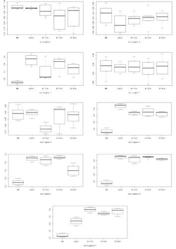
Figure 1 compare, for densities with $(\mu =0,1,5$ and $\sigma =1,0.5,0.1)$, the results of the five bandwidth selection ${\hat{h}}_{N{R}_2}$, ${\hat{h}}_{LSCV}$ and ${\hat{h}}_{D_{\text{β}}CV}$ (discussed in Section 3), relatively to the results obtained by using the MISE optimal bandwidth ($h_{MISE}$). These figures present boxplots of the ratio $RE\left(\hat{h}\right)=MISE\left({\hat{f}}_{n,h_{MISE}}\right)/MISE\left({\hat{f}}_{n,\hat{h}}\right)$, where $\hat{h}$ takes the estimators ${\hat{h}}_{N{R}_2}$, ${\hat{h}}_{LSCV}$ and ${\hat{h}}_{D_{\text{β}}CV}$, with $\text{β}=1.1,1.5,1.9$. We see the LSCV and $D_{\text{β}}CV$ (with $\text{β}=1.5$) methods gave overall the bests ratios across all simulations, and that this ratio was rather large in general.

Figure 1. Boxplots of the relative values RE for the bandwidth selectors for the estimation of densities $\mu =0,1,5$ and $\sigma =1,0.5,0.1$. The sample size varies from 100 to 2000.

4.2. Simulation study 2

As the populational density, we used a lognormal mixture. (10) $m(\mu ,{\sigma }^2)=0.5\log \mathcal{N}(0,1)+0.5\log \mathcal{N}(\mu ,{\sigma }^2),$(10) Where $\mu \in \{0,1,5\}$ and $\sigma \in \{1,0.5,0.1\}$, with μ and σ are the means and standard deviations, respectively. Similar to the previous subsection for each combination of n = 50, 200, 700, $\mu =0,1,5$, and $\rho =1,0.5,0.1$. For each case, Table 4 exhibits the simulated relative efficiency RE, Tables 5 and 6 give the $\mathbb{E}\left(\hat{h}\right)$ and $\mathbb{E}|\hat{h}/h_{MISE}-1|$ corresponding each bandwidth.

A summary of the results is provided below.

Firstly, in Table showed that the REs values for ${\hat{h}}_{NR}$ and ${\hat{h}}_{LSCV}$ increased as n increased and close to 1, but the performance is not so good in the case $(\mu ,\sigma )=\left\{\right(1,0.1),(5,1),(5,0.5),(5,0.1\left)\right\}$. However ${\hat{h}}_{{\mathcal{D}}_{\text{β}}CV}$ outperform others, especially ${\hat{h}}_{{\mathcal{D}}_{1.9}CV}$ which has RE values close to 1 in all situations.

Table 4. $RE\left(\hat{h}\right)$ for lognormal mixture $f\left(x\right)=0.5\varphi \left(x\right)+0.5{\varphi }_{\sigma }(x-\mu )$.

n	${\hat{h}}_{NR}$	${\hat{h}}_{LSCV}$	${\hat{h}}_{{\mathcal{D}}_{1.1}CV}$	${\hat{h}}_{{\mathcal{D}}_{1.5}CV}$	${\hat{h}}_{{\mathcal{D}}_{1.9}CV}$
		$\mu =0$	$\sigma =1$
50	0.901	0.933	0.905	0.920	0.923
200	0.949	0.972	0.949	0.935	0.956
700	0.969	0.987	0.978	0.988	0.990
		$\mu =0$	$\sigma =0.5$
50	0.880	0.883	0.856	0.885	0.890
200	0.938	0.844	0.886	0.887	0.893
700	0.962	0.817	0.942	0.943	0.950
		$\mu =0$	$\sigma =0.1$
50	0.627	0.218	0.798	0.699	0.802
200	0.561	0.096	0.830	0.708	0.825
700	0.517	0.046	0.947	0.789	0.889
		$\mu =1$	$\sigma =1$
50	0.824	0.937	0.911	0.941	0.950
200	0.973	0.971	0.967	0.977	0.980
700	0.978	0.986	0.971	0.983	0.989
		$\mu =1$	$\sigma =0.5$
50	0.907	0.836	0.838	0.840	0.876
200	0.906	0.784	0.882	0.887	0.902
700	0.831	0.687	0.919	0.887	0.908
		$\mu =1$	$\sigma =0.1$
50	0.248	0.199	0.796	0.799	0.800
200	0.097	0.082	0.885	0.803	0.810
700	0.048	0.038	0.950	0.932	0.940
		$\mu =5$	$\sigma =1$
50	0.395	0.351	0.824	0.813	0.835
200	0.239	0.244	0.942	0.860	0.899
700	0.221	0.179	0.968	0.907	0.934
		$\mu =5$	$\sigma =0.5$
50	0.234	0.214	0.872	0.863	0.881
200	0.128	0.113	0.924	0.896	0.905
700	0.082	0.071	0.952	0.911	0.972
		$\mu =5$	$\sigma =0.1$
50	0.139	0.137	0.785	0.753	0.823
200	0.051	0.050	0.811	0.748	0.873
700	0.022	0.021	0.850	0.750	0.902

Table 5. $E\left(\hat{h}\right)$ for lognormal mixture $f\left(x\right)=0.5\varphi \left(x\right)+0.5{\varphi }_{\sigma }(x-\mu )$.

n	${\hat{h}}_{NR}$	${\hat{h}}_{LSCV}$	${\hat{h}}_{{\mathcal{D}}_{1.1}CV}$	${\hat{h}}_{{\mathcal{D}}_{1.5}CV}$	${\hat{h}}_{{\mathcal{D}}_{1.9}CV}$	$h_{MISE}$
			$\mu =0$	$\sigma =1$
50	0.451	0.452	0.512	0.518	0.520	0.507
200	0.356	0.354	0.387	0.396	0.383	0.364
700	0.282	0.280	0.299	0.308	0.293	0.281
			$\mu =0$	$\sigma =0.5$
50	0.329	0.316	0.389	0.416	0.343	0.345
200	0.253	0.236	0.271	0.314	0.248	0.234
700	0.196	0.182	0.197	0.244	0.188	0.201
			$\mu =0$	$\sigma =0.1$
50	0.133	0.092	0.105	0.337	0.075	0.072
200	0.086	0.057	0.060	0.282	0.053	0.061
700	0.067	0.041	0.043	0.219	0.040	0.058
			$\mu =1$	$\sigma =1$
50	0.504	0.498	0.398	0.576	0.588	0.439
200	0.401	0.398	0.426	0.442	0.431	0.417
700	0.319	0.320	0.340	0.346	0.333	0.309
			$\mu =1$	$\sigma =0.5$
50	0.408	0.362	0.438	0.487	0.373	0.354
200	0.322	0.269	0.296	0.369	0.265	0.236
700	0.255	0.204	0.213	0.287	0.199	0.186
			$\mu =1$	$\sigma =0.1$
50	0.339	0.171	0.103	0.453	0.075	0.089
200	0.278	0.104	0.059	0.341	0.053	0.072
700	0.222	0.065	0.042	0.269	0.040	0.051
			$\mu =5$	$\sigma =1$
50	1.300	0.753	0.743	1.410	0.610	0.616
200	0.992	0.500	0.477	1.070	0.441	0.509
700	0.770	0.362	0.352	0.831	0.336	0.350
			$\mu =5$	$\sigma =0.5$
50	1.270	0.596	0.458	1.370	0.369	0.325
200	0.962	0.375	0.290	1.040	0.262	0.211
700	0.749	0.256	0.210	0.808	0.197	0.163
			$\mu =5$	$\sigma =0.1$
50	1.260	0.521	0.102	1.360	0.075	0.070
200	0.953	0.262	0.060	1.030	0.053	0.059
700	0.743	0.172	0.042	0.802	0.040	0.038

Table 6. $E|\hat{h}/h_{MISE}-1|$ for lognormal mixture $f\left(x\right)=0.5\varphi \left(x\right)+0.5{\varphi }_{\sigma }(x-\mu )$.

n	${\hat{h}}_{NR}$	${\hat{h}}_{LSCV}$	${\hat{h}}_{{\mathcal{D}}_{1.1}CV}$	${\hat{h}}_{{\mathcal{D}}_{1.5}CV}$	${\hat{h}}_{{\mathcal{D}}_{1.9}CV}$
		$\mu =0$	$\sigma =1$
50	0.143	0.165	0.090	0.081	0.078
200	0.079	0.102	0.056	0.051	0.049
700	0041.	0.065	0.045	0.050	0.046
		$\mu =0$	$\sigma =0.5$
50	0.133	0.167	0.175	0.221	0.207
200	0.067	0.095	0.122	0.268	0.202
700	0.052	0.062	0.071	0.295	0.195
		$\mu =0$	$\sigma =0.1$
50	0.777	0.307	409	4.010	0.532
200	0.629	0.109	0.153	4.320	0.321
700	678	0.058	0.087	4.511	0.029
		$\mu =1$	$\sigma =1$
50	0.156	0.178	0.097	0.088	0.076
200	0.078	0.109	0.050	0.041	0.039
700	0.043	0.054	0.041	0.036	0.
		$\mu =1$	$\sigma =0.5$
50	0.165	0.149	0.207	0.306	0.295
200	0.217	0.091	0.155	0.394	0.281
700	0.279	0.052	0.086	0.442	0.248
		$\mu =1$	$\sigma =0.1$
50	3.510	1.280	0.394	5.020	0.943
200	4.24	0.957	0.136	5.440	0.675
700	4.570	0.646	0.080	5.760	0.430
		$\mu =5$	$\sigma =1$
50	1.140	0.239	0.243	1.310	0.430
200	1.250	0.132	0.096	1.430	0.270
700	1.291	0.076	0.056	1.474	0.094
		$\mu =5$	$\sigma =0.5$
50	2.430	0.616	258	2.712	0.756
200	2.683	0.433	0.129	2.975	0.415
700	2.802	0.298	0.079	3.102	0.234
		$\mu =5$	$\sigma =0.1$
50	15.8	5.930	0.380	17.10	0.342
200	17.00	4.520	0.146	18.40	0.132
700	17.75	3.332	0.081	19.20	0.063

5. Real data analysis

A very natural use of density estimates is in the informal investigation of the properties of a given set of data. Density estimates can give valuable indication of such features as skewness, multimodality and heavy tail in the data. In some cases, they will yield conclusions that may then be regarded as self-evidently true, while in others all they will do is to point the way to further analysis and data collection.

Three examples of data are provided to illustrate the performance of kernel density estimation with different bandwidths, where the Gaussian kernel is used. All of them are classical examples of unimodal, bimodal distributions and heavy tail respectively.

5.1. Application 1

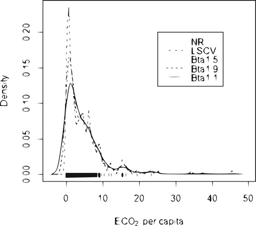
The first data set comprises the ${\text{CO}}_2$ per capita in the year of 2014. This data set is available in the world bank website. Figure 2 shows the estimated density of ${\text{CO}}_2$ per capita in the year of 2014 computing with bandwidths estimators ${\hat{h}}_{N{R}_2}=1.38$, ${\hat{h}}_{LSCV}=0.439$, ${\hat{h}}_{D_{1.5}CV}=0.832$, ${\hat{h}}_{D_{1.1}CV}=0.932$ and ${\hat{h}}_{D_{1.9}CV}=0.542$. The data set that the estimated density that was computed with the ${\hat{h}}_{LSCV}=0.439$ and ${\hat{h}}_{D_{1.9}CV}$ bandwidths captures the peak that characterises the mode, while the estimated density with the bandwidths that ${\hat{h}}_{N{R}_2}$, ${\hat{h}}_{D_{1.5}CV}$ and ${\hat{h}}_{D_{1.1}CV}$ smoothes out this peak. This happens because the outliers at the tail of the distribution contribute to ${\hat{h}}_{N{R}_2}$, ${\hat{h}}_{D_{1.5}CV}$ and ${\hat{h}}_{D_{1.1}CV}$ be larger than the other bandwidths.

Figure 2. Estimated density of $CO2$ per capita in 2008 using the different bandwidths. ${\hat{h}}_{D_{1.1}CV}$ (solid line); ${\hat{h}}_{D_{1.9}CV}$ (dashed line); ${\hat{h}}_{D_{1.5}CV}$ (dotted line); ${\hat{h}}_{LSCV}$, (dotdash line) and ${\hat{h}}_{N{R}_2}$ (longdash line).

5.2. Application 2

We use the time between eruptions set for the Old Faithful geyser in Yellowstone National Park, Wyoming, USA (107 sample data, source: Silverman, 1986). Figure 3 plots the data points and the kernel density estimates for old faithful geyser data, using bandwidths ${\hat{h}}_{NR}=0.442$, ${\hat{h}}_{LSCV}=0.162$, ${\hat{h}}_{D_{1.5}CV}=0.176$, ${\hat{h}}_{D_{1.1}CV}=0.281$ and ${\hat{h}}_{D_{1.9}CV}=0.210$.

Figure 3. Estimated density of repair times (hours) for an airborne communication transceiver: ${\hat{h}}_{D_{1.1}CV}$ (solid line); ${\hat{h}}_{D_{1.9}CV}$ (dashed line); ${\hat{h}}_{D_{1.5}CV}$ (dotted line); ${\hat{h}}_{LSCV}$, (dotdash line) and ${\hat{h}}_{N{R}_2}$, normal reference (longdash line).

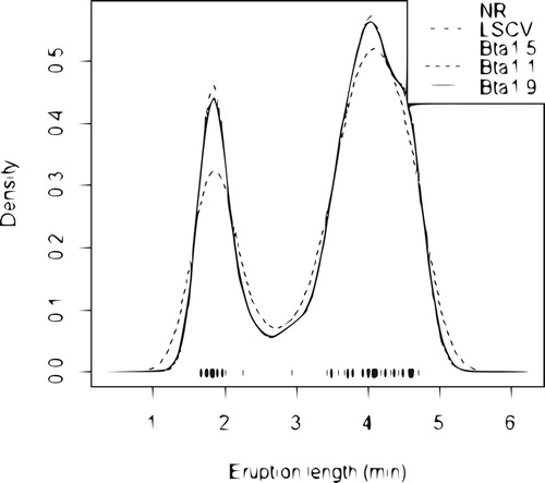
An important point to note that the density curve for eruption length is similar to bimodal normal density (normal mixture). From our Application 2, we see that the $h_{N{B}_2}$ is always larger than the others bandwidths, he heavily oversmoothes its kernel density curve, underestimating the two peaks of the curve but overestimating the valley between them. About $h_{LSCV}$, ${\hat{h}}_{D_{1.5}CV}$ and ${\hat{h}}_{D_{1.9}CV}$ seems to undersmooth the curve too much, overestimating the two peaks but underestimating for the valley. However ${\hat{h}}_{D_{1.1}CV}$ is proper bandwidth for their density estimate to be able to capture the feature of the true density curve.

5.3. Application 3

Maintenance data on 46 active repair times in hours for an airborne communication transceiver reported by Von Alven (1964) have been analysed by Sultan and Al-Moisheer (2015) who conclude that mixture of inverse Weibull and lognormal model was a good fit. The estimated density function of maintenance data is presented in Figure 4, using commonly used bandwidths ${\hat{h}}_{NR}=1.3150$, ${\hat{h}}_{LSCV}=0.5207$, as well as the newly developed bandwidth ${\hat{h}}_{D_{1.5}CV}=2.143$, ${\hat{h}}_{D_{1.1}CV}=2012$ and ${\hat{h}}_{D_{1.9}CV}=1859$.

Figure 4. Estimated density of repair times (hours) for an airborne communication transceiver using the different bandwidths: ${\hat{h}}_{D_{1.1}CV}$ (solid line); ${\hat{h}}_{D_{1.9}CV}$ (dashed line); ${\hat{h}}_{D_{1.5}CV}$ (dotted line); ${\hat{h}}_{LSCV}$, (dotdash line) and ${\hat{h}}_{N{R}_2}$, normal reference (longdash line).

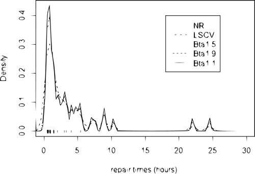
As expected, the normal reference bandwidth $h_{NR}$ heavily oversmoothes its kernel density curve. It seems that $h_{SJ}$ and $h_{LSCV4}$, especially the later, are appropriate bandwidths for their density estimates to be able to capture the feature of the true density curve.

As expected, the normal reference bandwidth $h_{NR}$ heavily oversmoothes its kernel density curve. It seems that ${\hat{h}}_{D_{1.9}CV}$ is appropriate bandwidth for their density estimate to be able to capture the feature of the true density curve.

6. Conclusion

This paper proposed the method for bandwidth selection of bias reduction kernel density estimator, given in (2(2) $\begin{array}{rl}{\hat{f}}_{n,h}\left(x\right)& =f_{n,h}\left(x\right)-\widehat{\text{Bias}}\left(f_{n,h}\right(x\left)\right),\\ & =f_{n,h}\left(x\right)-\frac{h^2}{2}{f}_n^{″}\left(x\right)\int t^{2}K\left(t\right)\text{d}t.\end{array}$(2) ). A various bandwidth selection strategies have been proposed such as normal reference ${\hat{h}}_{N{R}_2}$, least squares cross-validation ${\hat{h}}_{LSCV}$ and the β-Divergence Cross Validation ${\hat{h}}_{D_{\text{β}}CV}$, with $\text{β}=1.5,1.1$ and 1.9. The normal reference bandwidth method is a simple and quick selector, but limited the practical use, since they are restricted to situations where a pre-specified family of densities is correctly selected. The least squared cross validation method do not provide a smooth density estimation, although asymptotically optimal, the finite sample behaviour of ${\hat{h}}_{LSCV}$ is disappointing for its variability and undersmoothing. We have attempted to evaluate choice of the optimal bandwidth ${\hat{h}}_{LSCV}$ and ${\hat{h}}_{N{R}_2}$, using β-divergence. Compared to traditional bandwidth selection methods designed for kernel density estimation, our proposed ${\mathcal{D}}_{\text{β}}$ bandwidth selection method is always one of the best for having large $RE\left(\hat{h}\right)$ and small $\mathbb{E}(\hat{h}/h_{MISE}-1)$. Simulation studies showed that our proposed optimal bandwidth ${\mathcal{D}}_{\text{β}}$ method designed for kernel density estimation adapts to different situations, and out-performs other bandwidths. We conclude that the choice of the bandwidth based on the real data is consistent with the one based on simulations which is the ${\mathcal{D}}_{\text{β}}$ ($\text{β}=1.1$ and 1.5 ) method gives us a smoother density estimation.

Disclosure statement

No potential conflict of interest was reported by the author(s).

Additional information

Notes on contributors

Hamza Dhaker

Hamza Dhaker (PhD), is Assistant Professor in Probability and Statistic at the Faculty of Sciences of Université de Monctoon (Canada). His work revolves around Non-parametric Statistic, Extreme value statistic, Divergence Measures, Risk Measures.

El Hadji Deme

El Hadji Deme (PhD), is Associate Professor in Probablity and Statistic at the Faculty of Applied Sciences and Technology of Gaston Berger University in Saint-Louis (Senegal). His work revolves around Non-parametric Statistic, Extreme value statistic, Empirical process, Divergence Measures, Risk Measures (in finance and insurance), Inequality index and social well-being.

Youssou Ciss

Youssou Ciss (PhD) is Doctor of Applied Mathmatics Probabily and Statistics at the Faculty of Sciences and Technology in Gaston Berger University (Senegal). Field of work: Non parametric statistics.

Appendix

Proof of Proposition 2.1

${\hat{f}}_n^{\text{β}}\left(x\right)={\left(f_n\left(x\right)-\widehat{\mathrm{B}\mathrm{i}\mathrm{a}\mathrm{s}}\left(\hat{f}\right(x)\right)}^{\text{β}}.$

With a random variable $\xi =O_p\left(1\right)$ whose expectation is 0 and variance 1, we can write $f_n\left(x\right)$ as (see Kanazawa, 1993), (A1) $\begin{array}{rl}{f}_n\left(x\right)& =f\left(x\right)[1+\frac{h^2}{2}\frac{f^{\left(2\right)}\left(x\right)}{f\left(x\right)}{\int }_I{t}^2\mathcal{K}\left(t\right)\text{d}t+\frac{h^4}{24}\frac{f^{\left(4\right)}\left(x\right)}{f\left(x\right)}\\ & \times {\int }_I{t}^4\mathcal{K}\left(t\right)\text{d}t+O\left(h^6\right)\\ & +{\left\{\frac{{\int }_I\mathcal{K}(t{)}^2\text{d}t}{nhf\left(x\right)}\right\}}^{1/2}\xi +O_p\left(n^{-1/2}\right)].\end{array}$(A1)

Using the result of the Corollary 2.6 (Eugene, 1969), $\underset{n\to \mathrm{\infty }}{lim}\underset{x}{sup}{n}^c\left|f_n^{\left(r\right)}\right(x)-f^{\left(r\right)}(x\left)\right|=0\text{with}0<c<\frac{1}{2r+4},$we have, $\begin{array}{rl}{\hat{f}}_n\left(x\right)& =f_n\left(x\right)-\widehat{\mathrm{B}\mathrm{i}\mathrm{a}\mathrm{s}}\left(f_n\right(x\left)\right)=f_n\left(x\right)-\frac{h^2}{2}{f}_n^{\left(2\right)}{\int }_I{t}^2\mathcal{K}\left(t\right)\text{d}t\\ & =f_n\left(x\right)-\frac{h^2}{2}{f}^{\left(2\right)}{\int }_I{t}^2\mathcal{K}\left(t\right)\text{d}t+O\left(n^{-c}\right),\\ & =f\left(x\right)[1+\frac{h^2}{2}\frac{f^{\left(2\right)}\left(x\right)}{f\left(x\right)}{\int }_I{t}^2\mathcal{K}\left(t\right)\text{d}t+\frac{h^4}{24}\frac{f^{\left(4\right)}\left(x\right)}{f\left(x\right)}\\ & \times {\int }_I{t}^4\mathcal{K}\left(t\right)\text{d}t+O\left(h^6\right)+{\left\{\frac{{\int }_I\mathcal{K}(t{)}^2\text{d}t}{nhf\left(x\right)}\right\}}^{1/2}\xi \\ & +O_p\left(n^{-1/2}\right)]-\frac{h^2}{2}{f}^{\left(2\right)}{\int }_I{t}^{2}K\left(t\right)\text{d}t+O\left(n^{-c}\right),\\ & =f\left(x\right)[1+\frac{h^4}{24}\frac{f^{\left(4\right)}\left(x\right)}{f\left(x\right)}{\int }_I{t}^4\mathcal{K}\left(t\right)\text{d}t+O\left(h^6\right)\\ & +{\left\{\frac{{\int }_I\mathcal{K}(t{)}^2\text{d}t}{nhf\left(x\right)}\right\}}^{1/2}\xi +O_p\left(n^{-1/2}\right)+O\left(n^{-c}\right)].\end{array}$Where the $O\left(h^6\right)$ terms depend upon x. Using $(1+z{)}^{\text{β}}=1+\text{β}z+\frac{\text{β}(\text{β}-1)}{2}{z}^2+O(z^3)$,

$\begin{array}{rl}{\hat{f}}_n^{\text{β}}\left(x\right)& =f(x{)}^{\text{β}}[1+\frac{h^4}{24}\frac{f^{\left(4\right)}\left(x\right)}{f\left(x\right)}{\int }_I{t}^4\mathcal{K}(t)\text{d}t+O(h^6)\\ & +{\left\{\frac{{\int }_I\mathcal{K}(t{)}^2\text{d}t}{nhf\left(x\right)}\right\}}^{1/2}\xi +O_p\left(n^{-1/2}\right)+O\left(n^{-c}\right){]}^{\text{β}},\\ & =f(x{)}^{\text{β}}[1+\text{β}\left(\frac{h^4}{24}\frac{f^{\left(4\right)}\left(x\right)}{f\left(x\right)}{\int }_I{t}^4\mathcal{K}\left(t\right)\text{d}t+{\left\{\frac{{\int }_I\mathcal{K}(t{)}^2\text{d}t}{nhf\left(x\right)}\right\}}^{1/2}\xi \right)\\ & +\frac{\text{β}(\text{β}-1)}{2}\left(\frac{h^8}{576}\frac{\left(f^{\left(4\right)}\right(x){)}^2}{f^2\left(x\right)}{\left({\int }_I{t}^4\mathcal{K}\left(t\right)\text{d}t\right)}^2+\frac{{\int }_I\mathcal{K}(t{)}^2\text{d}t}{nhf\left(x\right)}{\xi }^2\right)\\ & +\phantom{\frac{\text{β}(\text{β}-1)}{2}\left(\frac{h^8}{576}\frac{\left(f^{\left(4\right)}\right(x){)}^2}{f^2\left(x\right)}\left({\int }_I{t}^4\mathcal{K}\right(t)\text{d}t{)}^2+\frac{{\int }_I\mathcal{K}(t{)}^2\text{d}t}{nhf\left(x\right)}{\xi }^2\right)}{O}_p\left(n^{-c}\right)+O\left(h^6\right)],\end{array}$and $\begin{array}{rl}{\hat{f}}_n^{\text{β}-1}\left(x\right)& =f(x{)}^{\text{β}-1}\left[1+\frac{h^4}{24}\frac{f^{\left(4\right)}\left(x\right)}{f\left(x\right)}{\int }_I{t}^4\mathcal{K}\left(t\right)\text{d}t+O\left(h^6\right)\right.\\ & {\left.+{\left\{\frac{{\int }_I\mathcal{K}(t{)}^2\text{d}t}{nhf\left(x\right)}\right\}}^{1/2}\xi +O_p\left(n^{-1/2}\right)+O\left(n^{-c}\right)\right]}^{\text{β}-1}\\ & =f(x{)}^{\text{β}-1}\left[1+(\text{β}-1)\left(\frac{h^4}{24}\frac{f^{\left(4\right)}\left(x\right)}{f\left(x\right)}{\int }_I{t}^4\mathcal{K}\left(t\right)\text{d}t\phantom{{\left\{\frac{{\int }_I\mathcal{K}(t{)}^2\text{d}t}{nhf\left(x\right)}\right\}}^{1/2}}\right.\right.\\ & \left.+{\left\{\frac{{\int }_I\mathcal{K}(t{)}^2\text{d}t}{nhf\left(x\right)}\right\}}^{1/2}\xi \right)+\frac{(\text{β}-1)(\text{β}-2)}{2}\\ & \times \left(\frac{h^8}{576}\frac{\left(f^{\left(4\right)}\right(x){)}^2}{f^2\left(x\right)}{\left({\int }_I{t}^4\mathcal{K}\left(t\right)\text{d}t\right)}^2+\frac{{\int }_I\mathcal{K}(t{)}^2\text{d}t}{nhf\left(x\right)}{\xi }^2\right)\\ & \left.\phantom{\left(\frac{h^8}{576}\frac{\left(f^{\left(4\right)}\right(x){)}^2}{f^2\left(x\right)}\left({\int }_I{t}^4\mathcal{K}\right(t)\text{d}t{)}^2+\frac{{\int }_I\mathcal{K}(t{)}^2\text{d}t}{nhf\left(x\right)}{\xi }^2\right)}+O_p\left(n^{-c}\right)+O\left(h^6\right)\right].\end{array}$ $\begin{array}{rl}& {\mathcal{D}}_{\text{β}}\left({\hat{f}}_n\right(x),f(x\left)\right)\\ & =\frac{1}{\text{β}}\int {\hat{f}}_n^{\text{β}}\left(x\right)\text{d}x-\frac{1}{\text{β}-1}\int {\hat{f}}_n^{\text{β}-1}\left(x\right)f\left(x\right)\text{d}x\\ & +\frac{1}{\text{β}(\text{β}-1)}\int f^{\text{β}}\left(x\right)\text{d}x,\\ & =\frac{1}{\text{β}}\int f(x{)}^{\text{β}}\left[1+\text{β}\left(\frac{h^4}{24}\frac{f^{\left(4\right)}\left(x\right)}{f\left(x\right)}{\int }_I{t}^4\mathcal{K}\left(t\right)\text{d}t\right.\right.\\ & \left.+{\left\{\frac{{\int }_I\mathcal{K}(t{)}^2\text{d}t}{nhf\left(x\right)}\right\}}^{1/2}\xi \right)\\ & +\frac{\text{β}(\text{β}-1)}{2}\left(\frac{h^8}{576}\frac{\left(f^{\left(4\right)}\right(x){)}^2}{f^2\left(x\right)}{\left({\int }_I{t}^4\mathcal{K}\left(t\right)\text{d}t\right)}^2\right.\\ & \left.\left.+\frac{{\int }_I\mathcal{K}(t{)}^2\text{d}t}{nhf\left(x\right)}{\xi }^2\right)+O_p\left(n^{-c}\right)+O\left(h^6\right)\right]\text{d}x\\ & -\frac{1}{\text{β}-1}\int f(x{)}^{\text{β}}\left[\phantom{\left.\left.+\frac{{\int }_I\mathcal{K}(t{)}^2\text{d}t}{nhf\left(x\right)}{\xi }^2\right)+O_p\left(n^{-c}\right)+O\left(h^6\right)\right]\text{d}x}1+(\text{β}-1)\right.\\ & \times \left(\frac{h^4}{24}\frac{f^{\left(4\right)}\left(x\right)}{f\left(x\right)}{\int }_I{t}^4\mathcal{K}\left(t\right)\text{d}t+{\left\{\frac{{\int }_I\mathcal{K}(t{)}^2\text{d}t}{nhf\left(x\right)}\right\}}^{1/2}\xi \right)\\ & +\frac{(\text{β}-1)(\text{β}-2)}{2}\\ & \times \left(\frac{h^8}{576}\frac{\left(f^{\left(4\right)}\right(x){)}^2}{f^2\left(x\right)}{\left({\int }_I{t}^4\mathcal{K}\left(t\right)\text{d}t\right)}^2+\frac{{\int }_I\mathcal{K}(t{)}^2\text{d}t}{nhf\left(x\right)}{\xi }^2\right)\\ & \left.\phantom{\left(\frac{h^8}{576}\frac{\left(f^{\left(4\right)}\right(x){)}^2}{f^2\left(x\right)}\left({\int }_I{t}^4\mathcal{K}\right(t)\text{d}t{)}^2+\frac{{\int }_I\mathcal{K}(t{)}^2\text{d}t}{nhf\left(x\right)}{\xi }^2\right)}+O_p\left(n^{-c}\right)+O\left(h^6\right)\right]\text{d}x+\frac{1}{\text{β}(\text{β}-1)}\int f^{\text{β}}\left(x\right)\text{d}x,\\ & =\frac{1}{\text{β}}\int f(x{)}^{\text{β}}\left[\frac{\text{β}(\text{β}-1)}{2}\left(\frac{h^8}{576}\frac{\left(f^{\left(4\right)}\right(x){)}^2}{f^2\left(x\right)}{\left({\int }_I{t}^4\mathcal{K}\left(t\right)\text{d}t\right)}^2\right.\right.\end{array}$ $\begin{array}{rl}& \left.+\frac{{\int }_I\mathcal{K}(t{)}^2\text{d}t}{nhf\left(x\right)}{\xi }^2\right)+O_p\left(n^{-c}\right)\\ & \left.\phantom{\left.+\frac{{\int }_I\mathcal{K}(t{)}^2\text{d}t}{nhf\left(x\right)}{\xi }^2\right)+O_p\left(n^{-c}\right)}+O\left(h^6\right)\right]\text{d}x-\frac{1}{\text{β}-1}\int f(x{)}^{\text{β}}\\ & \times \left[\frac{(\text{β}-1)(\text{β}-2)}{2}\left(\frac{h^8}{576}\frac{\left(f^{\left(4\right)}\right(x){)}^2}{f^2\left(x\right)}{\left({\int }_I{t}^4\mathcal{K}\left(t\right)\text{d}t\right)}^2\right.\right.\\ & \left.\left.+\frac{{\int }_I\mathcal{K}(t{)}^2\text{d}t}{nhf\left(x\right)}{\xi }^2\right)+O_p\left(n^{-c}\right)+O\left(h^6\right)\right]\text{d}x\\ & =\int f(x{)}^{\text{β}}\left[\left(\frac{\text{β}-1}{2}-\frac{\text{β}-2}{2}\right)\right.\\ & \times \left(\frac{h^8}{576}\frac{\left(f^{\left(4\right)}\right(x){)}^2}{f^2\left(x\right)}{\left({\int }_I{t}^4\mathcal{K}\left(t\right)\text{d}t\right)}^2+\frac{{\int }_I\mathcal{K}(t{)}^2\text{d}t}{nhf\left(x\right)}{\xi }^2\right)\\ & \left.\phantom{\left(\frac{h^8}{576}\frac{\left(f^{\left(4\right)}\right(x){)}^2}{f^2\left(x\right)}\left({\int }_I{t}^4\mathcal{K}\right(t)\text{d}t{)}^2+\frac{{\int }_I\mathcal{K}(t{)}^2\text{d}t}{nhf\left(x\right)}{\xi }^2\right)}+O_p\left(n^{-c}\right)+O\left(h^6\right)\right]\text{d}x\\ & =\frac{1}{2}\left[\frac{h^8}{576}{\left({\int }_I{t}^4\mathcal{K}\left(t\right)\text{d}t\right)}^2\int f^{\text{β}-2}\left(x\right){\left(f^{\left(4\right)}\right)}^2\left(x\right)\text{d}x\right.\\ & \left.+\frac{1}{nh}{\int }_I{\mathcal{K}}^2\left(t\right)\text{d}t\int f^{\text{β}-1}\left(x\right)\text{d}x{\xi }^2\right]\\ & +O_p\left(n^{-c}\right)+O\left(h^6\right),\\ & \mathbb{E}{\mathcal{D}}_{\text{β}}\left({\hat{f}}_n\right(x),f(x\left)\right)\\ & =\frac{1}{2}\left[\frac{h^8}{576}{\left({\int }_I{t}^4\mathcal{K}\left(t\right)\text{d}t\right)}^2\int f^{\text{β}-2}\left(x\right){\left(f^{\left(4\right)}\right)}^2\left(x\right)\text{d}x\right.\\ & \left.+\frac{1}{nh}{\int }_I{\mathcal{K}}^2\left(t\right)\text{d}t\int f^{\text{β}-1}\left(x\right)\text{d}x\right]\\ & +O_p\left(n^{-c}\right)+O\left(h^6\right).\end{array}$

Proof of Proposition 3.1

$f\left(x\right)=\frac{1}{\sigma \sqrt{2\pi }}{\mathrm{e}}^{-1/2(\frac{x-m}{\sigma }{)}^2},$so

$\begin{array}{rl}{f}^{\left(4\right)}\left(x\right)& =\frac{1}{{\sigma }^5\sqrt{2\pi }}{\mathrm{e}}^{-1/2(\frac{x-m}{\sigma }{)}^2}\\ & \times \left(3-6{\left(\frac{x-m}{\sigma }\right)}^2+{\left(\frac{x-m}{\sigma }\right)}^4\right),\\ {\left(f^{\left(4\right)}\left(x\right)\right)}^2& =\frac{1}{{\sigma }^{10}2\pi }{\mathrm{e}}^{-(\frac{x-m}{\sigma }{)}^2}\\ & \times \left(9-36{\left(\frac{x-m}{\sigma }\right)}^2+30{\left(\frac{x-m}{\sigma }\right)}^4\right.\\ & \left.+18{\left(\frac{x-m}{\sigma }\right)}^6+{\left(\frac{x-m}{\sigma }\right)}^8\right),\\ \int f^{\text{β}-2}\left(x\right){\left(f^{\left(4\right)}\left(x\right)\right)}^2\text{d}x& =\frac{1}{{\sigma }^{\text{β}+7}\sqrt{\text{β}}(2\pi {)}^{\frac{\text{β}-2}{2}}}\\ & \times \left(\frac{\begin{array}{c}9{\text{β}}^4-36{\text{β}}^3+90{\text{β}}^2+270\text{β}+105\end{array}}{{\text{β}}^4}\right).\end{array}$and $\int f^{\text{β}-1}\left(x\right)\text{d}x=\frac{1}{\sqrt{\text{β}-1}(2\pi {)}^{\frac{\text{β}-2}{2}}}.$

In that case the asymptotically optimal bandwidth $h_{\text{β}}$ in Equation (5(5) $\begin{array}{rl}{h}_{\text{β}}& =h_{\mathbb{E}{D}_{\text{β}}}\\ & ={\left\{72\frac{\int {\left(K\left(t\right)\right)}^2\mathrm{d}t{\int }_I{\left(f\left(x\right)\right)}^{\text{β}-1}\mathrm{d}x}{{\left(\int t^{4}K\left(t\right)\mathrm{d}t\right)}^2{\int }_I{\left(f\left(x\right)\right)}^{\text{β}-2}{\left(f^{\left(4\right)}\left(x\right)\right)}^2\mathrm{d}x}\right\}}^{1/9}\\ & \times n^{-1/9}.\end{array}$(5) ) becomes the normal reference bandwidth. $\begin{array}{rl}{h}_{\text{β}}& =h_{\mathbb{E}{\mathcal{D}}_{\text{β}}}={\left\{72\frac{R\left(\mathcal{K}\right){\int }_{I}f(x{)}^{\text{β}-1}\text{d}x}{{\mu }_4\left(\mathcal{K}{)}^2{\int }_{I}f\right(x{)}^{\text{β}-2}{\left(f^{\left(4\right)}\left(x\right)\right)}^2\text{d}x}\right\}}^{1/9}{n}^{-1/9}\\ & =(72R\left(\mathcal{K}\right){)}^{1/9}\left(\sqrt{\text{β}-1}\left(2\pi {)}^{\frac{\text{β}-2}{2}}{\mu }_4\right(\mathcal{K}{)}^2\right.\\ & \times {\left.\frac{1}{{\sigma }^{\text{β}+7}\sqrt{\text{β}}(2\pi {)}^{\frac{\text{β}-2}{2}}}\right)}^{-1/9}\\ & \times {\left(\frac{9{\text{β}}^4-36{\text{β}}^3+90{\text{β}}^2+270\text{β}+105}{{\text{β}}^4}\right)}^{-1/9}{n}^{-1/9}\end{array}$with σ being the standard deviation of f.

For the Gaussian kernel, ${\mu }_4\left(\mathcal{K}\right)=3$ and $R\left(\mathcal{K}\right)=(4\pi {)}^{-1/2}$ so that $h_{N{R}_{\text{β}}}={\left\{\sqrt{\frac{2}{\pi }}\frac{4{\text{β}}^4}{9{\text{β}}^4-36{\text{β}}^3+90{\text{β}}^2+27\text{β}+105}\frac{1}{n}\right\}}^{1/9}\sigma$

in the particular case for $\text{β}=2$ (A2) $h_{N{R}_2}={\left\{\sqrt{\frac{16}{861}\frac{2}{\pi }}\frac{1}{n}\right\}}^{1/9}\sigma .$(A2) The standard deviation σ can be estimated by the sample standard deviation s or by the standardised interquartile range $IQR/1.34$ for robustness against outliers $(1.34={\mathrm{\Phi }}^{-1}(3/4)-{\mathrm{\Phi }}^{-1}(1/4\left)\right)$, but a better rule of thumb is (e.g., Silverman, 1986, pp. 45–47; Härdle, 1991, p. 91). (A3) ${\hat{h}}_{N{R}_2}={\left\{\sqrt{\frac{2}{\pi }}\frac{16}{861}\frac{1}{n}\right\}}^{1/9}\hat{\sigma },$(A3) with $\hat{\sigma }=min(s,IQR/1.34)$

References

- Basu, A., Harris, I. R., Hjort, N. L., & Jones, M. C. (1998). Robust and efficient estimation by minimising a density power divergence. Biometrika, 85(3), 549–559. https://doi.org/https://doi.org/10.1093/biomet/85.3.549
- Bowman, A. W. (1984). An alternative method of cross-validation for the smoothing of density estimates. Biometrika, 71(2), 353–360. https://doi.org/https://doi.org/10.1093/biomet/71.2.353
- Cao, R., Cuevas, A., & Gonalez-Manteiga, W. (1994). A comparative study of several smoothing methods in density estimation? Computational Statistics and Data Analysis, 17(2), 153–176. https://doi.org/https://doi.org/10.1016/0167-9473(92)00066-Z
- Cichocki, A., Zdunek, R., & Amari, S. (2006). Csiszar's divergences for nonnegative matrix factorization: Family of new algorithms. In Lecture notes in computer science (pp. 32–39). Springer.
- Dhaker, H., Ngom, P., Deme, E., & Mbodj, M. (2018). New approach for bandwidth selection in the kernel density estimation based on β-divergence. Journal of Mathematical Sciences: Advances and Applications, 51(1), 57–83. https://doi.org/10.18642/jmsaa_7100121962
- Eguchi, S., & Kano, Y. (2001). Robustifying maximum likelihood estimation (Technical Report). Institute of Statistical Mathematics, June.
- Eugene, F. S. (1969). Estimation of a probability density function and its derivatives. The Annals of Mathematical Statistics, 40(4), 1187–1195. https://doi.org/https://doi.org/10.1214/aoms/1177697495
- Härdle, W. K. (1991). Smoothing techniques: With implementation in S. Springer Science and Business Media.
- Jones, M. C., Marron, J. S., & Sheather, S. J. (1996). A brief survey of bandwidth selection for density estimation. Journal of the American Statistical Association, 91(433), 401–407. https://doi.org/https://doi.org/10.1080/01621459.1996.10476701
- Jorgensen, B. (1997). The Theory of Dispersion Models. Chapman Hall/CRC Monographs on Statistics and Applied Probability.
- Kanazawa, Y. (1993). Hellinger distance and Kullback-Leibler loss for the kernel density estimator. Statistics and Probability Letters, 18(4), 315–321. https://doi.org/https://doi.org/10.1016/0167-7152(93)90022-B
- Mammen, E., Martinez-Miranda, M. D., Nielsen, J. P., & Sperlich, S. (2011). Do-validation for kernel density estimatio? Journal of the American Statistical Association, 106(494), 651–660. https://doi.org/https://doi.org/10.1198/jasa.2011.tm08687
- Mammen, E., Martinez-Miranda, M. D., Nielsen, J. P., & Sperlich, S. (2014). Further theoretical and practical insight to the do-validated bandwidth selector. Journal of the Korean Statistical Society, 43(3), 355–365. https://doi.org/https://doi.org/10.1016/j.jkss.2013.11.001
- Millimet, D. L., List, J. A., & Stengos, T. (2003). The Environmental Kuznets Curve: Real Progress or Misspecified Models. Review of Economics and Statistics, 85(4), 1038–1047. https://doi.org/https://doi.org/10.1162/003465303772815916
- Millimet, D. L., & Stengos, T. (2000). A semiparametric approach to modelling the environmental kuznets curve across U.S. States Department of Economics working paper, Southern Methodist University.
- Minami, M., & Eguchi, S. (2002). Robust blind source separation by Beta-divergence. Neural Comput., 14(8), 1859–1886. https://doi.org/https://doi.org/10.1162/089976602760128045
- Mugdadi, A. R., & Ibrahim, A. A. (2004). A bandwidth selection for kernel density estimation of functions of random variables. Computational Statistics and Data Analysis, 47(1), 49–62. https://doi.org/https://doi.org/10.1016/j.csda.2003.10.013
- Parzen, E. (1962). On estimation of a probability density function and mode. Annals of Mathematical Statistics, 33(3), 1065–1076. https://doi.org/https://doi.org/10.1214/aoms/1177704472
- Rudemo, M. (1982). Empirical choice of histograms and kernel density estimators. Scandinavia Journal of Statistics, 9(2), 65–78.
- Schmalensee, R., Stoker, T. M., & Judson, R. A. (1998). World Carbon Dioxide Emissions, 1950–2050. The Review of Economics and Statistics, 80(1), 15–27. https://doi.org/https://doi.org/10.1162/003465398557294
- Scott, W. D. (1992). Multivariate density estimation theory, practice, and visualization. Wiley.
- Silverman, B. W. (1986). Density estimation for statistics and data analysis. Chapman and Hall.
- Sultan, K. S., & Al-Moisheer, A. S. (2015). Mixture of inverse Weibull and lognormal distributions: Properties, estimation, and illustration. Mathematical Problems in Engineering, 2015. https://doi.org/https://doi.org/10.1155/2015/526786
- Taskin, F., & Zaim, O. (2000). Searching for a Kuznets Curve in Environmental Efficiency Using Kernel Estimation. Economics Letters, 68(2), 217–223. https://doi.org/https://doi.org/10.1016/S0165-1765(00)00250-0
- Turlach, B. A. (1993). Bandwidth selection in kernel density estimation: A review (Technical Report). Universite catholique de Louvain.
- Von Alven, W. H. (Ed.). (1964). Reliability engineering. Prentice Hall.
- Wand, M. P., & Jones, M. C. (1995). Kernel smoothing. Chapman and Hall.
- Xie, X., & Wu, J. (2014). Some Improvement on Convergence Rates of Kernel Density Estimator. Applied Mathematics, 5(11), 1684–1696. https://doi.org/https://doi.org/10.4236/am.2014.511161