Bayesian quantile semiparametric mixed-effects double regression models

Abstract

Semiparametric mixed-effects double regression models have been used for analysis of longitudinal data in a variety of applications, as they allow researchers to jointly model the mean and variance of the mixed-effects as a function of predictors. However, these models are commonly estimated based on the normality assumption for the errors and the results may thus be sensitive to outliers and/or heavy-tailed data. Quantile regression is an ideal alternative to deal with these problems, as it is insensitive to heteroscedasticity and outliers and can make statistical analysis more robust. In this paper, we consider Bayesian quantile regression analysis for semiparametric mixed-effects double regression models based on the asymmetric Laplace distribution for the errors. We construct a Bayesian hierarchical model and then develop an efficient Markov chain Monte Carlo sampling algorithm to generate posterior samples from the full posterior distributions to conduct the posterior inference. The performance of the proposed procedure is evaluated through simulation studies and a real data application.

Keywords:

• B-spline
• MCMC methods
• quantile regression
• semiparametric mixed-effects double regression model

1. Introduction

Semiparametric mixed-effects double (SPMED) regression models can be viewed as a useful extension to semiparametric mixed-effects models and provide a more flexible framework for analysis of longitudinal data in a wide range of disciplines, such as biological studies, econometrics, fiance, and social sciences. Compared to that of traditional semiparametric mixed-effects models, they allow researchers to simultaneously model the mean and variance of the mixed-effects as a function of predictors. In many practical applications, we shall be interested in modeling heteroscedastic data by assuming that both the location and scale parameters depend on a set of predictors. For example, in Taguchi-type designed experiments, the researchers are interested in dealing with the scale structures and modeling the source of variability in the observed data.

Many estimation methods have recently been developed for jointly modeling the mean and variance of semiparametric mixed-effects models from both frequentist and Bayesian perspectives. Examples include (Aitkin, 1987) for the maximum likelihood (ML) estimation for the mean and variance in normal regression models, Cepeda and Gamerman (2000) for Bayesian analysis of modeling of variance heterogeneity in normal regression models, Lombardia and Sperlich (2007) for the ML estimation of generalized mixed-effects models, Chen and Tang (2010) for Bayesian analysis of semiparametric reproductive dispersion mixed-effects models, Chen and Ye (2009, 2011) for Bayesian hierarchical modeling methods on dual response surfaces. Tang and Duan (2012) for Bayesian analysis of semiparametric generalized partial linear mixed models, to name a just few. We observe that estimation of the mean parameters in these models often depends on the normality assumption for the errors, which implies that the results may not be robust when the data exhibit heavy-tailed behavior and/or contain outliers. To tackle this issue, we may employ some heavy-tailed distributions for the errors, which should be less insensitive to heteroscedasticity and outliers and thus make the statistical analysis more robust; see, for example, Fonseca et al. (2008); Kang et al. (2018); Wu et al. (2017).

Alternatively, quantile regression (QR) may be employed to deal with these problems, as it is insensitive to heteroscedasticity and a number of error distributions; see, for example, Koenker and Bassett (1978); Koenker et al. (2018). QR can be view as a type of regression analysis, as it depicts the effects of the predictors on the conditional quantile function of the response variable and thus provides information that the classical mean regression may fail to reflect. In recent decades, the parameter estimation in QR has drawn increasingly attention in the literature, such as the Majorize-Minimization algorithm of Hunter and Lange (2000), the Expectation–Maximization of Tian et al. (2014), and Bayesian method of Yu andMoyeed (2001).

It is worth noting that due to a close relationship between the models with the asymmetric Laplace distribution (ALD) for the errors and the QR analysis (e.g., Yu and Moyeed (2001)), Bayesian QR analysis has been widely studied by specifying the ALD as a working likelihood function. Such a specification is based on the fact that the problem of estimating the regression coefficients in linear QR models is equivalent to that of maximizing the likelihood function in linear models with the ALD for the errors. Furthermore, the utilization of the ALD could make the statistical analysis more robust than the normal distributed error and its mixture representation (Kozumi & Kobayashi, 2011)) allows researchers to develop a Bayesian hierarchical model for conducting the posterior inference; see, for example, Alhamzawi and Ali (2018); Kotz et al. (2001); Tian and Song (2020). Yang et al. (2016) discussed the asymptotic validity of posterior inference of pseudo-Bayesian quantile regression methods when the ALD is used as the working likelihood function. Bayesian QR analysis has also been studied in linear mixed-effects models. For instance, Waldmann et al. (2013) studied Bayesian semiparametric additive regression models. Tian et al. (2016) studied Bayesian joint QR analysis for mixed-effects models with different data features. Zhang et al. (2019) investigated Bayesian quantile regression-based partially linear mixed-effects models for analysis of longitudinal data.

As seen in many practical applications, the assumptions of equal variances and normality for the errors may not be appropriate for modeling the data that exhibit heteroscedasticity and have tails heavier than those of a normal distribution. To avoid these assumptions, we may consider semiparametric mixed-effect models (e.g., Geraci (2019); Geraci and Bottai (2014)) or SPMED models (e.g., Xu et al. (2016)) with flexible errors. The main difference between the two types of models is that SPMED models jointly consider the quantile of the response variable and the variance structures of random-effects as a function of the predictors. This framework allows researchers to model various quantiles and the variance based on the same set of the predictors through using parametric linear models that have been extensively studied in the literature. In addition, it is not only insensitive to heteroscedasticity and outliers, but also allows researchers to develop an efficient Markov chain Monte Carlo (MCMC) algorithm for performing the posterior inference. To be best of my knowledge, not much work has been done for conducting Bayesian QR analysis for the SPMED models under the ALD for the error. In this paper, we fill this gap by developing a Bayesian hierarchical SPMED model based on an assumption that both the quantile and variance parameters rely on a set of predictors under consideration, which could depict the effects of a set of predictors on the complete conditional distribution of a response variable.

The remainder of this paper is organized as follows. In Section 2, we briefly overview SPMED regression models and discuss the specification of the ALD as a working likelihood for the errors. In Section 3, we discuss prior distributions of the model parameters and develop an efficient MCMC-based sampling algorithm for drawing the posterior inference of all unknown parameters. In Section 4, we conduct simulation studies to investigate the performance of the proposed methods. In Section 5, a real-data application is provided for illustrative purposes, and finally, some concluding remarks are given in Section 6 with the Metropolis-Hastings algorithm provided in the Appendix.

2. Quantile semiparametric mixed-effects double regression models

In this section, we introduce quantile SPMED regression models in Section 2.1 and discuss Bayesian analysis of quantile SPMED regression models under the ALD error in Section 2.2.

2.1. Quantile SPMED regression models

Consider the semiparametric mixed-effects model of the form (1) $\begin{array}{rl}{y}_{ij}& ={\mathbf{x}}_{ij}^{\mathrm{T}}\text{β}+g\left(t_{ij}\right)+v_i+{ϵ}_{ij},i=1,2,\dots ,n,\\ & j=1,2,\dots ,m_i,\end{array}$(1) where $y_{ij}$ is the response variable of the ith subject on the jth measurement, ${\mathbf{x}}_{ij}=(x_{ij1},\dots ,x_{ijp}{)}^{\mathrm{T}}$ is a $p\times 1$ vector of predictor variables, $\text{β}$ is a $p\times 1$ vector of unknown regression coefficients, $g\left(t_{ij}\right)$ is an unknown smooth function associated with a univariate observed covariate at time $t_{ij}$, $v_i$ is a random-effect of the ith subject with $v_i\sim \mathrm{N}\left(0,{\sigma }_i^2\right)$ while ${\sigma }_i^2$ being the heterogeneity variance, and ${ϵ}_{ij}$ is the error term. Here, the superscript T represents the transpose of a matrix or a vector. To avoid the need of an intercept, it is assumed that the response $\mathbf{y}=(y_{11},\dots y_{m_{n}n}{)}^{\mathrm{T}}$ is zero centered. In practical applications, there often exists the variability related to predictors. This motivates us to assume the existence of variance heterogeneity for each subject, in which ${\sigma }_i^2$ is related to a set of predictors ${\mathbf{z}}_i=(z_{i1},\dots ,z_{iq}{)}^{\mathrm{T}}$, such that ${\sigma }_i^2=h({\mathbf{z}}_i,\mathit{\gamma })$, where $h(\cdot ,\cdot )$ is a known function and $\mathit{\gamma }=({\gamma }_1,\dots ,{\gamma }_q{)}^{\mathrm{T}}$ is a $q\times 1$ vector of regression coefficients. There are several known forms for $h({\mathbf{z}}_i,\mathit{\gamma })$, such as the log-linear model or the power product model (e.g., Xu et al. (2016)).

Numerous techniques such as the smoothing splines and the kernel methods can be adopted to handle the nonparametric function $g(\cdot )$ in (1(1) $\begin{array}{rl}{y}_{ij}& ={\mathbf{x}}_{ij}^{\mathrm{T}}\text{β}+g\left(t_{ij}\right)+v_i+{ϵ}_{ij},i=1,2,\dots ,n,\\ & j=1,2,\dots ,m_i,\end{array}$(1) ); see, for example, Fan and Gijbels (1996); Kai et al. (2011), among others. In this paper, we consider the B-spline approximation to convert $g(\cdot )$ into a linear function, which consists of a set of basis functions. Without loss of generality, we assume that $t_{ij}\in [0,1]$ can be partitioned as $0=s_0<s_1<\cdots <s_{k_n}<s_{k_n+1}=1$, where $s_i$ is an internal knot. There are $K=k_n+M$ normalized B-spline basis functions $\left\{{\pi }_k\right(t_{ij}\left)\right\}$ of order M that form a basis for the linear spline space, where ${\pi }_k(\cdot )$ is the kth basis function for $k=1,2,\dots ,K$. By following the idea of He et al. (2005), we may set the number of knots to be the integer part of $N^{1/5}$ with $N=\sum _{i=1}^n{m}_i$. The model (1(1) $\begin{array}{rl}{y}_{ij}& ={\mathbf{x}}_{ij}^{\mathrm{T}}\text{β}+g\left(t_{ij}\right)+v_i+{ϵ}_{ij},i=1,2,\dots ,n,\\ & j=1,2,\dots ,m_i,\end{array}$(1) ) can then be simply linearized as (2) $\begin{array}{rl}{y}_{ij}& ={\mathbf{x}}_{ij}^{\mathrm{T}}\text{β}+{\mathbf{b}}_{ij}^{\mathrm{T}}\mathit{\alpha }+v_i+{ϵ}_{ij},i=1,2,\dots ,n,\\ & j=1,2,\dots ,m_i,\end{array}$(2) where ${\mathbf{b}}_{ij}=\left({\pi }_1\right(t_{ij}),\dots ,{\pi }_K(t_{ij}){)}^{\mathrm{T}}$ is a $K\times 1$ vector of basis functions and $\mathit{\alpha }$ is a $K\times 1$ vector of the regression coefficients for the basis functions.

We observe from Kozumi and Kobayashi (2011) that if the distribution function of the error ${ϵ}_{ij}$ in (2(2) $\begin{array}{rl}{y}_{ij}& ={\mathbf{x}}_{ij}^{\mathrm{T}}\text{β}+{\mathbf{b}}_{ij}^{\mathrm{T}}\mathit{\alpha }+v_i+{ϵ}_{ij},i=1,2,\dots ,n,\\ & j=1,2,\dots ,m_i,\end{array}$(2) ) is restricted to have the τth quantile equal to zero, such that ${\int }_{-\mathrm{\infty }}^0{f}_{\tau }\left({ϵ}_{ij}\right)\mathrm{d}{ϵ}_{ij}=\tau$, where $f_{\tau }(\cdot )$ is the probability density function (pdf) of the error, then the τth quantile regression estimator for ${\text{β}}_{\tau }$ and ${\mathit{\alpha }}_{\tau }$ can be obtained by minimizing the following objective loss function (3) $\begin{array}{rl}& ({\widehat{\text{β}}}_{\tau },{\hat{\mathit{\alpha }}}_{\tau })\\ & =\arg \underset{{\text{β}}_{\tau },{\mathit{\alpha }}_{\tau }}{min}\sum _{i=1}^n\sum _{j=1}^{m_i}{\rho }_{\tau }(y_{ij}-{\mathbf{x}}_{ij}^{\mathrm{T}}{\text{β}}_{\tau }-{\mathbf{b}}_{ij}^{\mathrm{T}}{\mathit{\alpha }}_{\tau }-v_i),\end{array}$(3) where $\tau \in (0,1)$ is a given quantile level, and the check loss function ${\rho }_{\tau }(\cdot )$ is defined as ${\rho }_{\tau }\left(u\right)=u\{\tau -I(u<0\left)\right\},$ where $I(\cdot )$ denotes the indicator function. Since the estimators cannot be directly obtained by differentiating the objective function in (3(3) $\begin{array}{rl}& ({\widehat{\text{β}}}_{\tau },{\hat{\mathit{\alpha }}}_{\tau })\\ & =\arg \underset{{\text{β}}_{\tau },{\mathit{\alpha }}_{\tau }}{min}\sum _{i=1}^n\sum _{j=1}^{m_i}{\rho }_{\tau }(y_{ij}-{\mathbf{x}}_{ij}^{\mathrm{T}}{\text{β}}_{\tau }-{\mathbf{b}}_{ij}^{\mathrm{T}}{\mathit{\alpha }}_{\tau }-v_i),\end{array}$(3) ), we may employ numerical methods to calculate these quantile regression estimators; see, for example, Koenker and Park (1996).

2.2. Bayesian quantile SPMED regression models

Within a Bayesian QR framework, we need to specify a density function $f_{\tau }(\cdot )$ for the error in (2(2) $\begin{array}{rl}{y}_{ij}& ={\mathbf{x}}_{ij}^{\mathrm{T}}\text{β}+{\mathbf{b}}_{ij}^{\mathrm{T}}\mathit{\alpha }+v_i+{ϵ}_{ij},i=1,2,\dots ,n,\\ & j=1,2,\dots ,m_i,\end{array}$(2) ). Owing to an equivalence between the minimization problem in (3(3) $\begin{array}{rl}& ({\widehat{\text{β}}}_{\tau },{\hat{\mathit{\alpha }}}_{\tau })\\ & =\arg \underset{{\text{β}}_{\tau },{\mathit{\alpha }}_{\tau }}{min}\sum _{i=1}^n\sum _{j=1}^{m_i}{\rho }_{\tau }(y_{ij}-{\mathbf{x}}_{ij}^{\mathrm{T}}{\text{β}}_{\tau }-{\mathbf{b}}_{ij}^{\mathrm{T}}{\mathit{\alpha }}_{\tau }-v_i),\end{array}$(3) ) and the maximization of the likelihood function with the ALD for the errors (e.g., Yu and Moyeed (2001)), we may assume the error in (2(2) $\begin{array}{rl}{y}_{ij}& ={\mathbf{x}}_{ij}^{\mathrm{T}}\text{β}+{\mathbf{b}}_{ij}^{\mathrm{T}}\mathit{\alpha }+v_i+{ϵ}_{ij},i=1,2,\dots ,n,\\ & j=1,2,\dots ,m_i,\end{array}$(2) ) to be the ALD, denoted by $ϵ\sim \mathrm{A}\mathrm{L}\mathrm{D}(\mu ,\theta ,\tau )$, whose pdf is given by $f_{\tau }(ϵ|\mu ,\theta ,\tau )=\frac{\tau (1-\tau )}{\theta }\exp \left\{-{\rho }_{\tau }\left(\frac{ϵ-\mu }{\theta }\right)\right\},$ where μ is the location, θ is the scale, and $\tau \in (0,1)$ stands for the skewness. Analogous to Kozumi and Kobayashi (2011), we can represent the ALD as a normal-exponential mixture summarized in the following proposition.

Proposition 2.1

Let $e\sim \mathcal{E}\left({\theta }^{-1}\right)$ and $r\sim \mathrm{N}(0,1)$ be two independent random variables, where $\mathcal{E}\left(\vartheta \right)$ represents an exponential distribution with mean ϑ. If $ϵ\sim \mathrm{A}\mathrm{L}\mathrm{D}(\mu ,\theta ,\tau )$, then it can be represented by $ϵ=\mu +k_{1}e+r\sqrt{k_2\theta e},$ where $k_1=\frac{1-2\tau }{\tau (1-\tau )}$ and $k_2=\frac{2}{\tau (1-\tau )}$.

According to Proposition 2.1, the model in (2(2) $\begin{array}{rl}{y}_{ij}& ={\mathbf{x}}_{ij}^{\mathrm{T}}\text{β}+{\mathbf{b}}_{ij}^{\mathrm{T}}\mathit{\alpha }+v_i+{ϵ}_{ij},i=1,2,\dots ,n,\\ & j=1,2,\dots ,m_i,\end{array}$(2) ) under the ALD for the errors can be rewritten as (4) $\begin{array}{rl}{y}_{ij}& ={\mathbf{x}}_{ij}^{\mathrm{T}}\text{β}+{\mathbf{b}}_{ij}^{\mathrm{T}}\mathit{\alpha }+v_i+k_1{e}_{ij}+r_{ij}\sqrt{k_2\theta e_{ij}},\\ & i=1,2,\dots ,n,j=1,2,\dots ,m_i,\end{array}$(4) where $e_{ij}\sim \mathcal{E}\left({\theta }^{-1}\right)$ and $r_{ij}\sim \mathrm{N}(0,1)$ are independent of each other.

Let $\mathbf{y}=({\mathbf{y}}_1^{\mathrm{T}},\dots ,{\mathbf{y}}_n^{\mathrm{T}}{)}^{\mathrm{T}}$ be the vector of all response observations with ${\mathbf{y}}_i=(y_{i1},\dots ,y_{i{m}_i}{)}^{\mathrm{T}}$, $\mathbf{t}=({\mathbf{t}}_1^{\mathrm{T}},\dots ,{\mathbf{t}}_n^{\mathrm{T}}{)}^{\mathrm{T}}$ be the time sequence vector with ${\mathbf{t}}_i=(t_{i1},\dots ,t_{i{m}_i}{)}^{\mathrm{T}}$, $\mathbf{X}=({\mathbf{X}}_1^{\mathrm{T}},\dots ,{\mathbf{X}}_n^{\mathrm{T}}{)}^{\mathrm{T}}$ be the design matrix with ${\mathbf{X}}_i=({\mathbf{x}}_{i1},\dots ,{\mathbf{x}}_{i{m}_i}{)}^{\mathrm{T}}$, $\mathbf{B}=({\mathbf{B}}_1^{\mathrm{T}},\dots ,{\mathbf{B}}_n^{\mathrm{T}}{)}^{\mathrm{T}}$ with ${\mathbf{B}}_i=({\mathbf{b}}_{i1},\dots ,{\mathbf{b}}_{i{m}_i}{)}^{\mathrm{T}}$, $\mathbf{e}=({\mathbf{e}}_1^{\mathrm{T}},\dots ,{\mathbf{e}}_n^{\mathrm{T}}{)}^{\mathrm{T}}$ with ${\mathbf{e}}_i=(e_{i1},\dots ,e_{i{m}_i}{)}^{\mathrm{T}}$, and $\mathbf{r}=({\mathbf{r}}_1^{\mathrm{T}},\dots ,{\mathbf{r}}_n^{\mathrm{T}}{)}^{\mathrm{T}}$ with ${\mathbf{r}}_i=(r_{i1},\dots ,r_{i{m}_i}{)}^{\mathrm{T}}$. Denote $\tilde{\mathbf{v}}=({\mathbf{v}}_1^{\mathrm{T}},\dots ,{\mathbf{v}}_n^{\mathrm{T}}{)}^{\mathrm{T}}$ with ${\mathbf{v}}_i=v_i\otimes {\mathbf{1}}_{m_i}$, where ⊗ is the Kronecker product and ${\mathbf{1}}_{m_i}$ is a vector consisting of $m_i$ 1s. Then the model in (4(4) $\begin{array}{rl}{y}_{ij}& ={\mathbf{x}}_{ij}^{\mathrm{T}}\text{β}+{\mathbf{b}}_{ij}^{\mathrm{T}}\mathit{\alpha }+v_i+k_1{e}_{ij}+r_{ij}\sqrt{k_2\theta e_{ij}},\\ & i=1,2,\dots ,n,j=1,2,\dots ,m_i,\end{array}$(4) ) can be rewritten as a matrix form (5) $\begin{array}{r}\mathbf{y}=\mathbf{X}\text{β}+\mathbf{B}\mathit{\alpha }+\tilde{\mathbf{v}}+k_1\mathbf{e}+\mathbf{r}\circ \sqrt{k_2\theta \mathbf{e}},\end{array}$(5) where the symbol ‘’ is the Hadamard product that takes two matrices of the same dimensions to multiply element by element. The likelihood function of all model parameters is given by (6) $\begin{array}{rl}& L(\mathit{\alpha },\text{β},\mathit{\gamma },\theta ,\mathbf{v},\mathbf{e}|\mathbf{y},\mathbf{X},\mathbf{Z},\mathbf{t})\\ & \propto |\mathbf{\Sigma }{|}^{-\frac{1}{2}}|\mathbf{E}{|}^{-\frac{1}{2}}\\ & \times \exp \left\{-\frac{1}{2}(\mathbf{y}-\mathit{\mu }{)}^{\mathrm{T}}{\mathbf{E}}^{-1}(\mathbf{y}-\mathit{\mu })-\frac{1}{2}{\mathbf{v}}^{\mathrm{T}}{\mathbf{\Sigma }}^{-1}\mathbf{v}\right\},\end{array}$(6) where $\mathbf{\Sigma }=\mathrm{d}\mathrm{i}\mathrm{a}\mathrm{g}({\sigma }_1^2,\dots ,{\sigma }_n^2)$ with ${\sigma }_i^2=h({\mathbf{z}}_i,\mathit{\gamma })$ for $i=1,\dots ,n$, $h(\cdot ,\cdot )$ is a known function and $\mathrm{d}\mathrm{i}\mathrm{a}\mathrm{g}(\cdot )$ is the matrix with its argument on the diagonal, $\mathit{\gamma }=({\gamma }_1,\dots ,{\gamma }_q{)}^{\mathrm{T}}$ is a $q\times 1$ vector of the regression coefficients, $\mathbf{E}=k_2\theta \mathrm{d}\mathrm{i}\mathrm{a}\mathrm{g}\left({\mathbf{e}}^{\mathrm{T}}\right)$, $\mathit{\mu }=\mathbf{X}\text{β}+\mathbf{B}\mathit{\alpha }+\tilde{\mathbf{v}}+k_1\mathbf{e}$, $\mathbf{v}=(v_1,\dots ,v_n{)}^{\mathrm{T}}$, and $\mathbf{Z}=({\mathbf{z}}_1,\dots ,{\mathbf{z}}_n{)}^{\mathrm{T}}$ with ${\mathbf{z}}_i=(z_{i1},\dots ,z_{iq}{)}^{\mathrm{T}}$.

3. Posterior inference

Bayesian analysis begins with prior specifications for the unknown parameters ($\mathit{\alpha },\text{β},\mathit{\gamma },\theta$) in (6(6) $\begin{array}{rl}& L(\mathit{\alpha },\text{β},\mathit{\gamma },\theta ,\mathbf{v},\mathbf{e}|\mathbf{y},\mathbf{X},\mathbf{Z},\mathbf{t})\\ & \propto |\mathbf{\Sigma }{|}^{-\frac{1}{2}}|\mathbf{E}{|}^{-\frac{1}{2}}\\ & \times \exp \left\{-\frac{1}{2}(\mathbf{y}-\mathit{\mu }{)}^{\mathrm{T}}{\mathbf{E}}^{-1}(\mathbf{y}-\mathit{\mu })-\frac{1}{2}{\mathbf{v}}^{\mathrm{T}}{\mathbf{\Sigma }}^{-1}\mathbf{v}\right\},\end{array}$(6) ). We assume that $(\mathit{\alpha },\text{β},\mathit{\gamma })$ are independently distributed as multivariate normal distributions, such that $\mathit{\alpha }|{\varphi }^2\sim {\mathrm{N}}_K({\mathit{\alpha }}_0,{\varphi }^2{\mathbf{I}}_K)$, $\text{β}|\theta \sim {\mathrm{N}}_p({\text{β}}_0,\theta {\mathbf{B}}_{\text{β}})$, and $\mathit{\gamma }\sim {\mathrm{N}}_q({\mathit{\gamma }}_0,{\mathbf{B}}_{\gamma })$, respectively, where ${\mathit{\alpha }}_0$, ${\text{β}}_0$, ${\mathit{\gamma }}_0$, ${\mathbf{B}}_{\text{β}}$, and ${\mathbf{B}}_{\gamma }$ are the prespecified hyperparameters and ${\mathbf{I}}_K$ is the identity matrix, and ${\varphi }^2$ follows an inverse Gamma distribution, denoted by ${\varphi }^2\sim \mathrm{I}\mathrm{n}\mathrm{v}-\mathrm{G}\mathrm{a}\mathrm{m}\mathrm{m}\mathrm{a}(a_{{\varphi }^2},b_{{\varphi }^2})$, where the shape parameter $a_{{\varphi }^2}$ and the scale parameter $b_{{\varphi }^2}$ are known positive constants. We assume that $\theta \sim \mathrm{I}\mathrm{n}\mathrm{v}-\mathrm{G}\mathrm{a}\mathrm{m}\mathrm{m}\mathrm{a}(a_{\theta },b_{\theta })$, where $a_{\theta }$ and $b_{\theta }$ are known positive constants. The resulting joint posterior distribution of the unknown parameters $\mathbf{\Phi }=(\mathit{\alpha },\text{β},\mathit{\gamma },\theta )$ is given by (7) $\begin{array}{rl}& p(\mathbf{\Phi },\mathbf{e},\mathbf{v}|\mathbf{y},\mathbf{X},\mathbf{Z},\mathbf{t})\\ & \propto L(\mathit{\alpha },\text{β},\mathit{\gamma },\theta ,\mathbf{v},\mathbf{e}|\mathbf{y},\mathbf{X},\mathbf{Z},\mathbf{t})p\left(\mathbf{e}|\theta \right)p\left(\mathit{\alpha }|{\varphi }^2\right)\\ & \times p\left(\text{β}|\theta \right)p\left(\mathit{\gamma }\right)p\left({\varphi }^2\right)p\left(\theta \right),\end{array}$(7) which is indirectly tractable for performing the posterior inference. To tackle this issue, we first derive the full conditional distributions of the unknown parameters and then construct the Gibbs sampler with the Metropolis–Hastings sampling algorithms to generate posterior samples from their full conditional distributions as follows.

• Full conditional distribution of $\mathit{\alpha }$:

  Since $\mathit{\alpha }|{\varphi }^2\sim {\mathrm{N}}_K({\mathit{\alpha }}_0,{\varphi }^2{\mathbf{I}}_K)$, we have (8) $\begin{array}{rl}p& (\mathit{\alpha }|\text{β},\mathit{\gamma },\theta ,\mathbf{v},\mathbf{e},\mathbf{y},\mathbf{X},\mathbf{Z},\mathbf{t})\\ & \propto L(\mathit{\alpha }|\theta ,\text{β},\mathit{\gamma },\mathbf{v},\mathbf{e},\mathbf{y},\mathbf{X},\mathbf{Z},\mathbf{t})p\left(\mathit{\alpha }|{\varphi }^2\right)\\ & \propto \exp \left\{-\frac{1}{2}(\mathit{\alpha }-{\mathit{\alpha }}_0^{\star }{)}^{\mathrm{T}}{\mathbf{B}}_{\alpha }^{\star -1}(\mathit{\alpha }-{\mathit{\alpha }}_0^{\star })\right\},\end{array}$(8) where ${\mathit{\alpha }}_0^{\star }={\mathbf{B}}_{\alpha }^{\star }\left(\right({\varphi }^2{)}^{-1}{\mathit{\alpha }}_0+{\mathbf{B}}^{\mathrm{T}}{\mathbf{E}}^{-1}(\mathbf{y}-\mathbf{X}\text{β}-\tilde{\mathbf{v}}-k_1\mathbf{e}))$ and ${\mathbf{B}}_{\alpha }^{\star }=({\mathbf{B}}^{\mathrm{T}}{\mathbf{E}}^{-1}\mathbf{B}+({\varphi }^2{)}^{-1}{\mathbf{I}}_K{)}^{-1}$.

• Full conditional distribution of $\text{β}$:

  Since $\text{β}|\theta \sim {\mathrm{N}}_p({\text{β}}_0,\theta {\mathbf{B}}_{\text{β}})$, we have (9) $\begin{array}{rl}& p(\text{β}|\mathit{\alpha },\mathit{\gamma },\theta ,\mathbf{v},\mathbf{e},\mathbf{y},\mathbf{X},\mathbf{Z},\mathbf{t})\\ & \propto L(\text{β}|\theta ,\mathit{\alpha },\mathit{\gamma },\mathbf{v},\mathbf{e},\mathbf{y},\mathbf{X},\mathbf{Z},\mathbf{t})p\left(\text{β}|\theta \right)\\ & \propto \exp \left\{-\frac{1}{2}(\text{β}-{\text{β}}_0^{\star }{)}^{\mathrm{T}}{\mathbf{B}}_{\text{β}}^{\star -1}(\text{β}-{\text{β}}_0^{\star })\right\},\end{array}$(9) where ${\text{β}}_0^{\star }={\mathbf{B}}_{\text{β}}^{\star }({\theta }^{-1}{\mathbf{B}}_{\text{β}}^{-1}{\text{β}}_0+{\mathbf{X}}^{\mathrm{T}}{\mathbf{E}}^{-1}(\mathbf{y}-\tilde{\mathbf{v}}-\mathbf{B}\mathit{\alpha }-k_1\mathbf{e}\left)\right)$ and ${\mathbf{B}}_{\text{β}}^{\star }=({\mathbf{X}}^{\mathrm{T}}{\mathbf{E}}^{-1}\mathbf{X}+{\theta }^{-1}{\mathbf{B}}_{\text{β}}^{-1}{)}^{-1}$.

• Full conditional distribution of $\mathit{\gamma }$:

  Since $\mathit{\gamma }\sim {\mathrm{N}}_q({\mathit{\gamma }}_0,{\mathbf{B}}_{\gamma })$, we have (10) $\begin{array}{rl}& p(\mathit{\gamma }|\mathit{\alpha },\text{β},\theta ,\mathbf{v},\mathbf{e},\mathbf{y},\mathbf{X},\mathbf{Z},\mathbf{t})\\ & \propto L(\mathit{\gamma }|\theta ,\text{β},\mathit{\alpha },\mathbf{v},\mathbf{e},\mathbf{y},\mathbf{X},\mathbf{Z},\mathbf{t})p\left(\mathit{\gamma }\right)\\ & \propto |\mathbf{\Sigma }{|}^{-\frac{1}{2}}\exp \left\{-\frac{1}{2}{\mathbf{v}}^{\mathrm{T}}{\mathbf{\Sigma }}^{-1}\mathbf{v}\right.\\ & -\left.\frac{1}{2}(\mathit{\gamma }-{\mathit{\gamma }}_0{)}^{\mathrm{T}}{\mathbf{B}}_{\gamma }^{-1}(\mathit{\gamma }-{\mathit{\gamma }}_0)\right\}.\end{array}$(10)

• Full conditional distribution of θ:

  Since $e_{ij}|\theta \sim \mathcal{E}\left({\theta }^{-1}\right),\text{β}|\theta \sim {\mathrm{N}}_p({\text{β}}_0,\theta {\mathbf{B}}_{\text{β}})$, and $\theta \sim \mathrm{I}\mathrm{n}\mathrm{v}-\mathrm{G}\mathrm{a}\mathrm{m}\mathrm{m}\mathrm{a}(a_{\theta },b_{\theta })$, it can be easily shown that (11) $\begin{array}{rl}& p(\theta |\mathit{\alpha },\text{β},\mathit{\gamma },\mathbf{v},\mathbf{e},\mathbf{y},\mathbf{X},\mathbf{Z},\mathbf{t})\\ & \propto L(\theta |\text{β},\mathit{\alpha },\mathit{\gamma },\mathbf{v},\mathbf{e},\mathbf{y},\mathbf{X},\mathbf{Z},\mathbf{t})p\left(\mathbf{e}|\theta \right)p\left(\text{β}|\theta \right)p\left(\theta \right)\\ & \propto {\theta }^{-a_{\theta }^{\star }-1}\exp \left(-\frac{b_{\theta }^{\star }}{\theta }\right),\end{array}$(11) where $a_{\theta }^{\star }=\frac{3N+p}{2}+a_{\theta }$ and $b_{\theta }^{\star }=\frac{1}{2}(\mathbf{y}-\mathit{\mu }{)}^{\mathrm{T}}{\mathbf{E}}_0^{-1}(\mathbf{y}-\mathit{\mu })+\frac{1}{2}(\text{β}-{\text{β}}_0{)}^{\mathrm{T}}{\mathbf{B}}_{\text{β}}^{-1}(\text{β}-{\text{β}}_0)+{\mathbf{e}}^{\mathrm{T}}{\mathbf{1}}_{\mathbf{N}}\mathbf{+}{\mathbf{b}}_{\theta }$ with ${\mathbf{E}}_0=k_2\text{diag}\left({\mathbf{e}}^{\mathrm{T}}\right)$.

• Full conditional distribution of ${\varphi }^2$:

  Since $\mathit{\alpha }|{\varphi }^2\sim {\mathrm{N}}_K({\mathit{\alpha }}_0,{\varphi }^2{\mathbf{I}}_K)$ and ${\varphi }^2\sim \mathrm{I}\mathrm{n}\mathrm{v}-\mathrm{G}\mathrm{a}\mathrm{m}\mathrm{m}\mathrm{a}(a_{{\varphi }^2},b_{{\varphi }^2})$, we have (12) $\begin{array}{rl}p\left({\varphi }^2|\mathit{\alpha }\right)& \propto p\left(\mathit{\alpha }|{\varphi }^2\right)p\left({\varphi }^2\right)\\ & \propto ({\varphi }^2{)}^{-a_{{\varphi }^2}^{\star }-1}\exp \left(-\frac{b_{{\varphi }^2}^{\star }}{{\varphi }^2}\right),\end{array}$(12) where $a_{{\varphi }^2}^{\star }=\frac{K}{2}+a_{{\varphi }^2}$ and $b_{{\varphi }^2}^{\star }=\frac{1}{2}(\mathit{\alpha }-{\mathit{\alpha }}_0{)}^{\mathrm{T}}(\mathit{\alpha }-{\mathit{\alpha }}_0)+$b${}_{{\varphi }^2}$.

• Full conditional distribution of $\mathbf{e}$:

  Since $e_{ij}|\theta \sim \mathcal{E}\left(\theta \right)$, the full conditional distribution of each $e_{ij}$ is given by (13) $\begin{array}{rl}& p(e_{ij}|\mathit{\alpha },\text{β},\mathit{\gamma },\theta ,\mathbf{v},\mathbf{y},\mathbf{X},\mathbf{Z},\mathbf{t})\\ & \propto L(e_{ij}|\theta ,\text{β},\mathit{\alpha },\mathit{\gamma },\mathbf{v},\mathbf{y},\mathbf{X},\mathbf{Z},\mathbf{t})p\left(e_{ij}|\theta \right)\\ & \propto e_{ij}^{-\frac{1}{2}}\exp \left\{-\frac{a_e^{\star }{e}_{ij}+b_{eij}^{\star }/e_{ij}}{2}\right\},\end{array}$(13) where $a_e^{\star }=\frac{k_1^2+2k_2}{k_2\theta }$ and $b_{eij}^{\star }=\frac{(y_{ij}-{\mathbf{x}}_{ij}^{\mathrm{T}}\text{β}-{\mathbf{b}}_{ij}^{\mathrm{T}}\mathit{\alpha }-v_i{)}^2}{k_2\theta }$.

• Full conditional distribution of $\mathbf{v}$:

  The conditional posterior $\mathbf{v}$ is given by (14) $\begin{array}{rl}& p(\mathbf{v}|\mathit{\alpha },\text{β},\mathit{\gamma },\theta ,\mathbf{e},\mathbf{y},\mathbf{X},\mathbf{Z},\mathbf{t})\\ & \propto \exp \left\{-\frac{1}{2}({\tilde{\mathbf{v}}}^{\mathrm{T}}{\mathbf{E}}^{-1}\tilde{\mathbf{v}}\right.\\ & -\left.2(\mathbf{y}-\mathbf{X}\text{β}-\mathbf{B}\mathit{\alpha }-k_1\mathbf{e}{)}^{\mathrm{T}}{\mathbf{E}}^{-1}\tilde{\mathbf{v}}+{\mathbf{v}}^{\mathrm{T}}{\mathbf{\Sigma }}^{-1}\mathbf{v})\phantom{\frac{1}{2}}\right\}\\ & \propto \exp \left\{-\frac{1}{2}(\mathbf{v}-{\mathbf{v}}_0^{\star }{)}^{\mathrm{T}}{\mathbf{B}}_v^{\star -1}(\mathbf{v}-{\mathbf{v}}_0^{\star })\right\},\end{array}$(14) where ${\mathbf{v}}_0^{\star }={\mathbf{B}}_v^{\star }\mathbf{w}$ and ${\mathbf{B}}_v^{\star }=(\mathbf{A}+{\mathbf{\Sigma }}^{-1}{)}^{-1}$ with $\mathbf{A}=\left(k_2\theta {)}^{-1}\text{diag}\right(\sum _{j=1}^{m_1}{e}_{1j}^{-1},\dots ,\sum _{j=1}^{m_n}{e}_{nj}^{-1})$ and $\mathbf{w}=(w_1,\dots ,w_n{)}^{\mathrm{T}}$ with $w_i=\left(k_2\theta {)}^{-1}\sum _{j=1}^{m_j}\right\{(y_{ij}-{\mathbf{x}}_{ij}^{\mathrm{T}}\text{β}-{\mathbf{b}}_{ij}^{\mathrm{T}}\mathit{\alpha }-k_1{e}_{ij})e_{ij}^{-1}\}$.

According to the conditional posteriors from (8(8) $\begin{array}{rl}p& (\mathit{\alpha }|\text{β},\mathit{\gamma },\theta ,\mathbf{v},\mathbf{e},\mathbf{y},\mathbf{X},\mathbf{Z},\mathbf{t})\\ & \propto L(\mathit{\alpha }|\theta ,\text{β},\mathit{\gamma },\mathbf{v},\mathbf{e},\mathbf{y},\mathbf{X},\mathbf{Z},\mathbf{t})p\left(\mathit{\alpha }|{\varphi }^2\right)\\ & \propto \exp \left\{-\frac{1}{2}(\mathit{\alpha }-{\mathit{\alpha }}_0^{\star }{)}^{\mathrm{T}}{\mathbf{B}}_{\alpha }^{\star -1}(\mathit{\alpha }-{\mathit{\alpha }}_0^{\star })\right\},\end{array}$(8) ) to (14(14) $\begin{array}{rl}& p(\mathbf{v}|\mathit{\alpha },\text{β},\mathit{\gamma },\theta ,\mathbf{e},\mathbf{y},\mathbf{X},\mathbf{Z},\mathbf{t})\\ & \propto \exp \left\{-\frac{1}{2}({\tilde{\mathbf{v}}}^{\mathrm{T}}{\mathbf{E}}^{-1}\tilde{\mathbf{v}}\right.\\ & -\left.2(\mathbf{y}-\mathbf{X}\text{β}-\mathbf{B}\mathit{\alpha }-k_1\mathbf{e}{)}^{\mathrm{T}}{\mathbf{E}}^{-1}\tilde{\mathbf{v}}+{\mathbf{v}}^{\mathrm{T}}{\mathbf{\Sigma }}^{-1}\mathbf{v})\phantom{\frac{1}{2}}\right\}\\ & \propto \exp \left\{-\frac{1}{2}(\mathbf{v}-{\mathbf{v}}_0^{\star }{)}^{\mathrm{T}}{\mathbf{B}}_v^{\star -1}(\mathbf{v}-{\mathbf{v}}_0^{\star })\right\},\end{array}$(14) ), we an construct an efficient MCMC-based sampling algorithm for generating posterior samples from the full conditional distributions of the unknown parameters summarized in Algorithm 1.

It is worth noting that except the conditional distribution of $\mathit{\gamma }$ in Step 4, the sampling schedules for other parameters are based on known distributions and can thus be easily implemented. After the burn-in period, we may assume that the posterior samplers from Algorithm 1 have converged to the joint posterior distribution in (7(7) $\begin{array}{rl}& p(\mathbf{\Phi },\mathbf{e},\mathbf{v}|\mathbf{y},\mathbf{X},\mathbf{Z},\mathbf{t})\\ & \propto L(\mathit{\alpha },\text{β},\mathit{\gamma },\theta ,\mathbf{v},\mathbf{e}|\mathbf{y},\mathbf{X},\mathbf{Z},\mathbf{t})p\left(\mathbf{e}|\theta \right)p\left(\mathit{\alpha }|{\varphi }^2\right)\\ & \times p\left(\text{β}|\theta \right)p\left(\mathit{\gamma }\right)p\left({\varphi }^2\right)p\left(\theta \right),\end{array}$(7) ). Then we collect a total number of M MCMC samples ${\mathbf{\Phi }}^{\left(k\right)}=({\theta }^{\left(k\right)},{\mathit{\alpha }}^{\left(k\right)},{\text{β}}^{\left(k\right)},{\mathit{\gamma }}^{\left(k\right)})$, for $k=1,\dots ,M$ with M<J. The posterior means of the parameters $(\tilde{\mathit{\alpha }},\widetilde{\text{β}},\tilde{\mathit{\gamma }},\tilde{\theta })$ can be estimated as follows $\begin{array}{rl}\tilde{\mathit{\alpha }}& =\frac{1}{M}\sum _{k=1}^M{\mathit{\alpha }}^{\left(k\right)},\widetilde{\text{β}}=\frac{1}{M}\sum _{k=1}^M{\text{β}}^{\left(k\right)},\\ \tilde{\mathit{\gamma }}& =\frac{1}{M}\sum _{k=1}^M{\mathit{\gamma }}^{\left(k\right)},\mathrm{a}\mathrm{n}\mathrm{d}\tilde{\theta }=\frac{1}{M}\sum _{k=1}^M{\theta }^{\left(k\right)},\end{array}$ respectively.

4. Simulation study

In this section, we conduct simulation studies to evaluate the performance of the proposed Bayesian procedure with respect to different choices of prior information in Section 4.1 and several types of errors in Section 4.2. We here adopt the cubic spline approximation (i.e., M = 4) for the nonparametric function in (1(1) $\begin{array}{rl}{y}_{ij}& ={\mathbf{x}}_{ij}^{\mathrm{T}}\text{β}+g\left(t_{ij}\right)+v_i+{ϵ}_{ij},i=1,2,\dots ,n,\\ & j=1,2,\dots ,m_i,\end{array}$(1) ). Since the cubic B-spline has two continuous derivatives and a piecewise polynomial of degree three behaves numerically well, it should be sufficient to lead to smooth approximations. All the results were based on 10,000 iterations after discarding the first 2,000 as the burn-in period. There is no evidence of lack of convergence in MCMC simulations according to the run length control diagnostic due to Raftery and Lewis (1992) and the convergence diagnostic test statistic (at a significance level of 5$\mathrm{\%}$) proposed by Geweke (1992).

4.1. Quantile regression models with the ALD error

In the simulation study, we consider the model (1(1) $\begin{array}{rl}{y}_{ij}& ={\mathbf{x}}_{ij}^{\mathrm{T}}\text{β}+g\left(t_{ij}\right)+v_i+{ϵ}_{ij},i=1,2,\dots ,n,\\ & j=1,2,\dots ,m_i,\end{array}$(1) ) of the form (15) $\begin{array}{rl}{y}_{ij}& ={\mathbf{x}}_{ij}^{\mathrm{T}}\text{β}+g\left(t_{ij}\right)+v_i+k_1{e}_{ij}+r_{ij}\sqrt{k_2\theta e_{ij}},\\ & i=1,2,\dots ,n,j=1,2,\dots ,m,\end{array}$(15) where we set $g\left(t_{ij}\right)=\mathrm{s}\mathrm{i}\mathrm{n}\left(2\pi t_{ij}\right)$ and m = 4. We generate $t_{ij}$'s from a uniform distribution on (0, 1), ${\mathbf{x}}_{ij}$ is a $3\times 1$ vector, whose elements are independently sampled from N$(0,1)$, and $\text{β}=(1,-0.8,1{)}^{\mathrm{T}}$. For the random effect $v_i$, we consider a log-linear structure, such that $\log \left({\sigma }_i^2\right)={\mathbf{z}}_i^{\mathrm{T}}\mathit{\gamma }$ with $\mathit{\gamma }=(1,-0.5{)}^{\mathrm{T}}$ and ${\mathbf{z}}_i=(z_{i1},z_{i2}{)}^{\mathrm{T}}$, where $z_{i1}$ and $z_{i2}$ are independently sampled from N$(0,1)$. Then $v_i$ is generated from N$(0,{\sigma }_i^2)$. Since $r_{ij}\sim \text{N}(0,1)$, we have $r_{ij}\sqrt{k_2\theta e_{ij}}\sim \mathrm{N}(0,k_2\theta e_{ij})$ with $e_{ij}\sim \mathcal{E}\left(1\right)$. We can generate $y_{ij}$ from $\mathrm{N}({\mu }_{ij},k_2\theta e_{ij})$ with ${\mu }_{ij}={\mathbf{x}}_{ij}^{\mathrm{T}}\text{β}+g\left(t_{ij}\right)+v_i+k_1{e}_{ij}$.

We conduct the sensitivity analysis of the proposed method with respect to three different choices of the hyperparameters for ${\text{β}}_0$ and ${\mathit{\gamma }}_0$ as follows:

• Type I: Accurate prior information with ${\text{β}}_0=(1,-0.8,1{)}^{\mathrm{T}}$ and ${\mathit{\gamma }}_0=(1,-0.5{)}^{\mathrm{T}}$.

• Type II: Inaccurate prior information with ${\text{β}}_0=1.5\times (1,-0.8,1{)}^{\mathrm{T}}$ and ${\mathit{\gamma }}_0=1.5\times (1,-0.5{)}^{\mathrm{T}}$.

• Type III: No prior information with ${\text{β}}_0=(0,0,0{)}^{\mathrm{T}}$ and ${\mathit{\gamma }}_0=(0,0{)}^{\mathrm{T}}$.

Other hyperparameters are set as ${\sigma }_{\gamma }^2=4$, $a_{\theta }=b_{\theta }=1$, $a_{{\varphi }^2}=b_{{\varphi }^2}=1$, ${\mathbf{B}}_{\text{β}}={\mathbf{I}}_3$, and ${\mathbf{B}}_{\gamma }={\mathbf{I}}_2$ to reflect weak prior information. It deserves mentioning that we can easily incorporate available prior information into the proposed Bayesian procedure by specifying different values of the hyperparameters. In each type, we consider $n=\{30,80,160\}$ and quantile levels $\tau =\{0.25,0.5,0.75\}$. We generate 100 replications from each combination under consideration.

Figures 1 and 2 depict the true sine curve against its estimated one based on the cubic B-spline approximation. We observe that all estimated curves are close to the true ones, indicating that the cubic B-spline approximation performs well for estimating $g(\cdot )$ in (15(15) $\begin{array}{rl}{y}_{ij}& ={\mathbf{x}}_{ij}^{\mathrm{T}}\text{β}+g\left(t_{ij}\right)+v_i+k_1{e}_{ij}+r_{ij}\sqrt{k_2\theta e_{ij}},\\ & i=1,2,\dots ,n,j=1,2,\dots ,m,\end{array}$(15) ). Table 1 provides the simulation results for θ, ${\text{β}}_1,{\text{β}}_2,{\text{β}}_3$, ${\gamma }_1$, and ${\gamma }_2$, including the estimated bias and the mean squared error (MSE) under different quantile levels, sample sizes, and the three types of prior information. Several conclusions from this table can be summarized as follows:

1. As one expects, the bias and MSE of all the parameters decrease significantly at each quantile level as the sample size increases. For instance, there is no significant difference between n = 80 and n = 160. This illustrates that the proposed method could provide accurate estimates even when the sample size is moderate (e.g., n = 80).

2. We observe that Bayesian estimates are quite robust for the prior specifications for the unknown parameters. The bias and MSE of the parameters do not have distinct difference across three types of considered prior information. We also observe that initial values of parameters and the prior inputs do not affect the performance of the proposed Bayesian method.

3. It is worth noting that Bayesian estimates of $\mathit{\gamma }$ have relatively large bias and MSE compared to the ones for other parameters. This is mainly because the parameter $\mathit{\gamma }$ is related to the variance of the random-effects. Of particulate note is that Bayesian estimates of θ usually have a small bias regardless of different sample sizes and prior information.

4. The results of bias and MSE of all the parameters clearly show that the performance of the proposed Bayesian method is quite satisfactory for any specific combination of sample size and prior information among different quantiles under consideration.

Figure 1. The true sine curve versus its estimated one when n = 80 and $\tau =0.5$. Type I (left panel), Type II (middle panel), and Type III (right panel).

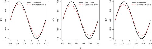
Figure 2. The true sine curve versus the estimated curve when n = 160 and $\tau =0.25$. Type I (left panel), Type II (middle panel), and Type III (right panel).

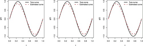
Table 1. Bias and MSE (in parenthesis) of the Bayesian estimates under ALD error distributions.

		n = 30			n = 80			n = 160
Type	Par	$\tau =0.25$	$\tau =0.5$	$\tau =0.75$	$\tau =0.25$	$\tau =0.5$	$\tau =0.75$	$\tau =0.25$	$\tau =0.5$	$\tau =0.75$
I	θ	$-$0.0120	$-$0.0052	0.0070	$-$0.0066	$-$0.0058	0.0047	$-$0.0027	0.0014	$-$0.0060
		(0.1009)	(0.0954)	(0.0997)	(0.0681)	(0.0554)	(0.0584)	(0.0406)	(0.0469)	(0.0388)
	${\text{β}}_1$	$-$0.0292	0.0389	$-$0.0033	0.0186	0.0005	0.0055	$-$0.0110	$-$0.0097	$-$0.0110
		(0.0670)	(0.0509)	(0.0671)	(0.0671)	(0.0196)	(0.0267)	(0.0126)	(0.0081)	(0.0155)
	${\text{β}}_2$	$-$0.0264	$-$0.0182	$-$0.0261	0.0157	$-$0.0177	0.0090	$-$0.0034	$-$0.0038	$-$0.0009
		(0.0926)	(0.0493)	(0.0850)	(0.0182)	(0.0182)	(0.0267)	(0.0122)	(0.0075)	(0.0146)
	${\text{β}}_3$	0.0442	0.0383	$-$0.0158	0.0139	0.0201	$-$0.0154	0.0139	0.0152	0.0177
		(0.0631)	(0.0479)	(0.0610)	(0.0269)	(0.0244)	(0.0324)	(0.0119)	(0.0092)	(0.0122)
	${\gamma }_1$	$-$0.0893	$-$0.0942	$-$0.0900	$-$0.0364	$-$0.0408	$-$0.1162	$-$0.0644	$-$0.0065	$-$0.0213
		(0.1575)	(0.1454)	(0.1915)	(0.1024)	(0.0749)	(0.1284)	(0.0559)	(0.0339)	(0.0499)
	${\gamma }_2$	0.0015	0.0313	0.0981	0.0207	0.0226	0.0358	0.0593	0.0254	0.0139
		(0.1468)	(0.1433)	(0.1753)	(0.0839)	(0.0688)	(0.1168)	(0.0772)	(0.0520)	(0.0589)
II	θ	$-$0.0087	$-$0.0030	0.0059	$-$0.0038	$-$0.0026	$-$0.0024	0.0026	$-$0.0049	$-$0.0065
		(0.0840)	(0.1052)	(0.0897)	(0.0611)	(0.0629)	(0.0546)	(0.0400)	(0.0425)	(0.0433)
	${\text{β}}_1$	0.0265	0.4839	0.0432	$-$0.0080	0.0228	$-$0.0007	$-$0.0113	0.0187	$-$0.0015
		(0.0635)	(0.0505)	(0.0570)	(0.0312)	(0.0201)	(0.0176)	(0.0129)	(0.0113)	(0.0123)
	${\text{β}}_2$	$-$0.0411	0.4839	0.0040	$-$0.0012	$-$0.0085	$-$0.0123	0.0159	$-$0.0079	$-$0.0195
		(0.0693)	(0.0693)	(0.0655)	(0.0287)	(0.0199)	(0.0282)	(0.0159)	(0.0080)	(0.0148)
	${\text{β}}_3$	0.0406	0.0220	0.0307	$-$0.0085	0.0036	0.0291	0.0025	0.0005	0.0188
		(0.0841)	(0.0507)	(0.0676)	(0.0206)	(0.0181)	(0.0293)	(0.0134)	(0.0089)	(0.0089)
	${\gamma }_1$	0.0621	0.0383	0.0893	0.0396	$-$0.0371	$-$0.0476	$-$0.0756	0.0191	$-$0.0602
		(0.1373)	(0.1458)	(0.1301)	(0.1004)	(0.1096)	(0.0876)	(0.0733)	(0.0438)	(0.0565)
	${\gamma }_2$	$-$0.0817	0.0101	$-$0.0500	0.0275	$-$0.0073	0.0253	0.0254	0.0124	0.0015
		(0.1657)	(0.1585)	(0.1790)	(0.1043)	(0.0946)	(0.1285)	(0.0546)	(0.0513)	(0.0646)
III	θ	0.0133	0.0054	0.0052	0.0066	$-$0.0017	0.0070	0.0082	$-$0.0029	0.0008
		(0.0902)	(0.0954)	(0.0875)	(0.0615)	(0.0555)	(0.0589)	(0.0385)	(0.0423)	(0.0438)
	${\text{β}}_1$	$-$0.0534	$-$0.0554	$-$0.1049	$-$0.0060	$-$0.0137	$-$0.0254	$-$0.0077	$-$0.0179	$-$0.0129
		(0.0661)	(0.0460)	(0.0911)	(0.0209)	(0.0224)	(0.0256)	(0.0131)	(0.0087)	(0.0107)
	${\text{β}}_2$	0.0289	0.0295	0.0555	0.0096	0.0385	0.0148	0.0118	0.0079	0.0185
		(0.0600)	(0.0457)	(0.0641)	(0.0295)	(0.0196)	(0.0175)	(0.0116)	(0.0103)	(0.0107)
	${\text{β}}_3$	$-$0.0658	$-$0.0488	$-$0.1025	$-$0.0290	$-$0.0215	$-$0.0144	$-$0.0238	$-$0.0240	$-$0.0113
		(0.0620)	(0.0662)	(0.0936)	(0.0342)	(0.0233)	(0.0251)	(0.0156)	(0.0112)	(0.0107)
	${\gamma }_1$	$-$0.3904	$-$0.3864	$-$0.4605	$-$0.2155	$-$0.1535	$-$0.1697	$-$0.0769	$-$0.0903	$-$0.1054
		(0.3888)	(0.3222)	(0.4177)	(0.1666)	(0.1105)	(0.1436)	(0.0640)	(0.0470)	(0.0619)
	${\gamma }_2$	0.2749	0.2181	0.2131	0.0822	0.0510	0.0975	0.0309	0.0627	0.0771
		(0.0619)	(0.2544)	(0.2342)	(0.1289)	(0.0997)	(0.1173)	(0.0548)	(0.0548)	(0.0651)

4.2. Quantile regression models with the non-ALD errors

To further illustrate the performance of the proposed Bayesian method, we consider the following three distributions for the errors

• Type A: ${ϵ}_{ij}\sim \mathrm{N}(\mu ,4)$, where μ is chosen such that the τth quantile is 0.

• Type B: ${ϵ}_{ij}\sim \mathrm{L}\mathrm{a}\mathrm{p}\mathrm{l}\mathrm{a}\mathrm{c}\mathrm{e}(\mu ,2)$, where μ is chosen such that the τth quantile is 0.

• Type C: ${ϵ}_{ij}\sim 0.3\mathrm{N}(\mu +1,1)+0.7\mathrm{N}(\mu ,4)$, where μ is chosen such that the τth quantile is 0.

Other simulation settings and the choices of the hyperparameters keep the same as the ones in Section 4.1. We consider n = 80 and $\tau =\{0.25,0.5,0.75\}$. We consider noninformative priors by setting ${\text{β}}_0=(0,0,0{)}^{\mathrm{T}}$ and ${\mathit{\gamma }}_0=(0,0{)}^{\mathrm{T}}$. Numerical results are provided in Table 2. It can be seen that under Type C, the MSEs of Bayesian estimates are smaller for all the parameters, especially for $\tau =\{0.25,0.75\}$ and that Bayesian estimates are quite accurate regardless of the errors under consideration.

Table 2. Bias and MSE (in parenthesis) of the Bayesian estimates under non-AL error distributions.

Distr.		n = 30			n = 80			n = 160
Type	Par	$\tau =0.25$	$\tau =0.5$	$\tau =0.75$	$\tau =0.25$	$\tau =0.5$	$\tau =0.75$	$\tau =0.25$	$\tau =0.5$	$\tau =0.75$
A	${\text{β}}_1$	$-$0.0207	$-$0.0271	$-$0.0327	$-$0.0361	$-$0.0098	$-$0.0328	$-$0.0115	0.0019	$-$0.0274
		(0.0388)	(0.0464)	(0.0469)	(0.0190)	(0.0154)	(0.0181)	(0.0092)	(0.0071)	(0.0109)
	${\text{β}}_2$	0.0314	0.0334	0.0319	0.0124	0.0136	0.0274	0.0012	0.0024	0.0105
		(0.0481)	(0.0333)	(0.0537)	(0.0139)	(0.0157)	(0.0176)	(0.0117)	(0.0083)	(0.0083)
	${\text{β}}_3$	$-$0.0390	$-$0.1331	$-$0.0460	$-$0.0201	$-$0.0200	$-$0.0246	$-$0.0074	$-$0.0181	$-$0.0111
		(0.0462)	(0.0549)	(0.0619)	(0.0184)	(0.0159)	(0.0142)	(0.0096)	(0.0084)	(0.0115)
	${\gamma }_1$	$-$0.3511	$-$0.3409	$-$0.3111	$-$0.1329	$-$0.1749	$-$0.1490	$-$0.1109	$-$0.0847	$-$0.0570
		(0.3303)	(0.3538)	(0.3077)	(0.1027)	(0.0985)	(0.0859)	(0.0496)	(0.0409)	(0.0528)
	${\gamma }_2$	0.1616	0.1717	0.1973	0.1402	0.0446	0.0677	0.0557	0.0144	$-$0.0239
		(0.2122)	(0.1398)	(0.2131)	(0.0819)	(0.0736)	(0.0672)	(0.0587)	(0.0386)	(0.0573)
B	${\text{β}}_1$	$-$0.0546	$-$0.0319	$-$0.0635	$-$0.0144	$-$0.0002	$-$0.0141	$-$0.0196	$-$0.0136	$-$0.0075
		(0.0792)	(0.0580)	(0.0706)	(0.0216)	(0.0208)	(0.0309)	(0.0153)	(0.0097)	(0.0125)
	${\text{β}}_2$	0.0478	0.0264	0.0322	0.0373	0.0178	$-$0.0082	0.0071	0.0136	0.0273
		(0.0874)	(0.0447)	(0.0715)	(0.0231)	(0.0154)	(0.0281)	(0.0154)	(0.0090)	(0.0135)
	${\text{β}}_3$	$-$0.0814	$-$0.0965	$-$0.1166	$-$0.0289	0.0005	$-$0.0160	$-$0.0097	$-$0.0058	$-$0.0091
		(0.0781)	(0.0876)	(0.1116)	(0.0206)	(0.0186)	(0.0259)	(0.0141)	(0.0125)	(0.0131)
	${\gamma }_1$	$-$0.4020	$-$0.3837	$-$0.4462	$-$0.1167	$-$0.1514	$-$0.1454	$-$0.1393	$-$0.0552	$-$0.0896
		(0.4017)	(0.3499)	(0.3815)	(0.1201)	(0.1158)	(0.1099)	(0.1122)	(0.0441)	(0.0789)
	${\gamma }_2$	0.2355	0.1080	0.1945	0.1040	0.1044	0.0913	0.0970	0.0391	0.0006
		(0.2878)	(0.1769)	(0.3284)	(0.1139)	(0.0915)	(0.1163)	(0.1020)	(0.0619)	(0.0716)
C	${\text{β}}_1$	$-$0.0438	$-$0.0344	$-$0.0562	$-$0.0066	$-$0.0194	$-$0.0144	$-$0.0165	$-$0.0110	$-$0.0108
		(0.0308)	(0.0253)	(0.0270)	(0.0080)	(0.0066)	(0.0081)	(0.0053)	(0.0053)	(0.0038)
	${\text{β}}_2$	0.0260	0.0415	0.0357	0.0226	0.0010	0.0100	0.0047	$-$0.0041	$-$0.0071
		(0.0223)	(0.0279)	(0.0312)	(0.0087)	(0.0083)	(0.0094)	(0.0055)	(0.0037)	(0.0047)
	${\text{β}}_3$	$-$0.0767	$-$0.0432	$-$0.0615	$-$0.0045	0.0040	$-$0.0126	$-$0.0019	$-$0.0031	$-$0.0152
		(0.0309)	(0.0233)	(0.0245)	(0.0072)	(0.0064)	(0.0092)	(0.0066)	(0.0046)	(0.0054)
	${\gamma }_1$	$-$0.1808	$-$0.2185	$-$0.1716	$-$0.0950	$-$0.0337	$-$0.1084	$-$0.0825	$-$0.0366	$-$0.0885
		(0.1779)	(0.1750)	(0.2245)	(0.0603)	(0.0497)	(0.0641)	(0.0344)	(0.0285)	(0.0383)
	${\gamma }_2$	0.0914	0.0746	0.0587	0.0182	0.0400	0.0670	0.0260	0.0380	0.0475
		(0.1283)	(0.1305)	(0.1276)	(0.0420)	(0.0402)	(0.0534)	(0.0295)	(0.0326)	(0.0333)

5. Real data application: the multiCenter AIDS cohort study

In this section, we consider the MultiCenter AIDS Cohort Study (MACS) data, which is available in the ‘timereg’ package (Scheike & Zhang, 2011). The MACS data set consists of 283 human immunodeficiency virus (HIV) status of homosexual men. This data set has been widely used to study the mean CD4 percentage depletion over time and the effects of other physical status, including age of the patient at the start of the trial, smoking status, and the post-infection CD4 percentage; see, for example, Fan and Li (2004); Xu et al. (2016); Zhao and Xue (2010). Owing to the difference of the trend of CD4 depletion between high CD4 percentage and low CD4 percentage patients, this data set is of specific interest to us for the implementation of the proposed Bayesian quantile SPMED models.

Let $y_{ij}$ be the observation of CD4 percentage at the current visit, $x_{ij1}$ be the smoking status (0 for non-smoker and 1 for smoker), $x_{ij2}$ be the age of the patient at the start of the trial, and $x_{ij3}$ be the post-infection CD4 percentage. To avoid the need of an intercept, it is assume that the response $\mathbf{y}$ is zero centered. We also assume that the variance of the random effect $v_i$ has a linear relationship with two predictors $z_{i1}=\frac{1}{m_i}\sum _{j=1}^{m_i}{x}_{ij1}$ and $z_{i2}=\frac{1}{m_i}\sum _{j=1}^{m_i}{x}_{ij3}$. The Bayesian quantile SPMED regression model can be written as $y_{ij}={\mathbf{x}}_{ij}^{\mathrm{T}}\text{β}+g\left(t_{ij}\right)+v_i+k_1{e}_{ij}+r_{ij}\sqrt{k_2\theta e_{ij}},$ where ${\mathbf{x}}_{ij}=(x_{ij1},x_{ij2},x_{ij3}{)}^{\mathrm{T}}$, $\text{β}=({\text{β}}_1,{\text{β}}_2,{\text{β}}_3{)}^{\mathrm{T}}$, $k_1=\frac{1-2\tau }{\tau (1-\tau )}$, and $k_2=\frac{2}{\tau (1-\tau )}$. Here, $e_{ij}\sim \mathcal{E}\left({\theta }^{-1}\right)$, $r_{ij}\sim \mathrm{N}(0,1)$, and $v_i\sim \mathrm{N}(0,{\sigma }_i^2)$ with ${\sigma }_i^2={\gamma }_1{z}_{i1}+{\gamma }_2{z}_{i2}$ for $i=1,2,\dots ,283,j=1,2,\dots ,m_i$.

We are interested in investigating the relationship between the mean CD4 percentage $g\left(t_{ij}\right)$ and time $t_{ij}$ at different quantile levels $\tau =\{0.05,0.25,0.5,0.75,0.95\}$. Due to a lack of prior knowledge, we set all the hyperparameters to be small and let initial values of all the unknown parameters be 0. For the implementation of the Metropolis-Hastings algorithm for sampling $\mathit{\gamma }$, we set ${\sigma }_{\gamma }^2=4$ to achieve approximate acceptance rates of about 35% (Gelman & Gilks, 1996). For each quantile level, we run the proposed MCMC-based sampling algorithm 55,000 iterations, discard the first 5,000 as the burn-in period, and then perform a thinning factor of 10, leading to a total number of 5,000 samples for conducting the posterior inference.

Figures 3 and 4 depict the trace and density plots of 5,000 posterior samples of the model parameters. It can be seen from these figures that the MCMC chains of all the parameters rapidly converge to their stationary distributions. Furthermore, we present the autocorrelation function (ACF) plot to in Figure 5 check the autocorrelations between the posterior samples of all the parameters, which shows that the autocorrelations between posterior samples decline to zero at a very fast rate. Similar results are also observed with respect to other quantiles and are not shown here for simplicity. We also conduct the run length control diagnostic of Raftery and Lewis (1992) and the convergence diagnostic test statistic of Geweke (1992) at a significance level of 5$\mathrm{\%}$, which reconfirm that there is no evidence of lack of convergence of all the MCMC chains.

Figure 3. The trace plot and density plot of 5,000 posterior samples of ($\theta ,{\gamma }_1,{\gamma }_2$) when $\tau =0.5$.

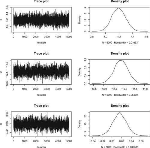
Figure 4. The trace plot and density plot of 5,000 posterior samples of (${\text{β}}_1,{\text{β}}_2,{\text{β}}_3$) when $\tau =0.5$.

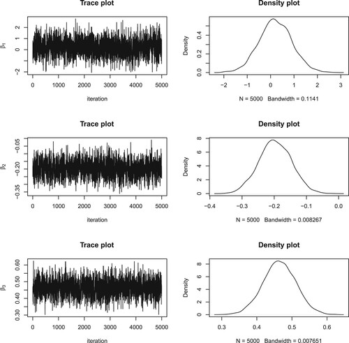
Figure 5. The ACF plot of 5,000 posterior samples of the unknown parameters when $\tau =0.5$.

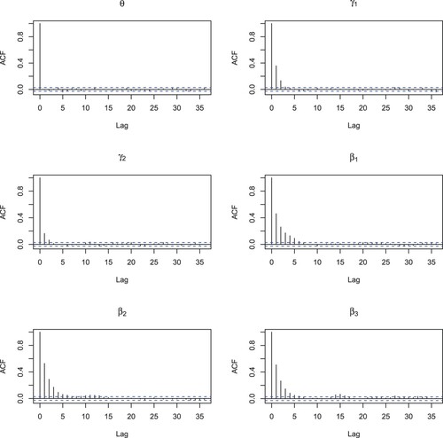
Table 3 summarizes Bayesian estimates (EST) of the unknown parameters $(\theta ,{\varphi }^2,\text{β},\mathit{\gamma })$ and their standard deviation estimates (SD). Figure 6 depicts the estimated CD4 depletion trends under five different quantile levels. As one expects, the CD4 depletion trends are quite distinct among diverse groups of patients. For instance, for the patients who have a high CD4 level around 50, their CD4 percentages almost get back to their original level after 6 years. Other patients' CD4 percentages could decrease quickly after an infection, whereas they would increase at the end. This observation indicates drug usage can be distributed according to the patients' starting CD4 percentages. It deserves mentioning that our results at $\tau =0.5$ are in good agreement with the ones by fitting the local linear fitting method of Fan and Li (2004) and by using the semiparametric varying-coefficient partially linear models of Zhao and Xue(2011).

Figure 6. The mean CD4 percentage $g\left(t_{ij}\right)$ vs time $t_{ij}$ at the 5 different quantile levels.

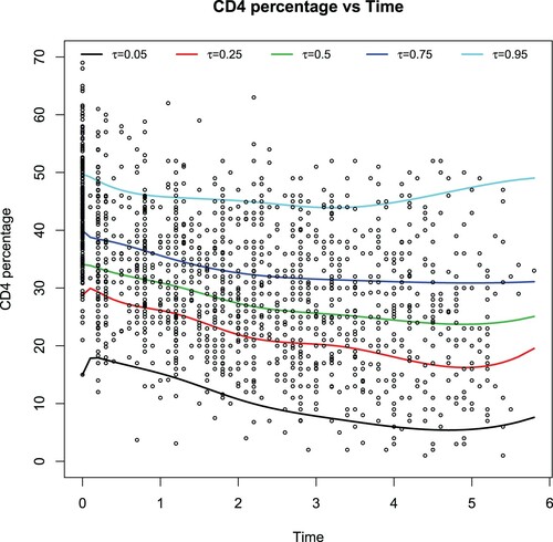
Table 3. The Bayesian estimates of the unknown parameters in the MACS data.

	$\tau =0.05$		$\tau =0.25$		$\tau =0.50$		$\tau =0.75$		$\tau =0.95$
Parameter	EST	SD	EST	SD	EST	SD	EST	SD	EST	SD
θ	13.2042	0.4753	4.4680	0.1191	4.1952	0.0996	4.5017	0.1186	13.2282	0.4892
${\text{β}}_1$	2.0707	1.6743	−0.7671	0.6996	0.2107	0.7003	1.5214	0.6853	−0.7996	1.7156
${\text{β}}_2$	0.0381	0.1144	−0.1395	0.0469	−0.1970	0.0505	−0.1148	0.0434	0.0131	0.1080
${\text{β}}_3$	0.1565	0.1067	0.4235	0.0458	0.4644	0.0467	0.4884	0.0390	0.4195	0.0984
${\gamma }_1$	−0.0441	0.9475	−11.8450	0.3887	−12.1508	0.3350	−11.3275	0.3900	−0.2008	0.9355
${\gamma }_2$	0.0068	0.1041	0.0267	0.0168	0.0160	0.0141	0.0081	0.0159	−0.0525	0.0997

6. Concluding remarks

In this paper, we developed Bayesian methods for parameter estimation in quantile semiparametric mixed-effects double regression models by modeling the variance of the mixed-effects as a function of predictors. A Bayesian hierarchical model was developed and an efficient MCMC-based sampling algorithm was proposed for performing the full posterior inference. Numerical results from both simulation studies and a real data application showed that the proposed procedures perform well in general settings and can accurately estimate the parameters of interest under different scenarios. It is known that variable selection is as important as parameter estimation in modeling the longitudinal data, and for future work, we conduct Bayesian variable selection in quantile semiparametric mixed-effects double regression models.

Acknowledgements

The authors greatly appreciate the two reviewers for their thoughtful comments and suggestions, which have improved the quality of the manuscript. This work was based on the first author's dissertation research which was supervised by the corresponding author. Dr. Wu was supported by the National Natural Science Foundation of China under grant 11861041. Drs. Keying Ye and Min Wang were partially supported by a grant from the UTSA Vice President for Research, Economic Development, and Knowledge Enterprise at the University of Texas at San Antonio.

Disclosure statement

No potential conflict of interest was reported by the author(s).

Additional information

Notes on contributors

Duo Zhang

Duo Zhang is a statistician and his research interests include quantile regression, statistical analysis, and applications.

Liucang Wu

Liucang Wu is a professor of Statistics in the Faculty of Science at Kunming University of Science and Technology. His research interests include Bayesian analysis, statistical decision theory, multivariate analysis, and statistical applications.

Keying Ye

Keying Ye is a professor of Statistics in the Department of Management Science and Statistics at the University of Texas at San Antonio. His research interests include Bayesian analysis, statistical inference and decision theory, and statistical applications.

Min Wang

Min Wang is an associate professor of Statistics in the Department of Management Science and Statistics at the University of Texas at San Antonio. His research interests include Bayesian statistics, high dimensional inference, statistical applications, and machine learning.

Appendix

The Metropolis–Hastings algorithm for sampling $\mathit{\gamma }$ in Algorithm 1 is summarized as follows. We choose the commonly used multivariate normal distribution as the proposal distribution (Chib & Greenberg, 1994), denoted by ${\mathrm{N}}_q({\mathbf{m}}^{\left(k\right)},{\sigma }_{\gamma }^2{V}^{\left(k\right)})$ with $\begin{array}{rl}{\mathbf{m}}^{\left(k\right)}& =\arg max\log p(\mathit{\gamma }|{\mathbf{v}}^{\left(k\right)},\mathbf{y},\mathbf{X},\mathbf{Z},\mathbf{t}),\\ V^{\left(k\right)}& =\left\{\right(-H{)}^{-1}{\}}_{\mathit{\gamma }=\mathbf{m}},H=\frac{{\mathrm{\partial }}^{2}p(\mathit{\gamma }|{\mathbf{v}}^{\left(k\right)},\mathbf{y},\mathbf{X},\mathbf{Z},\mathbf{t})}{\mathrm{\partial }\mathit{\gamma }\mathrm{\partial }{\mathit{\gamma }}^{\mathrm{T}}},\end{array}$ where $H$ is the Hessian matrix and ${\sigma }_{\gamma }^2$ is chosen such that the average acceptance rate is between 0.25 and 0.45 (Gelman & Gilks, 1996). For the $(k+1)$th iteration, we sample ${\mathit{\gamma }}^{\left(k\right)}$ by the following two steps:

1. Generate a new candidate ${\mathit{\gamma }}^{\star }$ from the proposal distribution ${\mathrm{N}}_q({\mathbf{m}}^{\left(k\right)},{\sigma }_{\gamma }^2{V}^{\left(k\right)})$.

2. Let ${\mathit{\gamma }}^{\left(k\right)}=\left\{\begin{array}{ll}{\mathit{\gamma }}^{\star },& \text{if Unif }(0,1)\le \omega ({\mathit{\gamma }}^{\star },{\mathit{\gamma }}^{\left(k\right)}),\\ {\mathit{\gamma }}^{\left(k\right)},& \text{otherwise},\end{array}\right.,$ where $\omega ({\mathit{\gamma }}^{\star },{\mathit{\gamma }}^{\left(k\right)})$ is the acceptance ratio given by $\omega ({\mathit{\gamma }}^{\star },{\mathit{\gamma }}^{\left(k\right)})=min\left\{1,\frac{p({\mathit{\gamma }}^{\star }|{\mathbf{v}}^{\left(k\right)},\mathbf{y},\mathbf{X},\mathbf{Z},\mathbf{t})}{p({\mathit{\gamma }}^{\left(k\right)}|{\mathbf{v}}^{\left(k\right)},\mathbf{y},\mathbf{X},\mathbf{Z},\mathbf{t})}\right\}.$

References

- Aitkin, M. (1987). Modelling variance heterogeneity in normal regression using GLIM. Applied Statistics, 36(2), 332–339. https://doi.org/https://doi.org/10.2307/2347792
- Alhamzawi, R., & Ali, H. (2018). Bayesian quantile regression for ordinal longitudinal data. Journal of Applied Statistics, 45, 815–828. https://doi.org/https://doi.org/10.1080/02664763.2017.1315059
- Cepeda, E., & Gamerman, D. (2000). Bayesian modeling of variance heterogeneity in normal regression models. Brazilian Journal of Probability and Statistics, 14, 207–221. https://doi.org/https://doi.org/10.2307/43600978
- Chen, X., & Tang, N. (2010). Bayesian analysis of semiparametric reproductive dispersion mixed-effects models. Computational Statistics & Data Analysis, 54, 2145–2158. https://doi.org/https://doi.org/10.1016/j.csda.2010.03.022
- Chen, Y., & Ye, K. (2009). Bayesian hierarchical modelling on dual response surfaces in partially replicated designs. Quality Technology & Quantitative Management, 6, 371–389. https://doi.org/https://doi.org/10.1080/16843703.2009.11673205
- Chen, Y., & Ye, K. (2011). A Bayesian hierarchical approach to dual response surface modelling. Journal of Applied Statistics, 38, 1963–1975. https://doi.org/https://doi.org/10.1080/02664763.2010.545106
- Chib, S., & Greenberg, E. (1994). Bayes inference in regression models with ARMA (p,q) errors. Journal of Econometrics, 64, 183–206. https://doi.org/https://doi.org/10.1016/0304-4076(94)90063-9
- Fan, J., & Gijbels, I. (1996). Local polynomial modelling and its applications. In Monographs on statistics and applied probability, vol. 66. Chapman & Hall.
- Fan, J., & Li, R. (2004). New estimation and model selection procedures for semiparametric modeling in longitudinal data analysis. Journal of the American Statistical Association, 99, 710–723. https://doi.org/https://doi.org/10.1198/016214504000001060
- Fonseca, T., Ferreira, Marco A., & Migon, H. (2008). Objective Bayesian analysis for the student-t regression model. Biometrika, 95, 325–333. https://doi.org/https://doi.org/10.1093/biomet/asn001
- Gelman, A. R., & Gilks, W. (1996). Efficient metropolis jumping rules. In Bayesian statistics, 5 (Alicante, 1994), (pp. 599–607). Oxford Sci. Publ. Oxford University Press.
- Geraci, M. (2019). Additive quantile regression for clustered data with an application to children's physical activity. Journal of the Royal Statistical Society. Series C, Applied Statistics, 68, 1071–1089. https://doi.org/https://doi.org/10.1111/rssc.2019.68.issue-4
- Geraci, M., & Bottai, M. (2014). Linear quantile mixed models. Statistics and Computing, 24, 461–479. https://doi.org/https://doi.org/10.1007/s11222-013-9381-9
- Geweke, J. (1992). Evaluating the accuracy of sampling-based approaches to the calculation of posterior moments. In Bayesian statistics, 4 (Peñíscola, 1991) (pp. 169–193). Oxford University Press.
- He, X., Fung, W. K., & Zhu, Z. (2005). Robust estimation in generalized partial linear models for clustered data. Journal of the American Statistical Association, 100, 1176–1184. https://doi.org/https://doi.org/10.1198/016214505000000277
- Hunter, D., & Lange, K. (2000). Quantile regression via an MM algorithm. Journal of Computational and Graphical Statistics, 9, 60–77. https://doi.org/https://doi.org/10.2307/1390613
- Kai, B., Li, R., & Zou, H. (2011). New efficient estimation and variable selection methods for semiparametric varying-coefficient partially linear models. The Annals of Statistics, 39, 305–332. https://doi.org/https://doi.org/10.1214/10-AOS842
- Kang, S., Liu, G., Qi, H., & Wang, M. (2018). Bayesian variance changepoint detection in linear models with symmetric heavy-tailed errors. Computational Economics, 52, 459–477. https://doi.org/https://doi.org/10.1007/s10614-017-9690-8
- Koenker, R., & Bassett, Jr. G. (1978). Regression quantiles. Econometrica, 46, 33–50. https://doi.org/https://doi.org/10.2307/1913643
- Koenker, R., Chernozhukov, V., He, X., & Peng, L. (2018). Handbook of quantile regression. In Chapman & Hall/CRC handbooks of modern statistical methods. CRC Press.
- Koenker, R., & Park, B. (1996). An interior point algorithm for nonlinear quantile regression. Journal of Econometrics, 71, 265–283. https://doi.org/https://doi.org/10.1016/0304-4076(96)84507-6
- Kotz, S., Kozubowski, T. J., & Podgórski, K. (2001). The laplace distribution and generalizations: A revisit with applications to communications, economics, engineering, and finance. Birkhäuser Boston, Inc.
- Kozumi, H., & Kobayashi, G. (2011). Gibbs sampling methods for Bayesian quantile regression. Journal of Statistical Computation and Simulation, 81, 1565–1578. https://doi.org/https://doi.org/10.1080/00949655.2010.496117
- Lombardia, M. J., & Sperlich, S. (2007). Semiparametric inference in generalized mixed effects models. Journal of the Royal Statistical Society. Series B. Statistical Methodology, 70, 913–930. https://doi.org/https://doi.org/10.1111/j.1467-9868.2008.00655.x
- Raftery, A., & Lewis, S. (1992). [Practical Markov Chain Monte Carlo]: comment: one long run with diagnostics: implementation strategies for Markov Chain Monte Carlo. Statistical Science, 7, 493–497. https://doi.org/https://doi.org/10.1214/ss/1177011143
- Scheike, T. H., & Zhang, M. -J. (2011). Analyzing competing risk data using the R timereg package. Journal of Statistical Software, 38, 1–15. https://doi.org/https://doi.org/10.18637/jss.v038.i02
- Tang, N., & Duan, X. (2012). A semiparametric Bayesian approach to generalized partial linear mixed models for longitudinal data. Computational Statistics & Data Analysis, 56, 4348–4365. https://doi.org/https://doi.org/10.1016/j.csda.2012.03.018
- Tian, Y., Li, E., & Tian, M. (2016). Bayesian joint quantile regression for mixed effects models with censoring and errors in covariates. Computational Statistics, 31, 1031–1057. https://doi.org/https://doi.org/10.1007/s00180-016-0659-1
- Tian, Y., & Song, X. (2020). Bayesian bridge-randomized penalized quantile regression. Computational Statistics & Data Analysis, 144, 106876, 16. https://doi.org/https://doi.org/10.1016/j.csda.2019.106876
- Tian, Y., Tian, M., & Zhu, Q. (2014). Linear quantile regression based on EM algorithm. Communication in Statistics – Theory and Methods, 43, 3464–3484. https://doi.org/https://doi.org/10.1080/03610926.2013.766339
- Waldmann, E., Kneib, T., Yue, Y. R., Lang, S., & Flexeder, C. (2013). Bayesian semiparametric additive quantile regression. Statistical Modelling, 13, 223–252. https://doi.org/https://doi.org/10.1177/1471082X13480650
- Wu, L., Tian, G.-L., Zhang, Y.-Q., & Ma, T. (2017). Variable selection in joint location, scale and skewness models with a skew-t-normal distribution. Statistics and Its Interface, 10, 217–227. https://doi.org/https://doi.org/10.4310/SII.2017.v10.n2.a6
- Xu, D., Zhang, Z., & Wu, L. (2016). Bayesian analysis for semiparametric mixed-effects double regression models. Hacettepe Journal of Mathematics and Statistics, 41, 279–296.
- Yang, Y., Wang, H. J., & He, X. (2016). Posterior inference in Bayesian quantile regression with asymmetric Laplace likelihood. International Statistical Review, 84, 327–344. https://doi.org/https://doi.org/10.1111/insr.12114
- Yu, K., & Moyeed, R. A. (2001). Bayesian quantile regression. Statistics & Probability Letters, 54, 437–447. https://doi.org/https://doi.org/10.1016/S0167-7152(01)00124-9
- Zhang, H., Huang, Y., Wang, W., Chen, H., & Langland-Orban, B. (2019). Bayesian quantile regression-based partially linear mixed-effects joint models for longitudinal data with multiple features. Statistical Methods in Medical Research, 28, 569–588. https://doi.org/https://doi.org/10.1177/0962280217730852
- Zhao, P., & Xue, L. (2010). Variable selection for semiparametric varying coefficient partially linear errors-in-variables models. Journal of Multivariate Analysis, 101, 1872–1883. https://doi.org/https://doi.org/10.1016/j.jmva.2010.03.005
- Zhao, P., & Xue, L. (2011). Variable selection for semiparametric varying-coefficient partially linear models with missing response at random. Acta Mathematica Sinica, English Series, 27, 2205–2216. https://doi.org/https://doi.org/10.1007/s10114-011-9200-1