Robust sequential design for piecewise-stationary multi-armed bandit problem in the presence of outliers

ABSTRACT

The multi-armed bandit (MAB) problem studies the sequential decision making in the presence of uncertainty and partial feedback on rewards. Its name comes from imagining a gambler at a row of slot machines who needs to decide the best strategy on the number of times as well as the orders to play each machine. It is a classic reinforcement learning problem which is fundamental to many online learning problems. In many practical applications of the MAB, the reward distributions may change at unknown time steps and the outliers (extreme rewards) often exist. Current sequential design strategies may struggle in such cases, as they tend to infer additional change points to fit the outliers. In this paper, we propose a robust change-detection upper confidence bound (RCD-UCB) algorithm which can distinguish the real change points from the outliers in piecewise-stationary MAB settings. We show that the proposed RCD-UCB algorithm can achieve a nearly optimal regret bound on the order of $O\left(\sqrt{SKT\log T}\right)$, where T is the number of time steps, K is the number of arms and S is the number of stationary segments. We demonstrate its superior performance compared to some state-of-the-art algorithms in both simulation experiments and real data analysis. (See https://github.com/woaishufenke/MAB_STRF.git for the codes used in this paper.)

Keywords:

• Change-point detection
• noisy data
• online learning
• truncated loss

1. Introduction

The multi-armed bandit (MAB) problem, originally introduced by Thompson (1933), studies how a decision-maker adaptively selects one from a series of alternative arms based on the historical observations of each arm and receives a reward accordingly (Lai & Robbins, 1985). The MAB is a fundamental problem to many online learning applications, such as the online recommendation system (Li et al., 2016), the dynamic spectrum access in communication system (Alaya-Feki et al., 2008) and the computational advertisement (Buccapatnam et al., 2017). A common goal of the sequential designs, i.e. the bandit algorithms, is to minimise the regret of the decision maker, where the regret refers to the expectation of the difference between the total rewards collected by playing the arm with the highest expected rewards and the total rewards obtained by the algorithms (Auer, 2002). To achieve this goal, decision-makers need to make a trade-off between exploring the environment to find the most profitable arms and exploiting the current empirically best arms as often as possible.

There is a rich literature studying classic MAB problems (Lattimore & Szepesvári, 2020), including the stochastic bandit models (Lai & Robbins, 1985) and the adversarial bandit models (Auer, Cesa-Bianchi, Freund et al., 2002). The former assumes that the reward distributions of all arms are time-invariant, and the latter assumes that the reward distributions of all arms change adversarially at all time steps. Yet, neither of these two assumptions may be realistic in many real-world applications, where the reward distributions do vary with time but much less frequently compared to what the adversarial bandit model assumes (Alaya-Feki et al., 2008); Yu & Mannor, 2009). In this paper, we focus on such piecewise-stationary MAB problems where the reward distributions are piecewise-constant and may shift at some unknown time steps called the change points; that is, we focus on MAB problems with mean changes.

In the current literature, two major approaches are proposed for the piecewise-stationary bandit problems: the passively adaptive policies and the actively adaptive policies (Liu et al., 2018). The passively adaptive policies adapt to the changes via adjusting the weights on the rewards. Specifically, the discounted upper confidence bound (D-UCB) algorithm discounts the weights on the old rewards and thus allocates larger weights on the recent ones when computing the UCB index of each arm (Kocsis & Szepesvári, 2006). The D-UCB algorithm achieves a regret bound on the order of $O(K\sqrt{ST}\log T)$, where T is the number of time steps, K is the number of arms and S is the number of stationary segments (Garivier & Moulines, 2011). Based on the D-UCB, the Sliding-Window UCB (SW-UCB) algorithm chooses only the most recent τ rewards in computing the UCB index, which achieves a regret $O\left(K\sqrt{ST\log T}\right)$ (Garivier & Moulines, 2011). Other passively adaptive policies include the EXP3.S (Auer, Cesa-Bianchi, Freund et al., 2002), the SHIFTBAND (Auer, 2002) and the Rexp3 (Besbes et al., 2014) algorithms.

The actively adaptive policies monitor the reward distributions by a change-detection (CD) algorithm. Their bandit algorithms will be reset once a change point is detected. The actively adaptive policies often have better performance compared to the passively adaptive policies in practice (Cao et al., 2019). For detecting the change points, the CUSUM-UCB algorithm (Liu et al., 2018) adopts the CUSUM method, and the Adapt-EvE algorithm (Hartland et al., 2007) and the adaptive SW-UCL algorithm (Srivastava et al., 2014) employ the Page-Hinkley Test (Hinkley, 1971). Some other available actively adaptive policies include the Bayesian CD algorithm (Mellor & Shapiro, 2013), the windowed mean-shift detection algorithm (Yu & Mannor, 2009) and the EXP3.R algorithm (Allesiardo & Féraud, 2015). To our best knowledge, the Monitored-UCB (M-UCB) algorithm by Cao et al. (2019) is the currently most efficient method. The M-UCB achieves a nearly optimal regret bound on the order of $O\left(\sqrt{SKT\log T}\right)$ without strong parametric assumptions, and performs very well in practical applications. In this paper, we use the M-UCB as the benchmark method.

Unexpected data changes may significantly affect the data quality, which can invalidate the classic MAB algorithms (Cao et al., 2019). Such data offsets may come from the trend changes or the outliers. Here an outlier means a data point with an unusually large or small value. In the current literature, most methods on non-stationary MAB problems only consider the former but ignore the latter (Allesiardo & Féraud, 2015). In many state-of-the-art algorithms on piecewise-stationary MAB problems (Cao et al., 2019; Kaufmann et al., 2012; Liu et al., 2018), once their CD algorithms identify a change point, the embedded bandit algorithms will reset the current optimal arms and try to learn new ones. Since they often cannot distinguish the real trend changes from large outliers, their CD algorithms tend to infer additional change points to fit the outliers. When there are many scattered outliers, the reset strategy adopted in these algorithms will greatly reduce their efficiency and increase the computational complexity. Specifically, the M-UCB algorithm (Cao et al., 2019) relies on comparing the statistical distances between data segments and the thresholds to test the significance of the trend offsets in the local data, which can be very sensitive to the outliers.

In this paper, we propose a robust change-detection upper confidence bound (RCD-UCB) algorithm which can distinguish the real change points from the outliers for non-stationary MAB problems. The proposed RCD-UCB algorithm includes a new trend offset detection using truncated loss functions to eliminate the impacts of outliers. We show that the RCD-UCB algorithm can achieve a nearly optimal regret bound on the order of $O\left(\sqrt{SKT\log T}\right)$ for piecewise-stationary MAB problems, which is of the same order as the bound in Cao et al. (2019). We demonstrate the superior performance of the RCD-UCB via three simulation studies and a real data analysis on metalwork factory machining, where the proposed algorithm can significantly reduce the cumulative regrets compared to some currently popular methods.

The remainder of this paper is organised as follows. In Section 2, we first formulate the piecewise-stationary MAB problems, then introduce the proposed RCD-UCB algorithm, and finally discuss its theoretical regret bound. In Section 3, we demonstrate the superior performance of the RCD-UCB via three simulation studies and a real data example. Section 4 concludes this work and discusses some future works. A brief description of the classic UCB1 algorithm (Auer, Cesa-Bianchi, Freund et al., 2002) and all proofs are relegated to the Appendix.

2. The RCD-UCB algorithm for piecewise-stationary MAB problems in the presence of outliers

2.1. Problem formulation

In an MAB problem, denote $\mathcal{K}=\{1,\dots ,K\}$ as the set of swing arms and $\mathcal{T}=\{1,\dots ,T\}$ as the set of time slots. At each time slot $t\in \mathcal{T}$, the learning agent chooses an arm $A_t\in \mathcal{K}$ and gets a reward $X_{A_t,t}\in [0,1]$ which can be generalised to any bounded interval. The reward sequence $\{X_{k,t}{\}}_{t=1,\dots ,T}$ for the arm $k\in \mathcal{K}$ can be seen as a series of independent random variables from potentially different distributions. Let $E\left(X_{k,t}\right)$ be the expectation of reward $X_{k,t}$ at the time slot t. Let $k_t^{\ast }$ be the selector having the maximum expected reward at time t, i.e. $E\left(X_{k_t^{\ast },t}\right)=\underset{k\in \mathcal{K}}{max}E\left(X_{k,t}\right)$, $t\in \mathcal{T}$. The learning agent wants to make a series of right decisions about the playing arms $\{A_t,t\in \mathcal{T}\}$ to maximise the expected cumulative reward, i.e. $maxE\left(\sum _{t=1}^T{X}_{A_t,t}\right)$, for the entire T time periods (Srivastava et al., 2014). Equivalently, it is to minimise the T-step cumulative regret (Cao et al., 2019): (1) $\mathcal{R}\left(T\right)=\sum _{t=1}^T\underset{k\in \mathcal{K}}{max}E\left(X_{k,t}\right)-E\left(\sum _{t=1}^T{X}_{A_t,t}\right),$(1) i.e., the expected total loss of playing arms $\{A_t,t\in \mathcal{T}\}$.

For the piecewise-stationary MAB scenario, define $F_t\left(k\right)$ as the reward distribution of the kth selected arm at time t. The reward $X_{k,t}$ is independently sampled from $F_t\left(k\right)$, both across arms and across time slots. Here, the $F_t\left(k\right)$ can have various types, such as uniform, Bernoulli and exponential distributions. When outliers exist, unusually small or large rewards are encountered, which may come from the reward distributions with extreme probabilities or simply from collection errors.

Let S be the number of piecewise-stationary segments in the reward sequence: $\begin{array}{rl}S& =1+\sum _{t=1}^{T-1}\\ & \times \mathbb{I}\left\{E\right(X_{k,t})\ne E(X_{k+1,t})\text{for at least one}k\in \mathcal{K}\},\end{array}$where $\mathbb{I}\{\cdot \}$ represents the indicator function. Here, we have S−1 change points represented by $p_1,p_2,\dots ,p_{S-1}$, which are defined to be the time slots that the changes occur. For notation consistency, we set $p_0=0$ and $p_S=T$. Within the same segments, the rewards follow the same distributions, but among different segments, the reward distributions can be different. Similar to Liu et al. (2018) and Cao et al. (2019), we consider using the means to describe the trends in the non-stationary data. Let ${\mu }_k^{\left(j\right)}=E\left(X_{k,p_{j-1}+1}\right)=\cdots =E\left(X_{k,p_j}\right)$ be the mean response for the kth arm in the jth data segment where $k\in \mathcal{K}$ and $j=1,\dots ,S$. We consider the cases where there exists at least one arm $k\in \mathcal{K}$ such that ${\mu }_k^{\left(j\right)}\ne {\mu }_k^{(j+1)}$ ($j=1,\dots ,S-1$) and $|{\mu }_k^{\left(j\right)}-{\mu }_k^{(j+1)}|$ is not very small (see Assumption 2.1(b)) for detectability, which excludes infinitesimal mean shift and is a reasonable assumption in practice (Liu et al., 2018). There is no requirement on the shape of the reward distribution. Note that, if we set S = 1 in our framework, it becomes the classic stochastic bandit model (Besbes et al., 2014); if we set $S=T$, it becomes the classic adversarial bandit model (Garivier & Moulines, 2011).

2.2. The RCD-UCB algorithm

In this part, we propose a novel algorithm framework for piecewise-stationary MAB problems in the presence of outliers. It improves the current change-detection UCB framework by incorporating a data-driven tail truncation strategy that can distinguish the real change points from the outliers. Current popular tail truncation methods to restrict unexpected changes caused by extreme values include:

(1) Huber loss: $L({\mu }_j,{\mu }_{j^{\prime }})=\left\{\begin{array}{ll}({\mu }_j-{\mu }_{j^{\prime }}{)}^2& \mathrm{i}\mathrm{f}|{\mu }_j-{\mu }_{j^{\prime }}|<a\\ 2a|{\mu }_j-{\mu }_{j^{\prime }}|-a^2& \mathrm{o}\mathrm{t}\mathrm{h}\mathrm{e}\mathrm{r}\mathrm{w}\mathrm{i}\mathrm{s}\mathrm{e},\end{array}\right.$(2) the biweight loss: $L({\mu }_j,{\mu }_{j^{\prime }})=\left\{\begin{array}{ll}({\mu }_j-{\mu }_{j^{\prime }}{)}^2& \mathrm{i}\mathrm{f}|{\mu }_j-{\mu }_{j^{\prime }}|<a\\ a^2& \mathrm{o}\mathrm{t}\mathrm{h}\mathrm{e}\mathrm{r}\mathrm{w}\mathrm{i}\mathrm{s}\mathrm{e},\end{array}\right.$and (3) if interest lies in changes in the uth quantile for 0<u<1: $L({\mu }_j,{\mu }_{j^{\prime }})=\left\{\begin{array}{ll}2u({\mu }_j-{\mu }_{j^{\prime }})& \mathrm{i}\mathrm{f}{\mu }_j>{\mu }_{j^{\prime }}\\ 2(1-u)({\mu }_{j^{\prime }}-{\mu }_j)& \mathrm{o}\mathrm{t}\mathrm{h}\mathrm{e}\mathrm{r}\mathrm{w}\mathrm{i}\mathrm{s}\mathrm{e}.\end{array}\right.$In particular, if u = 0.5, the loss function (3) reduces to $|{\mu }_j-{\mu }_{j^{\prime }}|.$ The proposed algorithm framework can incorporate various tail truncation methods. Yet, we do not recommend to use the loss function (3) since the mean changes are of interest here. Compared to the Huber loss, our proposed algorithm with the biweight loss generally have better performance by some simulation explorations. Thus, in this paper, we focus on using the biweight loss in the change point detection, where the parameter a is determined via a data-driven approach.

In Algorithm 1, we show our robust change detection (RCD) method using the biweight loss. It considers a change point detection strategy based on comparing running sample means over a sliding window. Here, the window width w and the statistical distance threshold b are tuning parameters, which can be chosen empirically or based on the theoretical results in Section 2.3. The selected w must be even since the means of the first and second halves of the running samples ($Y_1,\dots ,Y_w$) are compared. The biweight loss function bounds the absolute differences of sample means at most a, where parameter a is updated through historical data and controlled by the tuning parameter α in Algorithm 2. This simple RCD algorithm has minimum parameter specification and thus is computationally efficient.

Next, we show the proposed RCD-UCB algorithm in Algorithm 2 whose parameters mainly include the total number of time slots T, the number of arms K, the policy rotation parameter γ, the delay parameter D and the outlier truncation probability α. The tuning parameter γ controls the fraction of the uniform sampling used for feeding the RCD algorithm (line 4), which can be determined based on the theoretical results in Section 2.3. For the kth arm, let $a_k$ denote the upper bound for calculating the truncation distance in the biweight loss function (line 3 in Algorithm 1) and ${\mathcal{L}}_k$ be the list used to record the offset distances (line 15) when each detection is not significant. The tuning parameter $\alpha \in (0,1)$ controls the values of $a_k$ which are updated by the upper α quantiles of ${\mathcal{L}}_k$. We set the tuning parameter D to guarantee that ${\mathcal{L}}_k$ have at least D elements before calculating the quantiles. Let τ indicate the latest moment when the change point was detected. Denote $n_k$ as the number of observations of the kth arm after time τ.

Here, we briefly introduce the work flow of the RCD-UCB in Algorithm 2. At each time t, the RCD-UCB decides whether to do a uniform sampling exploration (line 4) or a UCB1 exploration (line 6), such that the fraction of time slots used for the uniform sampling is roughly γ. Note that the arms $A_1,\dots ,A_K$ are played sequentially in the first K time slots. When calculating the UCB1 index (Auer, Cesa-Bianchi et al., 2002; Lattimore & Szepesvári, 2020), only the observations since the last detection time τ ($Z_{k,1},\dots ,Z_{k,n_k}$ for the kth arm) are used (line 7). Refer to the Appendix A for some details on the UCB1 algorithm and index. Next, when the cumulative data volume $n_{A_t}$ is greater than the data window width w, we adaptively perform the RCD in Algorithm 1 (line 12). If a change point is detected, the exploration will be reset (line 13); otherwise, the exploration continues and the offset distance is recorded in the list ${\mathcal{L}}_k$ (line 15). When ${\mathcal{L}}_k$ includes at least D historical non-significant offset distances, the current value of $a_{A_t}$ will be updated by the $(1-\alpha )\times 100\mathrm{\%}$ quantiles (line 17). Based on the empirical results, the tuning parameter α can be chosen from $[0.01,0.1]$. As α increases, the RCD-UCB becomes more robust against possibly many outliers but less sensitive for identifying change points. Our simulation experiments in Section 3 show that $\alpha =0.025$ (or 0.05) often gives satisfactory results.

Same as Cao et al. (2019) and Liu et al. (2018), we assume that the initial w-length data are stable (i.e., no change occurs) and there are reasonably many observations between the two real change points. The parameter $a_k$ is used to truncate the offset distances and is updated through historical data. If the current value of $a_{A_t}$ is zero or smaller than the tuning parameter b, the RCD algorithm will always return to False. This situation occurs at the beginning of each exploration. As the exploration continues, we can expect $a_{A_t}$ gradually increases until finding the next change point.

2.3. Theoretical results on performance analysis

In this part, we analyse the regret upper bound of the proposed RCD-UCB algorithm and specify its tuning parameters. We show the RCD-UCB can achieve a nearly optimal regret bound with the same order as the M-UCB by Cao et al. (2019). Note that the M-UCB assumes no outliers.

For the kth arm on the ith piecewise-stationary data segment, we define the sub-optimal gap ${\mathrm{\Delta }}_k^{\left(i\right)}$ as the difference in expected returns between the optimal arm in $\mathcal{K}$ and the selected arm: ${\mathrm{\Delta }}_k^{\left(i\right)}=\underset{k^{\prime }\in \mathcal{K}}{max}{\mu }_{k^{\prime }}^{\left(i\right)}-{\mu }_k^{\left(i\right)},1\le i\le S,k\in \mathcal{K}.$The sub-optimal gaps can be used to characterise the regret. Let $a_k^{\left(i\right)}$ be the final truncated threshold for the kth arm at the ith change point. Define the amplitude of the change for the kth arm at the ith change point as $\begin{array}{rl}{\delta }_k^{\left(i\right)}& =min\left\{|{\mu }_k^{(i+1)}-{\mu }_k^{\left(i\right)}|,a_k^{\left(i\right)}\right\},\\ 1& \le i\le S-1,k\in \mathcal{K}.\end{array}$

Assumption 2.1

The learning agent can choose w and γ such that (a) $S<\lfloor T/L\rfloor$ and $p_{i+1}-p_i>L$, $\mathrm{\forall }0\le i\le S-1$, where $L=(w+2D)\lceil K/\gamma \rceil$, and (b) $\mathrm{\forall }1\le i\le S-1$, $\mathrm{\exists }k\in \mathcal{K}$ such that ${\delta }_k^{\left(i\right)}\ge 2\sqrt{\log \left(2K{T}^2\right)/w}+2\sqrt{\log \left(2T\right)/w}$.

Assumption 2.1 is standard in the existing literature (Cao et al., 2019; Liu et al., 2018). Intuitively, Assumption 2.1(a) guarantees that we have reasonably many observations (larger than L) between two consecutive change points, where Algorithm 2 can select at least w + D samples from every arm to feed the RCD in Algorithm 1. Assumption 2.1(b) guarantees that at least one arm has a large enough change amplitude at each change point such that the RCD algorithm is able to detect the change quickly with limited information without affecting the false-positive rate and detection delay. We would like to remark that Assumption 2.1 is necessary for proving the theoretical results, but the RCD-UCB algorithm can still perform well in practice (though the theoretical results are not proved) when Assumption 2.1 is not satisfied. Similarly, parameter S is assumed to be known for proving the theoretical results, but the RCD-UCB can perform well with unknown S in practice.

Theorem 2.2

Let the lower bound $\delta =\underset{i=1,\dots ,S-1}{min}\underset{k\in \mathcal{K}}{max}{\delta }_k^{\left(i\right)}$ and assume $\delta >0$. Under the piecewise-stationary scenario, if we run Algorithm 2 with fixed w and D, $b=[w\log (2K{T}^2)/2{]}^{1/2},$ and $\gamma =\sqrt{(S-1)K\cdot min(w/2,\lceil b/\delta \rceil +3\sqrt{w})/\left(2T\right)}$, the upper bound for the regret $\mathcal{R}\left(T\right)$ is $O\left(\sqrt{SKT\log T}\right)$, where T is the number of time steps, K is the number of arms and S is the number of stationary segments.

The regret upper bound in Theorem 2.2 has the same order as the one in Cao et al. (2019) and thus it is a nearly optimal one. Theorem 2.2 also provides guidance on the tuning parameters. Here, we set the value of $w\approx \left(4/{\delta }^2\right)\ast \left[\right(\log \left(2K{T}^2\right){)}^{1/2}+(\log (2T){)}^{1/2}{]}^2$ to meet Assumption 2.1(b), and choose b and γ to simplify the regret upper bound in Theorem 2.2. Detailed proofs are relegated to the Appendix.

3. Experimental results

In this section, we apply the proposed RCD-UCB algorithm to three simulation experiments and a real case study where outliers may exist. We choose the currently most popular piecewise-stationary MAB method: the M-UCB algorithm (Cao et al., 2019) as the benchmark method. We also list the performance from other existing approaches, including the UCB1 (Auer, Cesa-Bianchi et al., 2002), the D-UCB (Kocsis & Szepesvári, 2006) and the SW-UCB (Garivier & Moulines, 2011) algorithms.

3.1. Simulation experiment 1

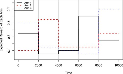
We first consider a piecewise-stationary MAB problem with K = 3 arms, T = 10000 time periods and S = 5 stationary segments (i.e. S−1 = 4 change points). We assume the change points are located evenly over the time horizon, i.e. a change occurs every 2000 time periods. The reward distributions of all arms are assumed to be normal, piecewise-stationary with ${\mu }_k^{\left(i\right)}$ randomly selected from $\{0.05,0.1,0.15,\dots ,0.7\}$ ($i=1,\dots ,S$ and $k=1,\dots ,K$) and having the same standard deviation $\sigma =0.1$. Figure 1 shows the expected rewards for each arm over the time horizon. At each time step t ($t=1,\dots ,T$), there exists a Bernoulli trial $Z_t\in \{0,1\}$ with the probability $P(Z_t=1)=0.025$ to decide whether to use an outlier $Y_t\sim N(2,{\sigma }^2)$ to replace the original reward data at the current moment. That is, the rewards received by the learning agent in this MAB problem are (2) $X_{k,t}=\mathbb{I}\{Z_t=0\}\cdot {\tilde{X}}_{k,t}+\mathbb{I}\{Z_t=1\}\cdot Y_t,$(2) where ${\tilde{X}}_{k,t}\sim N({\mu }_k^{\left(i\right)},{\sigma }^2)$ for $p_{i-1}+1\le t\le p_i$.

Figure 1. Expected rewards for arms in the simulation experiment 1.

We first compare the proposed RCD-UCB with the benchmark method: the M-UCB algorithm (Cao et al., 2019). In the RCD-UCB, we set the tuning parameter D = 200 and consider four different settings for α: 0.01, 0.025, 0.05 and 0.1. According to Theorem 2.2 in this paper and Remark 1 in Cao et al. (2019), we set other tuning parameters as w = 100, $b=15$ and $\gamma =0.19$ for both the RCD-UCB and the M-UCB algorithms. We replicate the simulation experiments 100 times for all algorithms and show the average results. In Figure 2, we display the expected cumulative regrets for the M-UCB and the four RCD-UCB policies (RCD-UCB.S1 to RCD-UCB.S4 using $\alpha =0.01,0.025,0.05$ and 0.1, respectively). It is seen that all the four RCD-UCB policies receive much smaller regrets than the M-UCB algorithm. These four policies perform similarly, where the RCD-UCB.S2 and RCD-UCB.S3 are slightly better in terms of the regret at the end time T .

Figure 2. Expected cumulative regrets for the M-UCB and RCD-UCB with different α values in the simulation experiment 1.

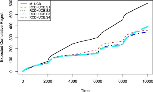
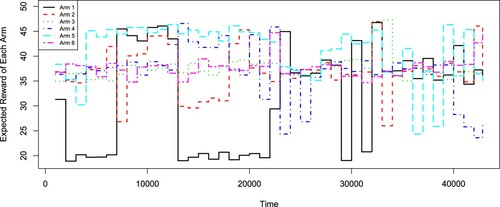
Figure 3. Expected rewards for arms in simulation experiment 2.

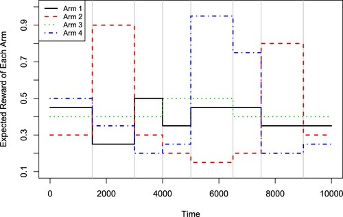
Figure 4. Expected cumulative regrets for M-UCB and RCD-UCB with different α values in the simulation experiment 2.

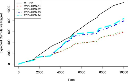
In Table 1, we list the average number of detected change points and its standard deviation for each algorithm among the 100 replications. The M-UCB declares about 7 change points, much larger than its true value of 4. When $\alpha =0.025$ and $\alpha =0.05$, the average numbers of change points detected by the RCD-UCB are close to 4, which explains the superior performance of the RCD-UCB.S2 and RCD-UCB.S3 policies. In the RCD-UCB algorithm, the number of detected change points decreases as α increases. As discussed in Section 2.2, there is a trade-off when choosing the tuning parameter α. Larger α (i.e. larger truncation probability) makes the RCD-UCB more robust towards possibly many outliers, but at the same time makes the algorithm more conservative for identifying change points.

Table 1. Average number (AVE) and standard deviation (SD) of detected change points by each algorithm in the simulation experiment 1.

		RCD-UCB
	M-UCB	$\alpha =0.01$	$\alpha =0.025$	$\alpha =0.05$	$\alpha =0.1$
AVE	6.61	4.82	3.62	3.36	2.98
SD	1.54	1.27	1.02	0.77	0.67

In addition, we compare the RCD-UCB.S2 ($\alpha =0.025$) with the UCB1, the D-UCB and the SW-UCB algorithms. In Table 2, we show the average cumulative regrets at time T and their standard deviations over 100 replications for different algorithms. According to Garivier and Moulines (2011), we set $\gamma =1-0.25\sqrt{(S-1)/T}$ in the D-UCB and $\tau =2\sqrt{2T\log \left(T\right)/(S-1)}$ in the SW-UCB here. From Table 2, we can see that the RCD-UCB gives much smaller (roughly less than a half) T-step cumulative regrets compared to the UCB1, the D-UCB and the SW-UCB algorithms. In addition, we report the average computational time (in seconds) for each algorithm in Table 2. All codes were run in R on a laptop with an Intel 1.60GHz I5 CPU. We can see that all algorithms are very fast for running an MAB problem with T = 10000 time periods. The RCD-UCB algorithm spends a bit more time than the other algorithms, but is still fast enough.

Table 2. Average cumulative regrets $\mathcal{R}\left(T\right)$ (AVE), standard deviations (SD) and computational time in seconds (TIME) for different algorithms in the simulation experiment 1.

	UCB1	D-UCB	SW-UCB	M-UCB	RCD-UCB
Average	1005.26	614.17	764.99	599.17	346.14
SD	53.06	30.52	34.43	62.57	80.80
TIME	0.37	0.39	0.69	0.51	1.91

3.2. Simulation experiment 2

Next, we consider an MAB problem whose reward distributions of all arms are assumed to be Bernoulli, where there are K = 4 arms, T = 10000 time periods and S = 9 stationary segments (i.e. 8 change points). The mean rewards of all arms ${\mu }_k^{\left(i\right)}$ are randomly selected from $\{0.05,0.1,0.15,\dots ,0.95\}$ ($i=1,\dots ,S$ and $k=1,\dots ,K$). Figure 3 shows the expected rewards for each arm over the time horizon. At each time step t $(t=1,\dots ,T)$, there exists a Bernoulli trial $Z_t\in \{0,1\}$ with probability $P(Z_t=1)=0.025$ to decide whether we will use an outlier $Y_t\sim Bernoulli\left(0.99\right)$ to replace the original reward data at the current moment. Thus, the rewards received by the learning agent in this MAB problem are $X_{i,t}=\mathbb{I}\{Z_t=0\}\cdot {\tilde{X}}_{i,t}+\mathbb{I}\{Z_t=1\}\cdot Y_t,$where ${\tilde{X}}_{k,t}\sim Bernoulli\left({\mu }_k^{\left(i\right)}\right)$ for $p_{i-1}+1\le t\le p_i$.

We first compare the proposed RCD-UCB with the benchmark M-UCB. In the RCD-UCB, we set D = 200 and and consider four different settings for α: 0.01, 0.025, 0.05 and 0.1 which are denoted as the RCD-UCB.S1 to RCD-UCB.S4 policies, respectively. Based on Theorem 2.2 in this paper and Remark 1 in Cao et al. (2019), we use w = 100, b = 12 and $\gamma =0.15$ for both the RCD-UCB and the M-UCB algorithms. In Figure 4, we display the expected cumulative regrets for the M-UCB and the four RCD-UCB policies. From Figure 4, it is clear that all the RCD-UCB policies give smaller regrets compared to the M-UCB algorithm. Here, the RCD-UCB.S1 ($\alpha =0.01$) and the RCD-UCB.S2 ($\alpha =0.025$) provide the best performance. We list the average number of detected change points and its standard deviation for each algorithm over the 100 replications in Table 3. Note that the true number of change points here is S−1 = 8. Due to the existence of outliers, the M-UCB declares about 15 change points, which is much larger than the truth. As a comparison, the RCD-UCB.S1 ($\alpha =0.01$) and the RCD-UCB.S2 ($\alpha =0.025$) identify 8.76 and 7.90 change points on average, respectively, which are very close to the truth.

Table 3. Average number (AVE) and standard deviation (SD) of detected change points by each algorithm in the simulation experiment 2.

		RCD-UCB
	M-UCB	$\alpha =0.01$	$\alpha =0.025$	$\alpha =0.05$	$\alpha =0.1$
AVE	14.59	8.76	7.90	3.81	2.92
SD	1.69	1.41	1.35	1.40	1.08

In addition, we compare the RCD-UCB.S2 ($\alpha =0.025$) with the UCB1, the D-UCB and the SW-UCB algorithms in Table 4 which shows the average cumulative regrets at time T, their standard deviations and the average computational time (in seconds) for different algorithms over 100 replications. Here we set $\gamma =1-0.25\sqrt{(S-1)/T}$ for the D-UCB and $\tau =2\sqrt{2T\log \left(T\right)/(S-1)}$ for the SW-UCB according to Garivier and Moulines (2011). From Table 4, it is clear that the RCD-UCB gives much smaller (nearly one half) T-step cumulative regrets compared to the other methods. The computational efficiency of each algorithm here is similar to that in the simulation experiment 1.

Table 4. Average cumulative regrets $\mathcal{R}\left(T\right)$ (AVE), standard deviations (SD) and average computational time in seconds (TIME) for different algorithms in the simulation experiment 2.

	UCB1	D-UCB	SW-UCB	M-UCB	RCD-UCB
AVE	1533.16	1260.24	1192.15	1117.43	603.26
SD	59.74	23.43	27.04	30.9	48.52
TIME	0.36	0.36	0.67	0.46	1.79

3.3. Simulation experiment 3

In this simulation study, we aim to show the proposed RCD-UCB algorithm can still perform well when there are no outliers. Here we consider the same MAB problem in the simulation experiment 1 except that there are no outliers ($Z_t=0$ in Equation (2(2) $X_{k,t}=\mathbb{I}\{Z_t=0\}\cdot {\tilde{X}}_{k,t}+\mathbb{I}\{Z_t=1\}\cdot Y_t,$(2) )). We run the RCD-UCB ($\alpha =0.01$, $\alpha =0.025$, $\alpha =0.05$, $\alpha =0.1$), M-UCB, UCB1, D-UCB and SW-UCB algorithms with the same settings of tuning parameters as those in the simulation experiment 1.

We list the average number of detected change points and its standard deviation for each of the four RCD-UCB algorithms and the M-UCB algorithm over 100 replications in Table 5. It is seen that the numbers of detected change points for all the five algorithms are close to the true value 4. In addition, Table 6 shows the average cumulative regrets at time T and their standard deviations over 100 replications for all the eight algorithms. From Table 6, we can see that the M-UCB algorithm outperforms the UCB1, D-UCB and SW-UCB algorithms. The four RCD-UCB algorithms give similar T-step cumulative regrets as the M-UCB algorithm; while, their standard deviations are slightly larger. This meets our expectation that the proposed RCD-UCB algorithm can also provide desirable performances for cases with no outliers, though they are designed for the cases having outliers.

Table 5. Average number (AVE) and standard deviation (SD) of detected change points by each algorithm in the simulation experiment 3.

		RCD-UCB
	M-UCB	$\alpha =0.01$	$\alpha =0.025$	$\alpha =0.05$	$\alpha =0.1$
AVE	3.93	4.27	3.89	3.83	3.81
SD	0.26	0.77	0.31	0.50	0.37

Table 6. Average cumulative regrets $\mathcal{R}\left(T\right)$ (AVE) and standard deviations (SD) by each algorithm in the simulation experiment 3.

					RCD-UCB
	UCB1	D-UCB	SW-UCB	M-UCB	$\alpha =0.01$	$\alpha =0.025$	$\alpha =0.05$	$\alpha =0.1$
AVE	1012.20	363.48	338.03	292.89	317.38	295.82	286.93	294.28
SD	5.17	5.13	8.99	8.80	23.83	13.44	18.36	12.36

3.4. A real data analysis

We consider a real data example from a metalwork factory in China, which had a task for machining a type of cold-rolled alloy products. There are several parallel production lines machining the same products. The cold-rolled alloys will be annealed, reduced, strengthened and reshaped through the production lines. The elongation rate is one of the key indexes for evaluating the quality of cold-rolled alloy products. It measures the rate of elongation at breaking under the maximum load on the alloy. Larger elongation rate is preferred. In this case study, the original data set includes the elongation rates of the cold-rolled alloys produced by K = 6 parallel production lines over a long time period $T=42842$. At each time t $(t=1,\dots ,T)$, six cold-rolled alloys of the same type from the six production lines are available, and we want to adaptively select one from the six to use. The aim is to maximise the overall elongation rate for the selected products. If we view the elongation rates as rewards, this is an MAB problem with K = 6 arms.

Based on the original data, we group the elongation values of every 1000 successive times for each arm. Figure 5 shows the average rewards for each arm over the time horizon, which ranges from 18.68 to 49.98. All the six arms have non-stationary rewards and there are possibly many change points. Here, unexpected events (e.g. recording errors) may happen which will cause the rewards to be zero. Such outliers can significantly bias the detection of change points in the existing piecewise-stationary algorithms.

Figure 5. Average rewards for arms in the elongation data analysis.

For analysing this real data, we run the proposed RCD-UCB, the benchmark M-UCB, the UCB1, the D-UCB and the SW-UCB algorithms. Specifically, we set the tuning parameters w = 200, b = 80 and $\gamma =0.01$ for the RCD-UCB and the M-UCB algorithms. Based on the simulation experiments in Sections 3.1 and 3.2, we can see $\alpha =0.025$ is a good choice. We set $\alpha =0.025$ and D = 100 in the RCD-UCB. According to Garivier and Moulines (2011), we set the tuning parameters $\gamma =0.99$ and $\tau =1000$ for the D-UCB and SW-UCB, respectively.

Table 7 lists the values of T-step cumulative regrets $\mathcal{R}\left(T\right)$ for all algorithms. It is seen that the proposed RCD-UCB method performs the best among all algorithms and it achieves a nearly 50% reduction in cumulative regrets compared to the M-UCB algorithm. The M-UCB performs slightly better than the D-UCB and SW-UCB algorithms. The UCB1 policy yields the largest regret and is much worse than the others. This is because the UCB1 does not take the non-stationary scenario into consideration. Figure 6 further plots the cumulative regrets for the D-UCB, the SW-UCB, the M-UCB and the RCD-UCB algorithms. From Figure 6, we can also see that the RCD-UCB outperforms all other methods.

Figure 6. Cumulative regrets for different algorithms in the real data analysis.

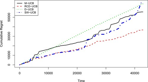
Table 7. Cumulative regrets $\mathcal{R}\left(T\right)$ for different algorithms in the elongation data analysis.

UCB1	D-UCB	SW-UCB	M-UCB	RCD-UCB
251800.60	64408.95	65417.44	55658.80	38674.90

4. Conclusion

In this paper, we consider a general setting of piecewise-stationary MAB problems and propose a RCD-UCB algorithm that is robust to outliers. The RCD-UCB has a simple formulation and is computationally efficient in practice. It can achieve a nearly optimal regret bound on the order of $O\left(\sqrt{SKT\log T}\right)$ under some common assumptions. Most tuning parameters in the RCD-UCB can be specified based on the theoretical results. Yet, if some prior information on the MAB (e.g. the number of piecewise-stationary segments S and the lower bound δ) is unknown in practice, the tuning parameters, including the window width w, the statistical distance threshold b, the exploration probability γ, the truncation probability α and the delay D, need to be chosen based on the practitioner's experience, which is typical in the existing literature (Cao et al., 2019; Liu et al., 2018). Specifically, larger parameter α will make the RCD-UCB more robust towards outliers, but at the same time more likely to miss real change points. Based on the simulation studies in this paper, a choice of $\alpha =0.025$ or 0.05 may be appropriate. Larger parameter D will lead to more stable initial estimates of truncated thresholds, but may also result in longer detection delay. As D is often much smaller than the number of observations between consecutive change points, its impact is usually small in practice. In the current works on the piecewise-stationary MAB problems (Cao et al., 2019; Liu et al., 2018), there lacks a systematic and automatic way to handle tuning parameters when no prior information is available, and it will be an interesting topic for the future research.

Acknowledgments

Wang was supported in part by NSFC (11901199 and 71931004) and Shanghai Sailing Program (19YF1412800). Zhang was supported in part by NSFC (11831008 and 11971171), the National Social Science Foundation Key Program (17ZDA091), and the 111 Project of China (B14019).

The authors thank the editor, the associate editor and the reviewers for their helpful comments.

Disclosure statement

No potential conflict of interest was reported by the authors.

Additional information

Funding

This work was supported by National Natural Science Foundation of China [11901199, 71931004, 11831008, 11971171], Shanghai Sailing Program [19YF1412800], National Social Science Foundation Key Program [17ZDA091] and the 111 Project of China [B14019].

Notes on contributors

Yaping Wang

Dr. Yaping Wang is an assistant professor in school of statistics at East China Normal University.

Zhicheng Peng

Mr. Zhicheng Peng received his master's degree in statistics from East China Normal University in 2020 and is now a researcher at the Ant Group.

Riquan Zhang

Dr. Riquan Zhang is a professor in school of statistics at East China Normal University.

Qian Xiao

Dr. Qian Xiao is an assistant professor in department of statistics at University of Georgia.

Appendices

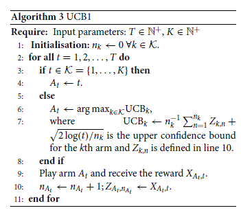
Appendix 1. The UCB1 Algorithm

Auer, Cesa-Bianchi, Freund et al. (2002) proposed an upper confidence bound algorithm, denoted as the UCB1 policy, which becomes a step stone for MAB problems. Following the notations in Section 2.1, we describe the UCB1 policy in Algorithm 3. To balance the exploitation and exploration, the UCB1 algorithm first tries all arms once and then sequentially select the arms with the highest upper bound on its confidence interval, i.e. the UCB1 index (line 7 in Algorithm 3).

Here we briefly summarise its mathematical background. If $X_1,\dots ,X_n$ are independent and 1-subgaussian, we have $P\left(\frac{\sum _{t=1}^n{X}_t}{n}⩾ϵ\right)⩽\mathrm{e}\mathrm{x}\mathrm{p}(-n{ϵ}^2/2).$Let the right-hand side of this equation be δ and we solve for ϵ. Then, we have $P\left(\frac{\sum _{t=1}^n{X}_t}{n}⩾\sqrt{\frac{2}{n}\log \left(\frac{1}{\delta }\right)}\right)⩽\delta .$Following the notations in this paper, when the learner is deciding its action in the time slot t, a good candidate for the largest plausible estimate of the mean for the arm k is $\frac{1}{n_k}\sum _{n=1}^{n_k}{Z}_{k,n}+\sqrt{\frac{2}{n_k}\log \left(\frac{1}{\delta }\right)}.$According to Auer, Cesa-Bianchi, Freund et al. (2002), a good choice for the time dependent δ is $\frac{1}{t}$. Thus, we have the UCB1 index for the kth arm as ${\text{UCB}}_k=n_k^{-1}\sum _{n=1}^{n_k}{Z}_{k,n}+\sqrt{2\log \left(t\right)/n_k}$. Please refer to Auer, Cesa-Bianchi, Freund et al. (2002) for more details on the UCB1 algorithm.

Appendix 2.

Proof of Theorem 2.2

The basic idea of this proof follows the same line of that for classic change detection MAB algorithms. The following lemmas from Cao et al. (2019) are needed and rephrased with our notations.

Lemma A.1

Regret bound in stationary scenarios

Consider a stationary scenario with S = 1, $p_0=0$ and $p_1=T$. Then under Algorithm 2 with parameter w, b and γ, we have that $\mathcal{R}\left(T\right)\le T\cdot P({\tau }_1\le T)+\tilde{C}+\gamma T,$where ${\tau }_1$ is the first detection time and $\tilde{C}=8\sum _{{\mathrm{\Delta }}_k^{\left(1\right)}>0}\log T/{\mathrm{\Delta }}_k^{\left(1\right)}+\left(1+{\pi }^2/3+K\right)\sum _{k=1}^K{\mathrm{\Delta }}_k^{\left(1\right)}.$

Note that the RCD-UCB in Algorithm 2 is stricter than the M-UCB algorithm by Cao et al. (2019) for detecting change points. The probability of raising false alarms in the stationary scenario for the RCD-UCB cannot exceed that for the M-UCB. Thus, the following Lemma A.2 (Lemma 2 of Cao et al. (2019)) holds for the RCD-UCB.

Lemma A.2

Probability of raising false alarms in the stationary scenario

Consider a stationary scenario with S = 1. Then under Algorithm 2 with parameter w<T, b and γ, we have that $P({\tau }_1\le T)<wK\left(1-[1-2\exp (-2b^2/w){]}^{\lfloor T/w\rfloor }\right),$where ${\tau }_1$ is the first detection time.

When L = w + 2D, the uniformity sampling scheme (line 4 of Algorithm 2) guarantees that each arm is sampled at least $w/2+D$ times in any time. Thus, the following Lemma A.3 (Lemma 3 of Cao et al. (2019)) holds, which ensures the detection delay is no more than L/2 with a large probability.

Lemma A.3

Probability of achieving a successful detection with S = 2

Consider a stationary scenario with M = 2 and $L=(w+2D)\lceil K/\gamma \rceil$. Assume that $p_2-p_1>L/2$. For any $({\mu }_1^{\left(1\right)},{\mu }_2^{\left(1\right)},\dots ,{\mu }_K^{\left(1\right)})$ and $({\mu }_1^{\left(2\right)},{\mu }_2^{\left(2\right)},\dots ,{\mu }_K^{\left(2\right)})\in [0,1{]}^K$ satisfying ${\delta }_k^{\left(1\right)}\ge 2b/w+c$ for some $k\in \mathcal{K}$ and c>0, under Algorithm 2, we have that $P(p_1<{\tau }_1\le p_1+L/2\mid p_1>p_2)\ge 1-2\exp (-w{c}^2/4).$

Lemma A.4

Expected detection delay

Consider a piecewise-stationary scenario with M = 2 and $L=(w+2D)\lceil K/\gamma \rceil$. Assume that $p_2-p_1>L/2$. For any $({\mu }_1^{\left(1\right)},{\mu }_2^{\left(1\right)},\dots ,{\mu }_K^{\left(1\right)})$ and $({\mu }_1^{\left(2\right)},{\mu }_2^{\left(2\right)},\dots ,{\mu }_K^{\left(2\right)})\in [0,1{]}^K$ satisfying ${\delta }_k^{\left(1\right)}\ge 2b/w+c$ for some $k\in \mathcal{K}$ and c>0, under Algorithm 2, we have that $\begin{array}{rl}E({\tau }_1-p_1\mid p_1& <{\tau }_1\le p_1+L/2)\\ & \le min\left\{L/2,\lceil b/{\delta }_k^{\left(1\right)}+3\sqrt{w}\cdot \lfloor K/\gamma \rfloor \rceil \right\}/\\ & \times [1-2\exp (-w{c}^2/4\left)\right].\end{array}$

Based on Lemmas A.1–A.4 and Theorem 1 in Cao et al. (2019), it holds that $\begin{array}{rl}\mathcal{R}\left(T\right)& \le \sum _{i=1}^S\left[8\sum _{{\mathrm{\Delta }}_k^{\left(i\right)}>0}\log (p_i-p_{i-1})/{\mathrm{\Delta }}_k^{\left(i\right)}\right.\\ & \times +\left.\left(1+{\pi }^2/3+K\right)\sum _{k=1}^K{\mathrm{\Delta }}_k^{\left(i\right)}\right]\\ & +\gamma T+{\gamma }^{-1}\sum _{i=1}^{S-1}\\ & \times \left(2K\cdot min\{w/2,\lceil b/\underset{k\in \mathcal{K}}{max}{\delta }_k^{\left(i\right)}\rceil +3\sqrt{w}\}\right)+3S.\end{array}$For each $i=1,\dots ,S$, $(8\sum _{{\mathrm{\Delta }}_k^{\left(i\right)}>0}\log (p_i-p_{i-1})/{\mathrm{\Delta }}_k^{\left(i\right)}+(1+{\pi }^2/3+K\left)\sum _{k=1}^K{\mathrm{\Delta }}_k^{\left(i\right)}\right)$ is a classic regret bound for the UCB1 algorithm with time length $p_i-p_{i-1}$. The term $\sum _{i=1}^S[8\sum _{{\mathrm{\Delta }}_k^{\left(i\right)}>0}\log (p_i-p_{i-1})/{\mathrm{\Delta }}_k^{\left(i\right)}+(1+{\pi }^2/3+K\left)\sum _{k=1}^K{\mathrm{\Delta }}_k^{\left(i\right)}\right]$ is of order $O\left(\sqrt{SKT\log T}\right)$ (Cao et al., 2019). The term $\gamma T$ cannot exceed $O\left(\sqrt{SKT\sqrt{\log T+\log K}}\right)=o(SKT\log T)$. The term ${\gamma }^{-1}\sum _{i=1}^{S-1}(2K\cdot min\{w/2,\lceil b/\underset{k\in \mathcal{K}}{max}{\delta }_k^{\left(i\right)}\rceil +3\sqrt{w}\left\}\right)$ cannot exceed $O\left(\sqrt{SKT}\right)=o(SKT\log T)$ and the term $3S$ is of order $O\left(S\right)=o(SKT\log T)$. Thus the result follows.

References

- Alaya-Feki, A. B. H., Moulines, E., & LeCornec, A. (2008). Dynamic spectrum access with non-stationary multi-armed bandit. In 2008 IEEE 9th Workshop on Signal Processing Advances in Wireless Communications. (pp. 416–420). IEEE.
- Allesiardo, R., & Féraud, R. (2015). Exp3 with drift detection for the switching bandit problem. In 2015 IEEE International Conference on Data Science and Advanced Analytics (DSAA) (pp. 1–7). IEEE.
- Auer, P. (2002). Using confidence bounds for exploitation-exploration trade-offs. Journal of Machine Learning Research, 3, 397–422. https://doi.org/10.5555/944919.944941
- Auer, P., Cesa-Bianchi, N., & Fischer, P. (2002). Finite-time analysis of the multiarmed bandit problem. Machine Learning, 47, 235–256. https://doi.org/10.1023/A:1013689704352
- Auer, P., Cesa-Bianchi, N., Freund, Y., & Schapire, R. E. (2002). The nonstochastic multiarmed bandit problem. SIAM Journal on Computing, 32, 48–77. https://doi.org/10.1137/S0097539701398375
- Besbes, O., Gur, Y., & Zeevi, A. (2014). Stochastic multi-armed-bandit problem with non-stationary rewards. In Advances in Neural Information Processing Systems (pp. 199–207). MIT Press.
- Buccapatnam, S., Liu, F., Eryilmaz, A., & Shroff, N. B. (2017). Reward maximization under uncertainty: leveraging side-observations on networks. Journal of Machine Learning Research, 18, 7947–7980. https://doi.org/10.5555/3122009.3242073
- Cao, Y., Wen, Z., Kveton, B., & Xie, Y. (2019). Nearly optimal adaptive procedure with change detection for piecewise-stationary bandit. In Proceedings of Machine Learning Research (pp. 418–427). PMLR.
- Garivier, A., & Moulines, E. (2011). On upper-confidence bound policies for switching bandit problems. In International Conference on Algorithmic Learning Theory (pp. 174–188). Springer.
- Hartland, C., Baskiotis, N., Gelly, S., Sebag, M., & Teytaud, O. (2007). Change point detection and meta-bandits for online learning in dynamic environments. In CAp 2007: 9è Conférence francophone sur l'apprentissage automatique (pp. 237–250). CEPADUES.
- Hinkley, D. V. (1971). Inference about the change-point from cumulative sum tests. Biometrika, 58, 509–523. https://doi.org/10.1093/biomet/58.3.509
- Kaufmann, E., Korda, N., & Munos, R. (2012). Thompson sampling: An asymptotically optimal finite-time analysis. In International Conference on Algorithmic Learning Theory (pp. 199–213). Springer.
- Kocsis, L., & Szepesvári, C. (2006). Discounted UCB. In 2nd PASCAL Challenges Workshop (Vol. 2). http://videolectures.net/pcw06_kocsis_diu/
- Lai, T. L., & Robbins, H. (1985). Asymptotically efficient adaptive allocation rules. Advances in Applied Mathematics, 6, 4–22. https://doi.org/10.1016/0196-8858(85)90002-8
- Lattimore, T., & Szepesvári, C. (2020). Bandit algorithms. Cambridge University Press.
- Li, S., Karatzoglou, A., & Gentile, C. (2016). Collaborative filtering bandits. In Proceedings of the 39th International ACM SIGIR Conference on Research and Development in Information Retrieval (pp. 539–548). New York, NY: Association for Computing Machinery.
- Liu, F., Lee, J., & Shroff, N. (2018). A change-detection based framework for piecewise-stationary multi-armed bandit problem. In Proceedings of the AAAI Conference on Artificial Intelligence. Palo Alto, CA: AAAI Press.
- Mellor, J., & Shapiro, J. (2013). Thompson sampling in switching environments with Bayesian online change detection. In Artificial Intelligence and Statistics (pp. 442–450). Springer.
- Srivastava, V., Reverdy, P., & Leonard, N. E. (2014). Surveillance in an abruptly changing world via multiarmed bandits. In 53rd IEEE Conference on Decision and Control (pp. 692–697). IEEE.
- Thompson, W. R. (1933). On the likelihood that one unknown probability exceeds another in view of the evidence of two samples. Biometrika, 25, 285–294. https://doi.org/10.1093/biomet/25.3-4.285
- Yu, J. Y., & Mannor, S. (2009). Piecewise-stationary bandit problems with side observations. In Proceedings of the 26th Annual International Conference on Machine Learning (pp. 1177–1184). New York, NY: Association for Computing Machinery.