Empirical likelihood inference in autoregressive models with time-varying variances

Abstract

This paper develops the empirical likelihood ($\mathrm{E}\mathrm{L}$) inference procedure for parameters in autoregressive models with the error variances scaled by an unknown nonparametric time-varying function. Compared with existing methods based on non-parametric and semi-parametric estimation, the proposed test statistic avoids estimating the variance function, while maintaining the asymptotic chi-square distribution under the null. Simulation studies demonstrate that the proposed $\mathrm{E}\mathrm{L}$ procedure (a) is more stable, i.e., depending less on the change points in the error variances, and (b) gets closer to the desired confidence level, than the traditional test statistic.

Keywords:

• Empirical likelihood
• autoregressive model
• unconditional heteroscedasticity
• stable test

1. Introduction

In the literature of the macroeconomics and financial applications, the assumption of heteroscedasticity in many time series models revealed the facts that ignoring the issue of heteroscedasticity often leads to the inefficient estimation and unreliable inference. Thus, heteroscedasticity has been focused mainly on the effect of violations of homoscedasticity, usually in two forms, ‘conditional heteroscedasticity’ and ‘unconditional heteroscedasticity’.

Non-constant volatility will be identified by ‘conditional heteroscedasticity’, when future periods of high and low volatility cannot be identified. Bollerslev (1986) and Engle (1982) proposed ARCH or GARCH models and provided the efficient estimation of the mean function by quasi-maximum likelihood based on other adaptive procedures. More complicated GARCH models had been proposed to allow for conditional heteroscedasticity, for instance, varying coefficient GARCH models (see Polzehl & Spokoiny, 2006) and spline GARCH models (see Engle & Rangel, 2008). The time-varying volatility is often used to describe the conditional heteroscedasticity. Drees and Starica (2002) and Starica (2003) made use of a non-stationary framework to analyse time series of S&P 500 returns, and found that this approach outperformed the GARCH-type models.

‘Unconditional heteroscedasticity’ will be used, when variables that have identifiable seasonal variability, such as electricity usage, are discussed. Hansen (1995) considered the linear regression model with deterministically trending regressors only, in which the error is an $\mathrm{A}\mathrm{R}\left(p\right)$ process scaled by a continuous function of time. Nesting autoregressive model is also a special case when the conditional error variance of the model is a function of a covariate that has a form of a nearly integrated stochastic process with no deterministic drift. For the constant coefficient autoregressive model with time-varying variances ($\mathrm{A}\mathrm{R}\mathrm{T}\mathrm{V}$) which will be discussed in this article, Phillips and Xu (2006) utilised the ordinary least squares method and the nonparametric estimation of the variance function to provide three heteroscedasticity-robust test statistics, and proved their asymptotic standard normal distributions. Xu and Phillips (2008) proposed the heteroscedasticity-robust adaptive estimation for $\mathrm{A}\mathrm{R}\mathrm{T}\mathrm{V}$. Meanwhile, performances of methods in Phillips and Xu (2006) and Xu and Phillips (2008) relied on appropriately selecting the bandwidth used in the non-parametric function estimation.

Motivated from the ‘empirical likelihood’ ($\mathrm{E}\mathrm{L}$) approach, this article aims to develop a test statistic which is more stable, namely, depending less on the change points in the error variances, and avoiding the problem of selecting the bandwidth. In the literature, the $\mathrm{E}\mathrm{L}$ approach was introduced by Owen (1988), Owen (1990) and Owen (1991) to construct confidence intervals in a nonparametric setting, which can be seen in Owen (2001). Since an $\mathrm{E}\mathrm{L}$ approach possesses nonparametric properties, the distribution for the data is not required to be specified, and meanwhile more efficient estimates of the parameters can be yielded. The $\mathrm{E}\mathrm{L}$ approach allows data to decide the shape of confidence regions without estimating the variance of the test statistic, and also is Bartlett correctable in DiCiccio et al. (1991). The $\mathrm{E}\mathrm{L}$ approach has been applied to various situations, such as generalised linear models in Kolaczyk (1994), local linear smoother in Chen and Qin (2000), partially linear models in Shi and Lau (2000), parametric and semi-parametric models in multi response regression in Chen and Ingrid (2009); linear regression with censored data in Zhou and Li (2008), plug-in estimates of nuisance parameters in estimating equations in the context of survival analysis in Li and Wang (2003) and Qin and Jing (2001), heteroscedastic partially linear models in Lu (2009); GARCH models in Chan and Ling (2006); variable selection in Han et al. (2013) and Variyath and Chen (2010); analysis of longitudinal data in Qiu and Wu (2015). Qin and Lawless (1994) linked the $\mathrm{E}\mathrm{L}$ with finitely many estimating equations, which served as finitely many equality constraints. To the best of our knowledge, there is no existing published work in the literature using the $\mathrm{E}\mathrm{L}$ approach in the constant coefficient autoregressive models with time-varying variances. This article will also consider the constant coefficient autoregressive models with time-varying innovation variance by using the $\mathrm{E}\mathrm{L}$ approach.

The remainder of the paper proceeds as follows. Section 2 describes the autoregressive model with time-varying variances and discusses main assumptions. Section 3 reviews the existing methods. Section 4 develops the empirical likelihood inference procedure with theoretical guarantees. Section 5 conducts simulation studies to evaluate the finite sample performance of the proposed method when compared with alternative methods. Section 6 briefly concludes. Technical details and proofs of the main results are relegated to Appendix.

2. Autoregressive model with time-varying variances

The constant coefficient autoregressive model with time-varying variances is described as follows, (1) $\begin{array}{rl}{Y}_t& ={\text{β}}_0+{\text{β}}_1{Y}_{t-1}+{\text{β}}_2{Y}_{t-2}+\cdots +{\text{β}}_p{Y}_{t-p}+u_t\\ & ={\mathit{X}}_{t-1}^{\mathrm{\top }}{\text{β}}_{\mathrm{o}}+u_t,\end{array}$(1) (2) $\begin{array}{rl}{u}_t& ={\sigma }_t{ϵ}_t,t=1,\dots ,T,\end{array}$(2) where $\mathrm{\top }$ denotes transpose, ${\mathit{X}}_{t-1}=(1,Y_{t-1},\dots ,Y_{t-p}{)}^{\mathrm{\top }}\in {\mathbb{R}}^{p+1}$ is the vector of covariates, and ${\text{β}}_{\mathrm{o}}=({\text{β}}_0,{\text{β}}_1,\dots ,{\text{β}}_p{)}^{\mathrm{\top }}\in {\mathbb{R}}^{p+1}$ is the true parameter vector of interest, with ${\text{β}}_p\ne 0$, and the lag order p finite and known. We assume that $\left\{{\sigma }_t\right\}$ is a deterministic sequence of time t, satisfying (3) ${\sigma }_t=g\left(t/T\right),$(3) and $\left\{{ϵ}_t\right\}$ is a martingale difference sequence with respect to ${\mathcal{F}}_t$, where ${\mathcal{F}}_t=\sigma ({ϵ}_s:s\le t)$ is the σ-field generated by $\{{ϵ}_s:s\le t\}$ with $\mathrm{E}({ϵ}_t^2\mid {\mathcal{F}}_{t-1})=1$, $\mathrm{a}.\mathrm{s}.$, for all t. Thus, the conditional variance of $\left\{u_t\right\}$ is fully characterised by the multiplicative factor ${\sigma }_t$ in (2(2) $\begin{array}{rl}{u}_t& ={\sigma }_t{ϵ}_t,t=1,\dots ,T,\end{array}$(2) ), i.e., (4) $\mathrm{E}\left(u_t^2|{\mathcal{F}}_{t-1}\right)={\sigma }_t^2=g^2\left(t/T\right),\mathrm{a}.\mathrm{s}..$(4) Suppose that the data are generated from models (1(1) $\begin{array}{rl}{Y}_t& ={\text{β}}_0+{\text{β}}_1{Y}_{t-1}+{\text{β}}_2{Y}_{t-2}+\cdots +{\text{β}}_p{Y}_{t-p}+u_t\\ & ={\mathit{X}}_{t-1}^{\mathrm{\top }}{\text{β}}_{\mathrm{o}}+u_t,\end{array}$(1) )–(2(2) $\begin{array}{rl}{u}_t& ={\sigma }_t{ϵ}_t,t=1,\dots ,T,\end{array}$(2) ), and we observe a sample containing T + p observations, denoted by $\{Y_{-p+1},Y_{-p+2},\dots ,Y_0,Y_1,\dots ,Y_T\}$. The main goals are to make inferences about the true parameter vector ${\text{β}}_{\mathrm{o}}$ in models (1(1) $\begin{array}{rl}{Y}_t& ={\text{β}}_0+{\text{β}}_1{Y}_{t-1}+{\text{β}}_2{Y}_{t-2}+\cdots +{\text{β}}_p{Y}_{t-p}+u_t\\ & ={\mathit{X}}_{t-1}^{\mathrm{\top }}{\text{β}}_{\mathrm{o}}+u_t,\end{array}$(1) )–(2(2) $\begin{array}{rl}{u}_t& ={\sigma }_t{ϵ}_t,t=1,\dots ,T,\end{array}$(2) ), i.e., testing the null hypothesis, (5) $H_0:{\text{β}}_{\mathrm{o}}={\mathit{b}}_0,$(5) where ${\mathit{b}}_0=(b_{0,0},b_{0,1},\dots ,b_{0,p})\in {\mathbb{R}}^{p+1}$, and constructing a confidence region for ${\text{β}}_{\mathrm{o}}$.

Section 4 will present our proposed empirical likelihood inference, after Section 3 describes the estimation methods in Phillips and Xu (2006).

To facilitate the discussion of main results and comparison with related existing methods, the following conditions provided in Phillips and Xu (2006); Xu and Phillips (2008) are considered.

Conditions

1. $g(\cdot )$ in (3(3) ${\sigma }_t=g\left(t/T\right),$(3) ) and (4(4) $\mathrm{E}\left(u_t^2|{\mathcal{F}}_{t-1}\right)={\sigma }_t^2=g^2\left(t/T\right),\mathrm{a}.\mathrm{s}..$(4) ) is a measurable and strictly positive function on the interval $(0,1]$ such that $0<\underset{r\in (0,1]}{inf}g\left(r\right)\le \underset{r\in (0,1]}{sup}g\left(r\right)<\mathrm{\infty }$, and $g\left(r\right)$ satisfies a Lipschitz condition except at a finite number of points of discontinuity;

2. Suppose that L is the lag operator. Then $0=1-{\text{β}}_{1}L-{\text{β}}_2{L}^2-\cdots -{\text{β}}_p{L}^p$ has all roots outside the unit circle;

3. $\left\{{ϵ}_t\right\}$ satisfies $\mathrm{E}({ϵ}_t\mid {\mathcal{F}}_{t-1})=0$, and $\mathrm{E}\left({ϵ}_t^2|{\mathcal{F}}_{t-1}\right)=1$, $\mathrm{a}.\mathrm{s}.$, for all t;

4. $\underset{t}{sup}\mathrm{E}\left(|{ϵ}_t^{4\nu }|\right)<\mathrm{\infty }$ for some $\nu >1$.

Remark 2.1

1. In condition (A1), the function g is integrable on the interval $(0,1]$ to any finite order. For brevity, we write ${\int }_0^1{g}^m\left(x\right)\mathrm{d}x$ as $\int g^m$ for any finite positive integer $m\ge 1$.

2. Condition (A2) satisfies the stability conditions which, for a constant $g(\cdot )$ and homoskedastic $\left\{{ϵ}_t\right\}$, would ensure that $\left\{Y_t\right\}$ is stationary or asymptotically covariance-stationary. Under condition (A2), the mean μ of $Y_t$ is given by $\mu =\frac{{\text{β}}_0}{1-{\text{β}}_1-\cdots -{\text{β}}_p},$ and $Y_t$ has the Wold representation, $Y_t=\mu +\sum _{i=1}^{\mathrm{\infty }}{\alpha }_i{u}_{t-i},$ where $\left\{{\alpha }_i\right\}$ satisfies that ${\alpha }_i-{\text{β}}_1{\alpha }_{i-1}-\cdots -{\text{β}}_p{\alpha }_{i-p}=0,\mathrm{a}\mathrm{s}i>0,$ and $\sum _{i=1}^{\mathrm{\infty }}|{\alpha }_i|<\mathrm{\infty }$. Define Ω to be the matrix with the $(i,j)$-th element ${\gamma }_{|i-j|}$, where ${\gamma }_k=\sum _{i=0}^{\mathrm{\infty }}{\alpha }_i{\alpha }_{i+k}<\mathrm{\infty }$.

3. Condition (A3) ensures that $\left\{{ϵ}_t\right\}$ is a martingale difference sequence and, at the same time, stipulates $\mathrm{E}(u_t^2\mid {\mathcal{F}}_{t-1})=g^2\left(t/T\right)$ doesn't depend on the past events, in other words, models (1(1) $\begin{array}{rl}{Y}_t& ={\text{β}}_0+{\text{β}}_1{Y}_{t-1}+{\text{β}}_2{Y}_{t-2}+\cdots +{\text{β}}_p{Y}_{t-p}+u_t\\ & ={\mathit{X}}_{t-1}^{\mathrm{\top }}{\text{β}}_{\mathrm{o}}+u_t,\end{array}$(1) )–(2(2) $\begin{array}{rl}{u}_t& ={\sigma }_t{ϵ}_t,t=1,\dots ,T,\end{array}$(2) ) are unconditional heteroscedastic.

3. Existing methods

Regarding the estimation of ${\text{β}}_{\mathrm{o}}$ in models (1(1) $\begin{array}{rl}{Y}_t& ={\text{β}}_0+{\text{β}}_1{Y}_{t-1}+{\text{β}}_2{Y}_{t-2}+\cdots +{\text{β}}_p{Y}_{t-p}+u_t\\ & ={\mathit{X}}_{t-1}^{\mathrm{\top }}{\text{β}}_{\mathrm{o}}+u_t,\end{array}$(1) )–(2(2) $\begin{array}{rl}{u}_t& ={\sigma }_t{ϵ}_t,t=1,\dots ,T,\end{array}$(2) ), Phillips and Xu (2006) reviewed the ordinary least squares ($\mathrm{O}\mathrm{L}\mathrm{S}$) estimator $\widehat{\text{β}}$, and showed that under the stated conditions, as $T\to \mathrm{\infty }$, (6) $\begin{array}{rl}\sqrt{T}(\widehat{\text{β}}-{\text{β}}_{\mathrm{o}})& ={\left(\frac{1}{T}\sum _{t=1}^T{\mathit{X}}_{t-1}^{\mathrm{\top }}{\mathit{X}}_{t-1}\right)}^{-1}\\ & \times \left(\frac{1}{\sqrt{T}}\sum _{t=1}^T{\mathit{X}}_{t-1}^{\mathrm{\top }}{ϵ}_t\right)\stackrel{\mathcal{D}}{\to }N(\mathbf{0},\mathrm{\Lambda }),\end{array}$(6) where $\stackrel{\mathcal{D}}{\to }$ stands for converges in distribution, $\mathrm{\Lambda }={\mathrm{\Omega }}_1^{-1}{\mathrm{\Omega }}_2{\mathrm{\Omega }}_1^{-1}$, ${\mathrm{\Omega }}_1$ and ${\mathrm{\Omega }}_2$ are defined as the $(p+1)\times (p+1)$ matrices, (7) $\begin{array}{rl}{\mathrm{\Omega }}_1& =\left(\begin{array}{cc}1& \mu {\mathbf{l}}_p^{\mathrm{\top }}\\ \mu {\mathbf{l}}_p& {\mu }^2+(\int g^2)\mathrm{\Omega }\end{array}\right),\\ {\mathrm{\Omega }}_2& =\left(\begin{array}{cc}(\int g^2)& \mu (\int g^2){\mathbf{l}}_p^{\mathrm{\top }}\\ \mu (\int g^2){\mathbf{l}}_p& {\mu }^2(\int g^2)+(\int g^4)\mathrm{\Omega }\end{array}\right),\end{array}$(7) ${\mathbf{l}}_p=(1,\dots ,1{)}^{\mathrm{\top }}\in {\mathbb{R}}^p$ is a vector of ones, and μ and Ω are as defined in Remark 2.1.

Since g is typically unknown, the asymptotic covariance matrix Λ in (6(6) $\begin{array}{rl}\sqrt{T}(\widehat{\text{β}}-{\text{β}}_{\mathrm{o}})& ={\left(\frac{1}{T}\sum _{t=1}^T{\mathit{X}}_{t-1}^{\mathrm{\top }}{\mathit{X}}_{t-1}\right)}^{-1}\\ & \times \left(\frac{1}{\sqrt{T}}\sum _{t=1}^T{\mathit{X}}_{t-1}^{\mathrm{\top }}{ϵ}_t\right)\stackrel{\mathcal{D}}{\to }N(\mathbf{0},\mathrm{\Lambda }),\end{array}$(6) ) must be estimated and this can be done in several ways. First, by applying the weighted sum of squared $\mathrm{O}\mathrm{L}\mathrm{S}$ residuals using kernel smoothing, originally proposed by Nadaraya (1964) and Watson (1964) for estimation of regression functions, they proposed the consistent estimator of the function $g^2\left(r\right)$ non-parametrically for $r\in [0,1]$, (8) ${\hat{g}}^2\left(r\right)=\sum _{t=1}^T{w}_{r,t}{\hat{u}}_t^2,$(8) where ${\hat{u}}_t=Y_t-{\mathit{X}}_{t-1}^{\mathrm{\top }}\widehat{\text{β}}$ is the $\mathrm{O}\mathrm{L}\mathrm{S}$ residual and the weights $w_{r,t}$, $t=1,\dots ,T$, are defined as (9) $w_{r,t}={\left\{\sum _{t=1}^{T}K\left(\frac{\left[Tr\right]-t}{T{h}_T}\right)\right\}}^{-1}K\left(\frac{\left[Tr\right]-t}{T{h}_T}\right),$(9) where the kernel function $K(\cdot ):\mathbb{R}\mapsto [0,\mathrm{\infty })$ is assumed to satisfy $0\le K\left(z\right)\le C_1<\mathrm{\infty }$ uniformly in z and ${\int }_{-\mathrm{\infty }}^{\mathrm{\infty }}K\left(z\right)\mathrm{d}z<C_2<\mathrm{\infty },$ for some constant $C_1$ and $C_2$; $h_T$ is a bandwidth parameter depending on T. The selection of bandwidth parameter $h_T$ uses the cross-validation procedure, i.e., minimises the averaged squared prediction errors (see Wong, 1983), (10) $\mathrm{C}\mathrm{V}\left(b\right)=\frac{1}{T}\sum _{s=1}^T\{{\hat{u}}_s^2-{\hat{g}}_{-s}^2(s/T){\}}^2,$(10) with respect to b, where ${\hat{g}}_{-s}^2\left(r\right)=\sum _{t=1,t\ne s}{w}_{r,t}{\hat{u}}_t^2.$ Phillips and Xu (2006) suggested the following three consistent estimators of the asymptotic covariance matrix Λ when g is unknown.

• The first estimator of the asymptotic covariance matrix is (11) $\begin{array}{rl}{\hat{\mathrm{\Lambda }}}_1& =T{\left(\sum _{t=1}^T{\mathit{X}}_{t-1}{\mathit{X}}_{t-1}^{\mathrm{\top }}\right)}^{-1}\left(\sum _{t=1}^T{\hat{u}}_t^2{\mathit{X}}_{t-1}{\mathit{X}}_{t-1}^{\mathrm{\top }}\right)\\ & \times {\left(\sum _{t=1}^T{\mathit{X}}_{t-1}{\mathit{X}}_{t-1}^{\mathrm{\top }}\right)}^{-1}.\end{array}$(11)

• The second estimator of the asymptotic covariance matrix is (12) ${\hat{\mathrm{\Lambda }}}_2={\hat{\mathrm{\Omega }}}_1^{-1}\left(\sum _{t=1}^T{\hat{u}}_t^2{\mathit{X}}_{t-1}{\mathit{X}}_{t-1}^{\mathrm{\top }}\right){\hat{\mathrm{\Omega }}}_1^{-1},$(12) where the matrix ${\hat{\mathrm{\Omega }}}_1$ is defined as $\begin{array}{r}{\hat{\mathrm{\Omega }}}_1=\left(\begin{array}{cc}1& \hat{\mu }{\mathbf{l}}_p^{\mathrm{\top }}\\ \hat{\mu }{\mathbf{l}}_p& {\hat{\mu }}^2+\left(T^{-1}{\displaystyle \sum _{t=1}^T{\hat{u}}_t^2}\right)\hat{\mathrm{\Omega }}\end{array}\right),\end{array}$ where $\hat{\mu }$ and $\hat{\mathrm{\Omega }}$ correspond to replacing ${\text{β}}_{\mathrm{o}}$, in the expressions of μ and Ω in Remark 2.1, with $\widehat{\text{β}}$.

• The third estimator of the asymptotic covariance matrix is (13) ${\hat{\mathrm{\Lambda }}}_3={\hat{\mathrm{\Omega }}}_1^{-1}{\tilde{\mathrm{\Omega }}}_2{\hat{\mathrm{\Omega }}}_1^{-1},$(13) where the matrix ${\hat{\mathrm{\Omega }}}_2$ is defined as $\begin{array}{r}{\tilde{\mathrm{\Omega }}}_2=\left(\begin{array}{cc}\int {\hat{g}}^2& \hat{\mu }(\int {\hat{g}}^2){\mathbf{l}}_p^{\mathrm{\top }}\\ \hat{\mu }(\int {\hat{g}}^2){\mathbf{l}}_p& {\hat{\mu }}^2(\int {\hat{g}}^2)+(\int {\hat{g}}^4)\hat{\mathrm{\Omega }}\end{array}\right).\end{array}$

Based on the above three estimators ${\hat{\mathrm{\Lambda }}}_j$ of the true covariance matrix Λ, Phillips and Xu (2006) constructed three test statistics $t_j$, j = 1, 2, 3, for the true parameter vector ${\text{β}}_{\mathrm{o}}$, stated as follows.

Lemma 3.1

Theorem 2(ii) in Phillips and Xu (2006)

Assume that $\widehat{\text{β}}$ is the $\mathrm{O}\mathrm{L}\mathrm{S}$ estimator of ${\text{β}}_{\mathrm{o}}$. Then, under the above assumptions and null hypothesis (5(5) $H_0:{\text{β}}_{\mathrm{o}}={\mathit{b}}_0,$(5) ), it follows that (14) $t_j=\frac{\sqrt{T}({\widehat{\text{β}}}_k-b_{0,k})}{\left(\right({\hat{\mathrm{\Lambda }}}_j{)}_{kk}{)}^{1/2}}\stackrel{\mathcal{D}}{\to }N(0,1),\mathrm{a}\mathrm{s}T\to \mathrm{\infty },$(14) where $({\hat{\mathrm{\Lambda }}}_j{)}_{kk}$ is the $(k,k)$-th element of the matrix ${\hat{\mathrm{\Lambda }}}_j$, j = 1, 2, 3, defined in (11(11) $\begin{array}{rl}{\hat{\mathrm{\Lambda }}}_1& =T{\left(\sum _{t=1}^T{\mathit{X}}_{t-1}{\mathit{X}}_{t-1}^{\mathrm{\top }}\right)}^{-1}\left(\sum _{t=1}^T{\hat{u}}_t^2{\mathit{X}}_{t-1}{\mathit{X}}_{t-1}^{\mathrm{\top }}\right)\\ & \times {\left(\sum _{t=1}^T{\mathit{X}}_{t-1}{\mathit{X}}_{t-1}^{\mathrm{\top }}\right)}^{-1}.\end{array}$(11) ), (12(12) ${\hat{\mathrm{\Lambda }}}_2={\hat{\mathrm{\Omega }}}_1^{-1}\left(\sum _{t=1}^T{\hat{u}}_t^2{\mathit{X}}_{t-1}{\mathit{X}}_{t-1}^{\mathrm{\top }}\right){\hat{\mathrm{\Omega }}}_1^{-1},$(12) ) and (13(13) ${\hat{\mathrm{\Lambda }}}_3={\hat{\mathrm{\Omega }}}_1^{-1}{\tilde{\mathrm{\Omega }}}_2{\hat{\mathrm{\Omega }}}_1^{-1},$(13) ), respectively.

Hence, a large sample level $100(1-\alpha )\mathrm{\%}$ confidence region for ${\text{β}}_o$ based on the above Normal approximation (14(14) $t_j=\frac{\sqrt{T}({\widehat{\text{β}}}_k-b_{0,k})}{\left(\right({\hat{\mathrm{\Lambda }}}_j{)}_{kk}{)}^{1/2}}\stackrel{\mathcal{D}}{\to }N(0,1),\mathrm{a}\mathrm{s}T\to \mathrm{\infty },$(14) ) is given by (15) $\begin{array}{rl}{\mathrm{\Re }}_{j,\alpha }& =\{\mathit{b}:T(\widehat{\text{β}}-\mathit{b}{)}^{\mathrm{\top }}\\ & \times \left[\mathrm{d}\mathrm{i}\mathrm{a}\mathrm{g}\right\{({\hat{\mathrm{\Lambda }}}_j{)}_{k,k},k=0,1,\dots ,p\}{]}^{-1}(\widehat{\text{β}}-\mathit{b})\\ & \le {\chi }_{p;1-\alpha }^2\},\end{array}$(15) where $\mathrm{d}\mathrm{i}\mathrm{a}\mathrm{g}\left\{\right({\hat{\mathrm{\Lambda }}}_j{)}_{k,k},k=0,1,\dots ,p\}$ is the main diagonal matrix of ${\hat{\mathrm{\Lambda }}}_j$, j = 1, 2, 3, and ${\chi }_{p;1-\alpha }^2$ denotes the $100(1-\alpha )$th quantile of the chi-square distribution ${\chi }_p^2$ with p degrees of freedom.

4. Proposed method

In terms of the practical performance of the three tests $t_j$ in (14(14) $t_j=\frac{\sqrt{T}({\widehat{\text{β}}}_k-b_{0,k})}{\left(\right({\hat{\mathrm{\Lambda }}}_j{)}_{kk}{)}^{1/2}}\stackrel{\mathcal{D}}{\to }N(0,1),\mathrm{a}\mathrm{s}T\to \mathrm{\infty },$(14) ), however, simulation results reveal two major issues arising from the estimation of the asymptotic covariance matrix and the selection of the bandwidth. In order to solve these problems, the proposed empirical likelihood approach will be applied to test parameters in models (1(1) $\begin{array}{rl}{Y}_t& ={\text{β}}_0+{\text{β}}_1{Y}_{t-1}+{\text{β}}_2{Y}_{t-2}+\cdots +{\text{β}}_p{Y}_{t-p}+u_t\\ & ={\mathit{X}}_{t-1}^{\mathrm{\top }}{\text{β}}_{\mathrm{o}}+u_t,\end{array}$(1) )–(2(2) $\begin{array}{rl}{u}_t& ={\sigma }_t{ϵ}_t,t=1,\dots ,T,\end{array}$(2) ).

To construct an empirical likelihood function, the estimation equations will be defined by means of, (16) ${\mathit{W}}_t\left(\mathit{b}\right)={\mathit{X}}_{t-1}\cdot (Y_t-{\mathit{X}}_{t-1}^{\mathrm{\top }}\mathit{b}),$(16) for a generic model parameter $\mathit{b}\in {\mathbb{R}}^{p+1}$. According to condition (A3), we have that $\begin{array}{rl}& \mathrm{E}\left({\mathit{W}}_t\right({\text{β}}_{\mathrm{o}}\left)\right)\\ & =\mathrm{E}\left({\mathit{X}}_{t-1}g\right(t/T\left){ϵ}_t\right)=g\left(t/T\right)\mathrm{E}\left({\mathit{X}}_{t-1}{ϵ}_t\right)=\mathbf{0}\end{array}$ holds for the true parameter vector ${\text{β}}_{\mathrm{o}}$. Based on (16(16) ${\mathit{W}}_t\left(\mathit{b}\right)={\mathit{X}}_{t-1}\cdot (Y_t-{\mathit{X}}_{t-1}^{\mathrm{\top }}\mathit{b}),$(16) ), we define the empirical likelihood for the parameter $\mathit{b}$ by $L\left(\mathit{b}\right)=sup\{\prod _{t=1}^T{q}_t:\sum _{t=1}^T{q}_t=1,\sum _{t=1}^T{q}_t{\mathit{W}}_t(\mathit{b})=\mathbf{0}\}.$ By using the Lagrange multiplier, we have ${\hat{q}}_t\left(\mathit{b}\right)=\frac{1}{T}\{1+{\hat{\mathit{\lambda }}}^{\mathrm{\top }}{\mathit{W}}_t(\mathit{b}){\}}^{-1},t=1,\dots ,T,$ where $\hat{\mathit{\lambda }}=\hat{\mathit{\lambda }}\left(\mathit{b}\right)\in {\mathbb{R}}^{p+1}$ is the solution of equations, (17) $\frac{1}{T}\sum _{t=1}^T\frac{{\mathit{W}}_t\left(\mathit{b}\right)}{1+{\hat{\mathit{\lambda }}}^{\mathrm{\top }}{\mathit{W}}_t\left(\mathit{b}\right)}=\mathbf{0}.$(17) We also note that $\prod _{t=1}^T{q}_t$, subject to constraints $q_t\ge 0$ and $\sum _{t=1}^T{q}_t=1$, attains its maximum $(1/T{)}^T$ at $q_t=1/T$. Thus, the empirical likelihood ratio at $\mathit{b}$ is defined by $\mathrm{E}\mathrm{L}\mathrm{R}\left(\mathit{b}\right)=\prod _{t=1}^T\left\{{\hat{q}}_t\right(\mathit{b})T{\}}^{-1}=\prod _{t=1}^T\{1+{\hat{\mathit{\lambda }}}^{\mathrm{\top }}{\mathit{W}}_t\left(\mathit{b}\right)\}.$ Taking the log transformation of the above equation, we get the corresponding empirical log-likelihood ratio, (18) $\ell \left(\mathit{b}\right)=2\sum _{t=1}^T\log \{1+{\hat{\mathit{\lambda }}}^{\mathrm{\top }}{\mathit{W}}_t(\mathit{b}\left)\right\}.$(18) In addition, Theorem 4.1 below provides the asymptotic null distribution of $\ell \left({\text{β}}_{\mathrm{o}}\right)$.

Theorem 4.1

Assume that conditions (A1)–(A4) hold. Then, under the null hypothesis (5(5) $H_0:{\text{β}}_{\mathrm{o}}={\mathit{b}}_0,$(5) ), the limiting distribution of $\ell \left({\text{β}}_{\mathrm{o}}\right)$ is the chi-square distribution with p degrees of freedom, i.e., (19) $\ell \left({\text{β}}_{\mathrm{o}}\right)\stackrel{\mathcal{D}}{\to }{\chi }_p^2,\mathrm{a}\mathrm{s}T\to \mathrm{\infty }.$(19)

According to Theorem 4.1, the empirical likelihood ratio confidence interval for the true value ${\text{β}}_{\mathrm{o}}$ can be constructed as follows: (20) ${\mathrm{\Re }}_{\mathrm{E}\mathrm{L},\alpha }=\{\mathit{b}:\ell (\mathit{b})\le {\chi }_{p;1-\alpha }^2\},$(20) where ${\chi }_{p;1-\alpha }^2$ is defined below (15(15) $\begin{array}{rl}{\mathrm{\Re }}_{j,\alpha }& =\{\mathit{b}:T(\widehat{\text{β}}-\mathit{b}{)}^{\mathrm{\top }}\\ & \times \left[\mathrm{d}\mathrm{i}\mathrm{a}\mathrm{g}\right\{({\hat{\mathrm{\Lambda }}}_j{)}_{k,k},k=0,1,\dots ,p\}{]}^{-1}(\widehat{\text{β}}-\mathit{b})\\ & \le {\chi }_{p;1-\alpha }^2\},\end{array}$(15) ). Combined with (20(20) ${\mathrm{\Re }}_{\mathrm{E}\mathrm{L},\alpha }=\{\mathit{b}:\ell (\mathit{b})\le {\chi }_{p;1-\alpha }^2\},$(20) ), Theorem 4.1 implies Corollary 4.1.

Corollary 4.1

Under the conditions of Theorem 4.1, $\text{P}({\text{β}}_{\mathrm{o}}\in {\mathrm{\Re }}_{\mathrm{E}\mathrm{L},\alpha })\to 1-\alpha ,\mathrm{a}\mathrm{s}T\to \mathrm{\infty }.$

5. Simulation evaluation

In this section, simulation studies are conducted to compare the finite sample performance of five methods described in Sections 3–4:

• Ordinary least squares without the heteroscedasticity correction ($\mathrm{O}\mathrm{L}\mathrm{S}$),

• $t_1$, $t_2$, $t_3$,

• the proposed empirical likelihood ($\mathrm{E}\mathrm{L}$) procedure.

The zero-mean $\mathrm{A}\mathrm{R}\left(1\right)$ with the time-varying variance is considered as follows: $Y_t={\text{β}}_{0,1}{Y}_{t-1}+g\left(t/T\right){ϵ}_t,$ where $\left\{{ϵ}_t\right\}\stackrel{\mathrm{i}.\mathrm{i}.\mathrm{d}.}{\sim }N(0,1)$. The kernel function $K(\cdot )$ is the standard Normal density function, $K\left(x\right)=\frac{1}{\sqrt{2\pi }}\exp (-\frac{x^2}{2}),-\mathrm{\infty }<x<\mathrm{\infty },$ and the bandwidth parameter is selected by the cross-validation criterion (10(10) $\mathrm{C}\mathrm{V}\left(b\right)=\frac{1}{T}\sum _{s=1}^T\{{\hat{u}}_s^2-{\hat{g}}_{-s}^2(s/T){\}}^2,$(10) ). We consider $H_0:{\text{β}}_{0,1}={\text{β}}_1$ with known values of ${\text{β}}_1$.

Three kinds of the variance functions $g^2\left(r\right)$ are considered in the following simulations: a single abrupt point model, two abrupt points model, continuous function variance model as follows.

Model 1: A single abrupt point model, $g^2\left(r\right)={\sigma }_0^2+({\sigma }_1^2-{\sigma }_0^2){\mathrm{I}}_{\{r\ge \kappa \}},r\in [0,1].$ Model 1 corresponds to the case of a single abrupt change of the error variance from ${\sigma }_0^2$ to ${\sigma }_1^2$ at time $\left[\kappa T\right]$, where κ is the break point within the value set $\{0.1,0.5,0.9\}$. The ratio of post-break and pre-break standard deviations $\delta ={\sigma }_1/{\sigma }_0$ is within the value set $\{0.2,1,5\}$ where ${\sigma }_0=1$.

Model 2: Two abrupt points model, $\begin{array}{rl}{g}^2\left(r\right)& ={\sigma }_0^2+({\sigma }_1^2-{\sigma }_0^2){\mathrm{I}}_{\{{\kappa }_0<r\le {\kappa }_1\}}+({\sigma }_2^2-{\sigma }_0^2){\mathrm{I}}_{\{{\kappa }_1<r\}},\\ & r\in [0,1].\end{array}$ Model 2 corresponds to the case of two abrupt points model which has the change of the error variance from ${\sigma }_0^2$ to ${\sigma }_1^2$ and ${\sigma }_1^2$ to ${\sigma }_2^2$. The time break points $({\kappa }_0,{\kappa }_1)$ take the values $(0.1,0.9)$; $({\sigma }_0^2,{\sigma }_1^2,{\sigma }_2^2)$ are from the set $\left\{\right(0.2,5,0.2),(5,0.2,5\left)\right\}$.

Model 3: Continuous function variance model, $g^2\left(r\right)={\sigma }_0^2+({\sigma }_1^2-{\sigma }_0^2)r^m,r\in [0,1].$ Model 3 considers that the variance of the errors is the continuous function from ${\sigma }_0^2$ to ${\sigma }_1^2$. We suppose m to be within the value set $\{1,2\}$ and $\delta ={\sigma }_1/{\sigma }_0$ within the value set $\{0.2,5\}$ where ${\sigma }_0^2=1$.

Model 1 and Model 3 are the same as in Cavaliere (2004), Cavaliere and Taylor (2007) and Phillips and Xu (2006). Simulations are done when the parameter of interest ${\text{β}}_1$ increases on the set $\{0.1,0.5,0.9\}$, and the nominal size is $5\mathrm{\%}$. The sample size T is from $\{60,200\}$ respectively. The number of Monte Carlo replications is 5000.

Simulation results include two parts. The first part displayed in Tables 1, 2 and 3 assesses the rejection rates of five methods under the null hypothesis.

Table 1. Comparison of the rejection rates of five methods in Model 1 for ${\text{β}}_1\in \{0.1,0.5,0.9\}$, $\kappa \in \{0.1,0.5,0.9\}$, $\delta \in \{0.2,1,5\}$ and the sample size $T\in \{60,200\}$, based on 5000 replications.

			T = 60					T = 200
${\text{β}}_1$	κ	δ	$\mathrm{O}\mathrm{L}\mathrm{S}$	$t_1$	$t_2$	$t_3$	EL	$\mathrm{O}\mathrm{L}\mathrm{S}$	$t_1$	$t_2$	$t_3$	$\mathrm{E}\mathrm{L}$
0.1	0.1	0.2	0.3386	0.1428	0.0560	0.1010	0.1724	0.3804	0.0972	0.0676	0.0840	0.0958
		1	0.0558	0.0692	0.0560	0.0450	0.0658	0.0436	0.0510	0.0476	0.0414	0.0492
		5	0.0644	0.0712	0.0628	0.0520	0.0654	0.0594	0.0558	0.0536	0.0464	0.0530
	0.5	0.2	0.1480	0.0812	0.0486	0.0506	0.0750	0.1528	0.0636	0.0524	0.0590	0.0610
		5	0.1526	0.0846	0.0682	0.0642	0.0798	0.1422	0.0608	0.0566	0.0528	0.0550
	0.9	0.2	0.0666	0.0716	0.0520	0.0432	0.0700	0.0588	0.0552	0.0498	0.0468	0.0524
		5	0.3400	0.1632	0.1624	0.1258	0.1712	0.3780	0.0966	0.0940	0.0754	0.0956
0.5	0.1	0.2	0.3146	0.1278	0.1066	0.1004	0.1632	0.3826	0.0924	0.0886	0.0884	0.0940
		1	0.0528	0.0666	0.0762	0.0514	0.0646	0.0494	0.0554	0.0648	0.0540	0.0536
		5	0.0622	0.0682	0.0822	0.0548	0.0644	0.0606	0.0564	0.0682	0.0560	0.0542
	0.5	0.2	0.1452	0.0766	0.0830	0.0608	0.0752	0.1600	0.0650	0.0692	0.0640	0.0614
		5	0.1396	0.0792	0.1014	0.0748	0.0736	0.1416	0.0572	0.0664	0.0552	0.0540
	0.9	0.2	0.0654	0.0692	0.0720	0.0474	0.0658	0.0630	0.0590	0.0636	0.0558	0.0574
		5	0.3232	0.1462	0.1952	0.1388	0.1638	0.3760	0.0948	0.01154	0.0796	0.0970
0.9	0.1	0.2	0.1954	0.0836	0.2328	0.1144	0.1278	0.3038	0.0664	0.1926	0.0914	0.0730
		1	0.0544	0.0650	0.1950	0.1172	0.0600	0.0548	0.0584	0.1160	0.0756	0.0560
		5	0.0596	0.0656	0.2086	0.1286	0.0604	0.0638	0.0570	0.1212	0.0792	0.0512
	0.5	0.2	0.1250	0.0724	0.2288	0.1334	0.0714	0.1478	0.0654	0.1492	0.0980	0.0636
		5	0.1442	0.0768	0.2552	0.1632	0.0728	0.1412	0.0580	0.1578	0.0982	0.0560
	0.9	0.2	0.0618	0.0646	0.1844	0.1116	0.0618	0.0650	0.0588	0.1162	0.0808	0.0568
		5	0.2778	0.1136	0.3962	0.2100	0.1454	0.3402	0.0780	0.2406	0.1108	0.0862

Table 2. Comparison of the rejection rates of five methods in Model 2 for ${\text{β}}_1\in \{0.1,0.5,0.9\}$, $[{\kappa }_0,{\kappa }_1]=[0.1,0.9]$, $[{\sigma }_0,{\sigma }_1,{\sigma }_2]\in \left\{\right[0.2,5,0.2],[5,0.2,5\left]\right\}$ and the sample size $T\in \{60,200\}$, based on 5000 replications.

				T = 60					T = 200
${\text{β}}_1$	${\sigma }_0$	${\sigma }_1$	${\sigma }_2$	$\mathrm{O}\mathrm{L}\mathrm{S}$	$t_1$	$t_2$	$t_3$	$\mathrm{E}\mathrm{L}$	$\mathrm{O}\mathrm{L}\mathrm{S}$	$t_1$	$t_2$	$t_3$	$\mathrm{E}\mathrm{L}$
0.1	0.2	5	0.2	0.0520	0.0888	0.0278	0.0234	0.0712	0.0438	0.0546	0.0360	0.0340	0.0496
	5	0.2	5	0.0570	0.0712	0.0628	0.0492	0.0664	0.0444	0.0504	0.0480	0.0418	0.0488
0.5	0.2	5	0.2	0.0514	0.0762	0.0408	0.0320	0.0714	0.0510	0.0570	0.0472	0.0426	0.0540
	5	0.2	5	0.0548	0.0704	0.0812	0.0498	0.0544	0.0480	0.0558	0.0650	0.0548	0.0540
0.9	0.2	5	0.2	0.0550	0.0698	0.1302	0.0806	0.0640	0.0552	0.0566	0.0976	0.0676	0.0536
	5	0.2	5	0.0522	0.0644	0.1996	0.1178	0.0598	0.0540	0.0598	0.1172	0.0752	0.0572

Table 3. Comparison of the rejection rates of five methods in Model 3 for ${\text{β}}_1\in \{0.1,0.5,0.9\}$, $m\in \{1,2\}$, $\delta \in \{0.2,5\}$ and the sample size $t\in \{60,200\}$, based on 5000 replications.

			T = 60					T = 200
${\text{β}}_1$	m	δ	$\mathrm{O}\mathrm{L}\mathrm{S}$	$t_1$	$t_2$	$t_3$	$\mathrm{E}\mathrm{L}$	$\mathrm{O}\mathrm{L}\mathrm{S}$	$t_1$	$t_2$	$t_3$	$\mathrm{E}\mathrm{L}$
0.1	1	0.2	0.0820	0.0812	0.0604	0.0446	0.0826	0.0820	0.0550	0.0476	0.0518	0.0546
		5	0.0780	0.0688	0.0624	0.0542	0.0632	0.0828	0.0582	0.0564	0.0540	0.0566
	2	0.2	0.0756	0.0784	0.0548	0.0498	0.0628	0.0676	0.0544	0.0482	0.0464	0.0520
		5	0.1200	0.0854	0.0778	0.0688	0.0716	0.1200	0.0620	0.0596	0.0582	0.0586
0.5	1	0.2	0.0800	0.0772	0.0780	0.0474	0.0782	0.0912	0.0620	0.0674	0.0620	0.0620
		5	0.0872	0.0800	0.0926	0.0670	0.0682	0.0804	0.0560	0.0674	0.0564	0.0544
	2	0.2	0.0766	0.0728	0.0728	0.0550	0.0656	0.0752	0.0602	0.0666	0.0598	0.0600
		5	0.1196	0.0806	0.0104	0.0844	0.0718	0.1212	0.0604	0.0734	0.0640	0.0590
0.9	1	0.2	0.0672	0.06640	0.1972	0.1112	0.0644	0.0830	0.0642	0.1268	0.0822	0.0606
		5	0.0789	0.0688	0.2238	0.1356	0.0578	0.0854	0.0564	0.1322	0.0850	0.0558
	2	0.2	0.0652	0.0676	0.1866	0.1166	0.0562	0.0732	0.0640	0.1198	0.0818	0.0628
		5	0.1258	0.0826	0.2572	0.1686	0.0668	0.1196	0.0622	0.1500	0.0958	0.0608

The second part includes Figures 1–3 to evaluate the rejection rates of methods $\mathrm{O}\mathrm{L}\mathrm{S}$, $t_1$, $t_2$, $t_3$ and $\mathrm{E}\mathrm{L}$ as the parameter ${\text{β}}_1$ under the alternatives increases.

Figure 1. The relationship between the rejection rates of $\mathrm{O}\mathrm{L}\mathrm{S}$, $t_1$, $t_2$, $t_3$, $\mathrm{E}\mathrm{L}$ and the true coefficient ${\text{β}}_1$ in Model 1 $($a single abrupt point model$)$. The abrupt point $\kappa =0.1$, $\delta =0.2$. The true parameter ${\text{β}}_1$ increases gradually from 0.1 to 0.9. (a) The sample T = 60; (b) the sample T = 200.

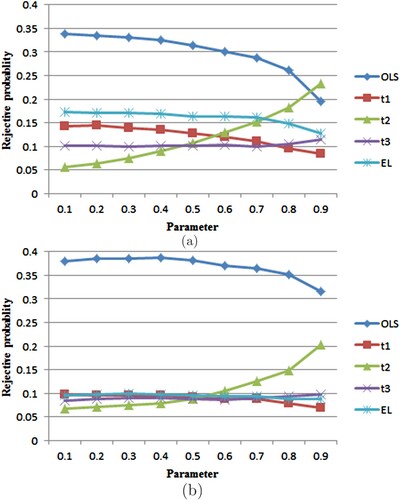
From these simulations, we draw the following conclusions.

1. First, the $\mathrm{O}\mathrm{L}\mathrm{S}$-based test is the inefficient and unreliable test under the heteroscedastic innovations. From Table 1, the $\mathrm{O}\mathrm{L}\mathrm{S}$-based test overrejects overwhelmingly the null hypothesis when the null is true, and has the largest distorted size under $(\kappa ,\delta )\in \left\{\right(0.1,0.2),(0.9,5\left)\right\}$. In addition, the distorted size doesn't reduce except for the homoscedastic innovations with the increasing sample size which is also shown in Figures 1 and 3. From Table 2, the $\mathrm{O}\mathrm{L}\mathrm{S}$-based test has better performance than Table 1, however, the rejection rate reduces as the sample size increases. The results of the $\mathrm{O}\mathrm{L}\mathrm{S}$-based test in Table 3 are similar to those in Table 1.

2. Second, the performance of $t_2$ and $t_3$ depends on the numerical value of the true parameter and the pattern of the variance function. From Figures 1, 2, 3, an interesting phenomenon can be found that the rejection rates of $t_2$ and $t_3$ are likely to be an increasing function of the parameter and grow bigger as ${\text{β}}_1>0.5$. The rejection rate of $t_2$ is far greater than the nominal size $5\mathrm{\%}$ when the numerical value of the parameter is close to unity, namely ${\text{β}}_1=0.9$. In particular, it is easy to see that $t_2$ and $t_3$ overaccept the null hypothesis when the parameter is less than or equal to $5\mathrm{\%}$ when ${\text{β}}_1<0.5$. On the contrary, $t_2$ and $t_3$ overreject the null hypothesis when ${\text{β}}_1>0.9$. It also has the similar conclusions from Tables 1–3. So both $t_2$ and $t_3$ aren't the stable test for the $\mathrm{A}\mathrm{R}\mathrm{T}\mathrm{V}$ model.

3. Third, both $\mathrm{E}\mathrm{L}$ and $t_1$ are the stable tests for the $\mathrm{A}\mathrm{R}\mathrm{T}\mathrm{V}$ model and $\mathrm{E}\mathrm{L}$ outperforms $t_1$. From Tables 1–3, we can find that $\mathrm{E}\mathrm{L}$ and $t_1$ overreject the null hypothesis when the null is true. From Figures 1–3, the rejection rate of $\mathrm{E}\mathrm{L}$ is almost a horizontal line and is closer to the nominal level $5\mathrm{\%}$ than $t_1$ except Figure 1(a) when the sample size is 60. When the sample size is 200, EL's rejection rate is nearly a nominal size of $5\mathrm{\%}$ and doesn't depend on the numerical value of the parameters even if the true value of β is close to unity $({\text{β}}_1=0.9)$. $\mathrm{E}\mathrm{L}$ has the smallest size distortion overall and avoids correcting the variance. The simulation results generally support the asymptotic results. $\mathrm{E}\mathrm{L}$ is more stable and has better performance than $\mathrm{O}\mathrm{L}\mathrm{S}$, $t_1$, $t_2$, $t_3$ for testing the parameters of $\mathrm{A}\mathrm{R}\mathrm{T}\mathrm{V}$. So $\mathrm{E}\mathrm{L}$ seems to be the better choice.

Figure 2. The relationship between the rejection rates of $\mathrm{O}\mathrm{L}\mathrm{S}$, $t_1$, $t_2$, $t_3$, $\mathrm{E}\mathrm{L}$ and the true coefficient ${\text{β}}_1$ in Model 2 $($two abrupt points model$)$. The abrupt points ${\kappa }_1=0.1$, ${\kappa }_2=0.9$, $[{\sigma }_0,{\sigma }_1,{\sigma }_2]=[0.2,5,0.2]$. The true parameter ${\text{β}}_1$ increases gradually from 0.1 to 0.9. (a) The sample T = 60; (b) the sample T = 200.

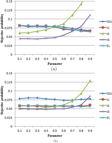
Figure 3. The relationship between the rejection rates of $\mathrm{O}\mathrm{L}\mathrm{S}$, $t_1$, $t_2$, $t_3$, $\mathrm{E}\mathrm{L}$ corresponding to the true coefficient ${\text{β}}_1$ in Model 3 $($continuous function variance model$)$, and m = 1, $\delta =0.2$. The true parameter ${\text{β}}_1$ increases gradually from 0.1 to 0.9. (a) The sample T = 60; (b) the sample T = 200.

6. Conclusion

This article focuses on the empirical likelihood approach for autoregressive models with error terms scaled by an unknown nonparametric time-varying function. The empirical likelihood ratio test statistic avoids estimating the unknown variance function, in the presence of heteroscedastic error terms. The results of simulations of three different models show that the empirical likelihood is more stable than the other four test statistics. In addition, some extensions include improving the efficiency of statistic based on the different equations, and locating the abrupt time points when they exist.

Acknowledgments

The authors thank the editor, Prof. Jun Shao, and two anonymous reviewers for helpful comments. Yu Han was supported by the Scientific Research Foundation of Jilin Education (JJKH20200102KJ). The work of C. Zhang was partially supported by U.S. National Science Foundation grants DMS-2013486 and DMS-1712418, and provided by the University of Wisconsin-Madison Office of the Vice Chancellor for Research and Graduate Education with funding from the Wisconsin Alumni Research Foundation.

Disclosure statement

No potential conflict of interest was reported by the author(s).

Additional information

Funding

The authors thank the editor, Prof. Jun Shao, and two anonymous reviewers for helpful comments. Yu Han was supported by the Scientific Research Foundation of Jilin Education [grant number JJKH20200102KJ]. The work of C. Zhang was partially supported by U.S. National Science Foundation [grant numbers DMS-2013486 and DMS-1712418], and provided by the University of Wisconsin-Madison Office of the Vice Chancellor for Research and Graduate Education with funding from the Wisconsin Alumni Research Foundation.

Notes on contributors

Yu Han

Yu Han, received Ph.D. degree in mathematical statistics from Jilin University in 2012. He is currently an associate research fellow in the Educational Supervision and Evaluation Center of Northeast Electrical Power University. His current research interests are Time Series Analysis, Non-parametric and semi-parametric estimation & inference. He worked at Department of Statistics, Wisconsin University-Madison between 2013 and 2014 as a visiting scholar. He has published 12 papers. He has accomplished 3 projects as a principle investigator and as a participator. One was accomplished, and two are ongoing.

Chunming Zhang

Chunming Zhang is Professor of Statistics at the University of Wisconsin-Madison. Her research interests range from statistical learning and data mining, statistical methods with applications to imaging data, neuroinformatics and bioinformatics, multiple testing, large-scale simultaneous inference and applications, statistical methods in financial econometrics, non- and semi-parametric estimation and inference, to functional and longitudinal data analysis.

Appendix. Proofs of main results

Before proving Theorem 4.1, we first show Lemmas A.1–A.2. To simplify notations, we denote $\hat{\mathit{\lambda }}=\hat{\mathit{\lambda }}\left({\text{β}}_{\mathrm{o}}\right)$ and ${\mathit{W}}_t={\mathit{W}}_t\left({\text{β}}_{\mathrm{o}}\right)$.

Lemma A.1

Assume that conditions (A1)–(A4) hold. Then (A1) $\begin{array}{rl}& \frac{1}{\sqrt{T}}\sum _{t=1}^T{\mathit{W}}_t\stackrel{\mathcal{D}}{\to }N(\mathbf{0},{\mathrm{\Omega }}_2),\end{array}$(A1) (A2) $\begin{array}{rl}& \frac{1}{T}\sum _{t=1}^T{\mathit{W}}_t{\mathit{W}}_t^{\mathrm{\top }}\stackrel{\mathrm{P}}{\to }{\mathrm{\Omega }}_2,\end{array}$(A2) where $\stackrel{\mathrm{P}}{\to }$ denotes converges in probability.

Proof.

According to Phillips and Xu (2006) (Lemma 1(iii) –(iv)), the proof of Lemma A.1 completes.

Lemma A.2

Assume that conditions (A1)–(A3) hold. Then $\hat{\mathit{\lambda }}=O_{\text{P}}\left(T^{-1/2}\right).$

Proof.

From (17(17) $\frac{1}{T}\sum _{t=1}^T\frac{{\mathit{W}}_t\left(\mathit{b}\right)}{1+{\hat{\mathit{\lambda }}}^{\mathrm{\top }}{\mathit{W}}_t\left(\mathit{b}\right)}=\mathbf{0}.$(17) ), we have $\mathbf{0}=\frac{1}{T}\sum _{t=1}^T{\mathit{W}}_t-\frac{1}{T}\sum _{t=1}^T\frac{{\mathit{W}}_t{\mathit{W}}_t^{\mathrm{\top }}}{1+{\hat{\mathit{\lambda }}}^{\mathrm{\top }}{\mathit{W}}_t}\hat{\mathit{\lambda }}.$ By (A1(A1) $\begin{array}{rl}& \frac{1}{\sqrt{T}}\sum _{t=1}^T{\mathit{W}}_t\stackrel{\mathcal{D}}{\to }N(\mathbf{0},{\mathrm{\Omega }}_2),\end{array}$(A1) ) of Lemma 3.1, $\begin{array}{rl}& \frac{\Vert \hat{\mathit{\lambda }}{\Vert }_2}{1+\Vert \hat{\mathit{\lambda }}{\Vert }_2\underset{t}{max}\Vert {\mathit{W}}_t{\Vert }_2}\Vert \frac{1}{T}\sum _{t=1}^T{\mathit{W}}_t{\mathit{W}}_t^{\mathrm{\top }}\Vert \\ & \le {\Vert \frac{1}{T}\sum _{t=1}^T{\mathit{W}}_t\Vert }_2=O_{\text{P}}\left(T^{-1/2}\right).\end{array}$ According to conditions (A1) and (A4), we have $\mathrm{E}\left(|Y_t{|}^{4\nu }\right)<\mathrm{\infty }$ for some $\nu >1$, and then (A3) $\begin{array}{rl}& \underset{t}{max}\Vert {\mathit{W}}_t{\Vert }_2\\ & =\underset{t}{max}\Vert {\mathit{X}}_{t-1}(Y_t-{\text{β}}_{\mathrm{o}}^{\mathrm{\top }}{\mathit{X}}_{t-1}){\Vert }_2=\underset{t}{max}\Vert {\mathit{X}}_{t-1}{u}_t{\Vert }_2\\ & =\underset{t}{max}\Vert {\mathit{X}}_{t-1}g\left(t/T\right){ϵ}_t{\Vert }_2=o_{\text{P}}\left(T^{\frac{1}{4\nu }}\right).\end{array}$(A3) From (A2(A2) $\begin{array}{rl}& \frac{1}{T}\sum _{t=1}^T{\mathit{W}}_t{\mathit{W}}_t^{\mathrm{\top }}\stackrel{\mathrm{P}}{\to }{\mathrm{\Omega }}_2,\end{array}$(A2) ) of Lemma A.1 and a similar argument used in Owen (1991), the proof of Lemma A.2 is completed.

Proof of Theorem 4.1.

Noticing that if ${\text{β}}_{\mathrm{o}}$ is the true parameters, applying Taylor's expansion to (18(18) $\ell \left(\mathit{b}\right)=2\sum _{t=1}^T\log \{1+{\hat{\mathit{\lambda }}}^{\mathrm{\top }}{\mathit{W}}_t(\mathit{b}\left)\right\}.$(18) ), we have (A4) $\begin{array}{rl}\ell \left({\text{β}}_{\mathrm{o}}\right)& =2\sum _{t=1}^T\log (1+{\hat{\mathit{\lambda }}}^{\mathrm{\top }}{\mathit{W}}_t)\\ & =2\sum _{t=1}^T\{{\hat{\mathit{\lambda }}}^{\mathrm{\top }}{\mathit{W}}_t-\frac{1}{2}({\hat{\mathit{\lambda }}}^{\mathrm{\top }}{\mathit{W}}_t{)}^2\}+r_T,\end{array}$(A4) where $r_T$, in probability, satisfies the following inequality in light of Lemma A.1 (A2(A2) $\begin{array}{rl}& \frac{1}{T}\sum _{t=1}^T{\mathit{W}}_t{\mathit{W}}_t^{\mathrm{\top }}\stackrel{\mathrm{P}}{\to }{\mathrm{\Omega }}_2,\end{array}$(A2) ) and Lemma A.2 for some constant C>0, $\begin{array}{rl}|r_T|& \le C\sum _{t=1}^T|{\hat{\mathit{\lambda }}}^{\mathrm{\top }}{\mathit{W}}_t{|}^3\\ & \le C\Vert \hat{\mathit{\lambda }}{\Vert }_2^3\underset{1\le t\le T}{max}\Vert {\mathit{W}}_t{\Vert }_2\sum _{t=1}^T\Vert {\mathit{W}}_t{\Vert }_2^2=o_{\text{P}}\left(1\right).\end{array}$ By Lemma A.1 (A2(A2) $\begin{array}{rl}& \frac{1}{T}\sum _{t=1}^T{\mathit{W}}_t{\mathit{W}}_t^{\mathrm{\top }}\stackrel{\mathrm{P}}{\to }{\mathrm{\Omega }}_2,\end{array}$(A2) ), Lemma A.2 and similar arguments as above, we have (A5) $\sum _{t=1}^T\frac{({\hat{\mathit{\lambda }}}^{\mathrm{\top }}{\mathit{W}}_t{)}^3}{1+{\hat{\mathit{\lambda }}}^{\mathrm{\top }}{\mathit{W}}_t}=o_{\text{P}}\left(1\right).$(A5) By (17(17) $\frac{1}{T}\sum _{t=1}^T\frac{{\mathit{W}}_t\left(\mathit{b}\right)}{1+{\hat{\mathit{\lambda }}}^{\mathrm{\top }}{\mathit{W}}_t\left(\mathit{b}\right)}=\mathbf{0}.$(17) ), we obtain (A6) $\begin{array}{rl}0& =\sum _{t=1}^T\frac{{\hat{\mathit{\lambda }}}^{\mathrm{\top }}{\mathit{W}}_t}{1+{\hat{\mathit{\lambda }}}^{\mathrm{\top }}{\mathit{W}}_t}=\sum _{t=1}^T\left({\hat{\mathit{\lambda }}}^{\mathrm{\top }}{\mathit{W}}_t\right)-\sum _{t=1}^T({\hat{\mathit{\lambda }}}^{\mathrm{\top }}{\mathit{W}}_t{)}^2\\ & +\sum _{t=1}^T\frac{({\hat{\mathit{\lambda }}}^{\mathrm{\top }}{\mathit{W}}_t{)}^3}{1+{\hat{\mathit{\lambda }}}^{\mathrm{\top }}{\mathit{W}}_t}.\end{array}$(A6) By (A5(A5) $\sum _{t=1}^T\frac{({\hat{\mathit{\lambda }}}^{\mathrm{\top }}{\mathit{W}}_t{)}^3}{1+{\hat{\mathit{\lambda }}}^{\mathrm{\top }}{\mathit{W}}_t}=o_{\text{P}}\left(1\right).$(A5) ) and (A6(A6) $\begin{array}{rl}0& =\sum _{t=1}^T\frac{{\hat{\mathit{\lambda }}}^{\mathrm{\top }}{\mathit{W}}_t}{1+{\hat{\mathit{\lambda }}}^{\mathrm{\top }}{\mathit{W}}_t}=\sum _{t=1}^T\left({\hat{\mathit{\lambda }}}^{\mathrm{\top }}{\mathit{W}}_t\right)-\sum _{t=1}^T({\hat{\mathit{\lambda }}}^{\mathrm{\top }}{\mathit{W}}_t{)}^2\\ & +\sum _{t=1}^T\frac{({\hat{\mathit{\lambda }}}^{\mathrm{\top }}{\mathit{W}}_t{)}^3}{1+{\hat{\mathit{\lambda }}}^{\mathrm{\top }}{\mathit{W}}_t}.\end{array}$(A6) ), we obtain (A7) $\sum _{t=1}^T\left({\hat{\mathit{\lambda }}}^{\mathrm{\top }}{\mathit{W}}_t\right)=\sum _{t=1}^T({\hat{\mathit{\lambda }}}^{\mathrm{\top }}{\mathit{W}}_t{)}^2+o_{\text{P}}(1).$(A7) Again by (17(17) $\frac{1}{T}\sum _{t=1}^T\frac{{\mathit{W}}_t\left(\mathit{b}\right)}{1+{\hat{\mathit{\lambda }}}^{\mathrm{\top }}{\mathit{W}}_t\left(\mathit{b}\right)}=\mathbf{0}.$(17) ), we obtain $\begin{array}{rl}\mathbf{0}& =\sum _{t=1}^T\frac{{\mathit{W}}_t}{1+{\hat{\mathit{\lambda }}}^{\mathrm{\top }}{\mathit{W}}_t}=\sum _{t=1}^T{\mathit{W}}_t\{1-{\hat{\mathit{\lambda }}}^{\mathrm{\top }}{\mathit{W}}_t+\frac{({\hat{\mathit{\lambda }}}^{\mathrm{\top }}{\mathit{W}}_t{)}^2}{1+{\hat{\mathit{\lambda }}}^{\mathrm{\top }}{\mathit{W}}_t}\}\\ & =\sum _{t=1}^T{\mathit{W}}_t-\sum _{t=1}^T\left({\mathit{W}}_t{\mathit{W}}_t^{\mathrm{\top }}\right)\hat{\mathit{\lambda }}+\sum _{t=1}^T\frac{{\mathit{W}}_t({\hat{\mathit{\lambda }}}^{\mathrm{\top }}{\mathit{W}}_t{)}^2}{1+{\hat{\mathit{\lambda }}}^{\mathrm{\top }}{\mathit{W}}_t}.\end{array}$ By Lemma A.1 and (A3(A3) $\begin{array}{rl}& \underset{t}{max}\Vert {\mathit{W}}_t{\Vert }_2\\ & =\underset{t}{max}\Vert {\mathit{X}}_{t-1}(Y_t-{\text{β}}_{\mathrm{o}}^{\mathrm{\top }}{\mathit{X}}_{t-1}){\Vert }_2=\underset{t}{max}\Vert {\mathit{X}}_{t-1}{u}_t{\Vert }_2\\ & =\underset{t}{max}\Vert {\mathit{X}}_{t-1}g\left(t/T\right){ϵ}_t{\Vert }_2=o_{\text{P}}\left(T^{\frac{1}{4\nu }}\right).\end{array}$(A3) ), we have $\begin{array}{rl}& \frac{1}{T}\sum _{t=1}^T{\Vert \frac{{\mathit{W}}_t({\hat{\mathit{\lambda }}}^{\mathrm{\top }}{\mathit{W}}_t{)}^2}{1+{\hat{\mathit{\lambda }}}^{\mathrm{\top }}{\mathit{W}}_t}\Vert }_2\\ & \le C\Vert {\hat{\mathit{\lambda }}}^2{\Vert }_2\underset{t}{max}\Vert {\mathit{W}}_t{\Vert }_2\frac{1}{T}\sum _{t=1}^T\Vert {\mathit{W}}_t{\Vert }_2^2=o_{\text{P}}\left(T^{-1/2}\right).\end{array}$ Thus, we have $\begin{array}{rl}\hat{\mathit{\lambda }}& ={\left(\sum _{t=1}^T{\mathit{W}}_t{\mathit{W}}_t^{\mathrm{\top }}\right)}^{-1}\sum _{t=1}^T{\mathit{W}}_t+{\left(\frac{1}{T}\sum _{t=1}^T{\mathit{W}}_t{\mathit{W}}_t^{\mathrm{\top }}\right)}^{-1}\\ & \times \left\{\frac{1}{T}\sum _{t=1}^T\frac{{\mathit{W}}_t({\hat{\mathit{\lambda }}}^{\mathrm{\top }}{\mathit{W}}_t{)}^2}{1+{\hat{\mathit{\lambda }}}^{\mathrm{\top }}{\mathit{W}}_t}\right\}\\ & ={\left(\sum _{t=1}^T{\mathit{W}}_t{\mathit{W}}_t^{\mathrm{\top }}\right)}^{-1}\sum _{t=1}^T{\mathit{W}}_t+o_{\text{P}}\left(T^{-1/2}\right).\end{array}$ By substituting $\hat{\mathit{\lambda }}$ of the above equation into (A4(A4) $\begin{array}{rl}\ell \left({\text{β}}_{\mathrm{o}}\right)& =2\sum _{t=1}^T\log (1+{\hat{\mathit{\lambda }}}^{\mathrm{\top }}{\mathit{W}}_t)\\ & =2\sum _{t=1}^T\{{\hat{\mathit{\lambda }}}^{\mathrm{\top }}{\mathit{W}}_t-\frac{1}{2}({\hat{\mathit{\lambda }}}^{\mathrm{\top }}{\mathit{W}}_t{)}^2\}+r_T,\end{array}$(A4) ) and (A7(A7) $\sum _{t=1}^T\left({\hat{\mathit{\lambda }}}^{\mathrm{\top }}{\mathit{W}}_t\right)=\sum _{t=1}^T({\hat{\mathit{\lambda }}}^{\mathrm{\top }}{\mathit{W}}_t{)}^2+o_{\text{P}}(1).$(A7) ), we have $\begin{array}{rl}\ell \left({\text{β}}_{\mathrm{o}}\right)& =\sum _{t=1}^T{\hat{\mathit{\lambda }}}^{\mathrm{\top }}{\mathit{W}}_t{\mathit{W}}_t^{\mathrm{\top }}\hat{\mathit{\lambda }}+o_{\text{P}}\left(1\right)\\ & ={\left(T^{-1/2}\sum _{t=1}^T{\mathit{W}}_t\right)}^{\mathrm{\top }}{\left(T^{-1}\sum _{t=1}^T{\mathit{W}}_t{\mathit{W}}_t^{\mathrm{\top }}\right)}^{-1}\\ & \times \left(T^{-1/2}\sum _{t=1}^T{\mathit{W}}_t\right)+o_{\text{P}}\left(1\right).\end{array}$ The proof of Theorem 4.1 is completed by using Lemma A.1.

References

- Bollerslev, T. (1986). Generalized autoregressive conditional heteroskedasticity. Journal of Econometrics, 31, 307–327. https://doi.org/https://doi.org/10.1016/0304-4076(86)90063-1
- Cavaliere, G. (2004). Unit root tests under time-varying variance shifts. Econometric Reviews, 23, 259–292. https://doi.org/https://doi.org/10.1081/ETC-200028215
- Cavaliere, G., & Taylor, A. M. R. (2007). Testing for unit roots in time series models with nonstationary volatility. Journal of Econometrics, 140(2), 919–947. https://doi.org/https://doi.org/10.1016/j.jeconom.2006.07.019
- Chan, N. H., & Ling, S. Q. (2006). Empirical likelihood for Garch models. Econometric Theory, 3, 403–428. https://doi.org/https://doi.org/10.1017/S0266466606060208
- Chen, S. X., & Ingrid, V. K. (2009). A review on empirical likelihood methods for regression. Test, 18(3), 415–447. https://doi.org/https://doi.org/10.1007/s11749-009-0159-5
- Chen, S. X., & Qin, Y. (2000). Empirical likelihood confidence intervals for local linear smoothers. Biometrika, 87, 946–953. https://doi.org/https://doi.org/10.1093/biomet/87.4.946
- DiCiccio, T., Hall, P., & Romano, J. (1991). Empirical likelihood is Bartlett-Correctable. Annals of Statistics, 19(2), 1053–1061. https://doi.org/https://doi.org/10.1214/aos/1176348137
- Drees, H., & Starica, C. (2002). A simple non-stationary model for stock returns (Working paper). Chalmers University of Technology.
- Engle, R. F. (1982). Autoregressive conditional heteroskedasticity with estimates of the variance of U.K. inflation. Econometrica, 50, 987–1008. https://doi.org/https://doi.org/10.2307/1912773
- Engle, R. F., & Rangel, J. G. (2008). The spline-GARCH model for low-frequency volatility and its global macroeconomic causes. The Review of Financial Studies, 21(3), 1187–1222. https://doi.org/https://doi.org/10.1093/rfs/hhn004
- Han, Y., Jin, Y. H., & Chen, M. (2013). Empirical likelihood-based subset selection for partially linear autoregressive models. Acta Mathematicae Applicatae Sinica, English Series, 29(4), 793–808. https://doi.org/https://doi.org/10.1007/s10255-013-0256-9
- Hansen, B. E. (1995). Regression with nonstationary volatility. Econometrica, 63, 1113–1132. https://doi.org/https://doi.org/10.2307/2171723
- Kolaczyk, E. D. (1994). Empirical likelihood for generalized linear models. Statistica Sinica, 4, 199–218. http://www3.stat.sinica.edu.tw/statistica/oldpdf/A4n111.pdf
- Li, G., & Wang, Q. H. (2003). Empirical likelihood regression analysis for right censored data. Statistica Sinica, 13, 51–68. https://www.jstor.org/stable/24307094?seq=1
- Lu, X. W. (2009). Empirical likelihood for heteroscedastic partially linear models. Journal of Multivariate Analysis, 100, 387–396. https://doi.org/https://doi.org/10.1016/j.jmva.2008.05.006
- Nadaraya, E. A. (1964). On estimating regression. Theory of Probability and Its Applications, 9(1), 141–142. https://doi.org/https://doi.org/10.1137/1109020
- Owen, A. B. (1988). Empirical likelihood ratio confidence intervals for a single functional. Biometrika, 75, 237–249. https://doi.org/https://doi.org/10.1093/biomet/75.2.237
- Owen, A. B. (1990). Empirical likelihood ratio confidence regions. Annals of Statistics, 18, 90–120. https://doi.org/https://doi.org/10.1214/aos/1176347494
- Owen, A. B. (1991). Empirical likelihood for linear models. Annals of Statistics, 19(4), 1725–1747. https://doi.org/https://doi.org/10.1214/aos/1176348368
- Owen, A. B. (2001). Empirical Likelihood. Chapman and Hall.
- Phillips, P. C. B., & Xu, K. L. (2006). Inference in autoregression under heteroskedasticity. Journal of Time Series Analysis, 27, 289–308. https://doi.org/https://doi.org/10.1111/jtsa.2006.27.issue-2
- Polzehl, J., & Spokoiny, V. (2006). Varying coefficient GARCH versus local constant volatility modeling: Comparison of predictive power (Working paper). Weierstrass Institute for Applied Analysis and Stochastics.
- Qiu, J., & Wu, L. (2015). A moving blocks empirical likelihood method for longitudinal data. Biometrics, 71, 616–624. https://doi.org/https://doi.org/10.1111/biom.12317
- Qin, G., & Jing, B. Y. (2001). Empirical likelihood for censored linear regression. Scandinavian Journal of Statistics, 28, 661–673. https://doi.org/https://doi.org/10.1111/sjos.2001.28.issue-4
- Qin, J., & Lawless, J. (1994). Empirical likelihood and general estimating equations. Annals of Statistics, 22, 300–325. https://doi.org/https://doi.org/10.1214/aos/1176325370
- Shi, J., & Lau, T. S. (2000). Empirical likelihood for partially linear models. Journal of Multivariate Analysis, 72(1), 132–148. https://doi.org/https://doi.org/10.1006/jmva.1999.1866
- Starica, C. (2003). Is GARCH (1,1) as good a model as the Nobel prize accolades would imply (Working paper). Chalmers University of Technology.
- Xu, K. L., & Phillips, P. C. B. (2008). Adaptive estimation of autroregressive models with time-varying variances. Journal of Econometrics, 142, 265–280. https://doi.org/https://doi.org/10.1016/j.jeconom.2007.06.001
- Variyath, A. M., & Chen, J. H. (2010). Abraham B. Empirical likelihood based variable selection. Journal of Statistical Planning and Inference, 140, 971–981. https://doi.org/https://doi.org/10.1016/j.jspi.2009.09.025
- Watson, G. S. (1964). Smooth regression analysis. Sankhya Series A, 26, 359–372.
- Wong, W. H. (1983). On the consistency of cross validation in kernel nonparametric regression. Annals of Statistics, 11, 1136–1141. https://doi.org/https://doi.org/10.1214/aos/1176346327
- Zhou, M., & Li, G. (2008). Empirical likelihood analysis of the Buckley-James estimator. Journal of Multivariate Analysis, 99, 649–664. https://doi.org/https://doi.org/10.1016/j.jmva.2007.02.007