Bayesian analysis for quantile smoothing spline

Abstract

In Bayesian quantile smoothing spline [Thompson, P., Cai, Y., Moyeed, R., Reeve, D., & Stander, J. (2010). Bayesian nonparametric quantile regression using splines. Computational Statistics and Data Analysis, 54, 1138–1150.], a fixed-scale parameter in the asymmetric Laplace likelihood tends to result in misleading fitted curves. To solve this problem, we propose a new Bayesian quantile smoothing spline (NBQSS), which considers a random scale parameter. To begin with, we justify its objective prior options by establishing one sufficient and one necessary condition of the posterior propriety under two classes of general priors including the invariant prior for the scale component. We then develop partially collapsed Gibbs sampling to facilitate the computation. Out of a practical concern, we extend the theoretical results to NBQSS with unobserved knots. Finally, simulation studies and two real data analyses reveal three main findings. Firstly, NBQSS usually outperforms other competing curve fitting methods. Secondly, NBQSS considering unobserved knots behaves better than the NBQSS without unobserved knots in terms of estimation accuracy and precision. Thirdly, NBQSS is robust to possible outliers and could provide accurate estimation.

Keywords:

• asymmetric Laplace likelihood
• objective Bayesian analysis
• posterior propriety
• quantile regression
• smoothing spline

1. Introduction

While mean regression has been widely used in statistics, quantile regression, first proposed by Koenker and Bassett (1978), is regarded as a powerful supplement of mean regression. It models the conditional quantiles of the dependent variable as a function of the covariates. There is an extensive literature on quantile regression in classic statistics from various fields including the works of Koenker (2004), Chernozhukov (2005), Wang et al. (2007), Li and Zhu (2008) and Wu and Liu (2009). We recommend Koenker (2005) for a comprehensive review on quantile regression. Suppose that we have N samples $({\mathit{x}}_1,y_1),\dots ,({\mathit{x}}_N,y_N)$, the linear quantile regression model for the pth quantile is $y_i={\mathit{x}}_i^{\mathrm{\prime }}\text{β}+u_i$, where $u_i$ are independent with pth quantile zero. Koenker and Bassett (1978) proposed to obtain the estimators of the coefficient $\text{β}=({\text{β}}_1,\dots ,{\text{β}}_m{)}^{\mathrm{\prime }}$ by solving the following minimisation (1) $\underset{\text{β}}{min}\sum _{i=1}^N{\rho }_p(y_i{\mathit{x}}_i^{\mathrm{\prime }}\text{β}),$(1) where ${\rho }_p\left(x\right)$ is called a check function with (2) ${\rho }_p\left(x\right)=\left\{\begin{array}{ll}px,& \text{if }x>0,\\ (p1)x,& \text{if }x\le 0.\end{array}\right.$(2) From a frequentist view, the consistency and the asymptotic normality of the estimators have been well established (Koenker, 2005). However, the Bayesian approach is preferred when the priority is making inference with a small sample size or obtaining credible intervals for all the parameters simultaneously. Under the Bayesian framework, Yu and Moyeed (2001) assumed that the distribution of error term $u_i$ follows the asymmetric Laplace distribution (ALD). This choice has received tremendous attention for its guaranteed posterior consistency of Bayesian estimators (Sriram et al., 2013) and robustness (Yu & Moyeed, 2001) even if the random errors do not follow ALD. The density of ALD with location parameter $\mu \in \mathbb{R}$, scale parameter $\sigma >0$ and pth quantile, ALD$(\mu ,\sigma ,p)$, is (3) $p(y|\mu ,\sigma ,p)=p(1p)\sigma \exp (\sigma {\rho }_p(y\mu \left)\right).$(3) With ALD, the likelihood function of $\text{β}$ is

(4) $\begin{array}{rl}& p(\mathit{y}|\text{β},\sigma ,p)\\ & =p^N(1p{)}^N{\sigma }^N\exp \left(\sigma \sum _{i=1}^N{\rho }_p\left(y_i{\mathit{x}}_i^{\mathrm{\prime }}\text{β}\right)\right).\end{array}$(4)

Clearly, with a constant prior on $\text{β}$, the posterior mode of $\text{β}$ given σ is the minimiser of (1(1) $\underset{\text{β}}{min}\sum _{i=1}^N{\rho }_p(y_i{\mathit{x}}_i^{\mathrm{\prime }}\text{β}),$(1) ).

Notice that (4(4) $\begin{array}{rl}& p(\mathit{y}|\text{β},\sigma ,p)\\ & =p^N(1p{)}^N{\sigma }^N\exp \left(\sigma \sum _{i=1}^N{\rho }_p\left(y_i{\mathit{x}}_i^{\mathrm{\prime }}\text{β}\right)\right).\end{array}$(4) ) is based on a linear relationship between the response variable and a set of predictors. In reality, the underlying relationship between univariate covariate x and y may be a nonlinear function $f\left(x\right)$. In the discussion of Cole (1988) and Jone (1988) proposed to estimate quantile smoothing spline by (5) $\underset{f}{min}\left\{\sum _{i=1}^N{\rho }_p(y_{i}f(x_i\left)\right)+\eta {\int }_0^T{\left(f^{\mathrm{\prime }\mathrm{\prime }}\left(x\right)\right)}^2\mathrm{d}x\right\},$(5) where $\eta \in {\mathbb{R}}_{+}$ controls the smoothness of the spline. Koenker et al. (1994) pointed out that the resulting quadratic program in (5(5) $\underset{f}{min}\left\{\sum _{i=1}^N{\rho }_p(y_{i}f(x_i\left)\right)+\eta {\int }_0^T{\left(f^{\mathrm{\prime }\mathrm{\prime }}\left(x\right)\right)}^2\mathrm{d}x\right\},$(5) ) poses some serious computational issues and they estimated $f\left(x\right)$ by minimising (6) $\underset{f}{min}\left\{\sum _{i=1}^N{\rho }_p(y_{i}f(x_i\left)\right)+\eta {\int }_0^1|f^{\mathrm{\prime }\mathrm{\prime }}\left(x\right)|\mathrm{d}x\right\},$(6) where $f\left(x\right)$ belongs to the space $U^2$ defined as follows, (7) $\begin{array}{rl}{U}^2& =\left\{\phantom{{\int }_0^1}g:g\left(x\right)=a_0+a_{1}x\right.\\ & +\left.{\int }_0^1(xy{)}_{+}\mathrm{d}\mu (y),V(\mu )<+\mathrm{\infty }\right\}.\end{array}$(7) They showed that the solution is the linear spline with the knots at $x_i$ and the computation enjoys linear programming virtues. However, the frequentist approaches cannot easily provide uncertainty evaluations for the estimation of $f(\cdot )$ or a stable estimator of η. From a Bayesian perspective, Thompson et al. (2010) proposed original Bayesian quantile smoothing spline to solve (5(5) $\underset{f}{min}\left\{\sum _{i=1}^N{\rho }_p(y_{i}f(x_i\left)\right)+\eta {\int }_0^T{\left(f^{\mathrm{\prime }\mathrm{\prime }}\left(x\right)\right)}^2\mathrm{d}x\right\},$(5) ). Using ALD in (3(3) $p(y|\mu ,\sigma ,p)=p(1p)\sigma \exp (\sigma {\rho }_p(y\mu \left)\right).$(3) ) with $\sigma =1$ serving as the likelihood, they imposed the prior on $\mathit{z}=\left(f\right(x_1),\dots ,f(x_n\left)\right)$ (8) $p\left(\mathit{z}|\eta \right)\propto \frac{{\eta }^{\frac{N2}{2}}}{\left(2\text{π}{)}^{\frac{N2}{2}}\right({\mu }_1\cdots {\mu }_{N2}{)}^{1/2}}\exp \left(\frac{\eta }{2}{\mathit{z}}^{\mathrm{\prime }}\mathit{A}\mathit{z}\right),$(8) where $\mathit{A}$ is a smoothing matrix (See Section 2) and ${\mu }_1,\dots ,{\mu }_{N2}$ are the inverse of N−2 non-zero eigenvalues of $\mathit{A}$. However, two undesirable issues exist in this method. Firstly, as demonstrated by Santos and Bolfarine (2016), the likelihood with σ fixed is not flexible enough to capture the variability of the data, especially when p is away from 0.5, which leads to inaccurate estimates. Secondly, worse still, our extensive simulation studies and one real data example (Section 4) show that this method automatically poses either an extremely large or small value on η, hence the resulting curve tends to either too flat or overly fitted and fails to capture the true trend of the underlying curve.

One natural consideration to alleviate this problem is employing a random σ instead of a fixed value. We probe this option for Bayesian quantile smoothing spline using the likelihood (4(4) $\begin{array}{rl}& p(\mathit{y}|\text{β},\sigma ,p)\\ & =p^N(1p{)}^N{\sigma }^N\exp \left(\sigma \sum _{i=1}^N{\rho }_p\left(y_i{\mathit{x}}_i^{\mathrm{\prime }}\text{β}\right)\right).\end{array}$(4) ) and we refer to this option as the new Bayesian quantile smoothing spline (NBQSS). In fact, a random σ has been studied in other Bayesian quantile curve fitting methods. For instance, Yue and Rue (2011) proposed Bayesian quantile regression for additive mixed models. Hu et al. (2015) established semiparametric Bayesian quantile regression for partially linear additive models. However, they all employed the proper conjugate prior on scale parameter, which is not favourable when little information is available. In this paper, we explore the objective prior for the scale parameter σ and investigate the posterior propriety of the joint posterior with one general type prior including the invariant prior on σ. We also develop the partially collapsed Gibbs sampling algorithm for the joint posterior. Furthermore, to deal with the unobserved knots in some intervals, we extend our framework to the unobserved knots case seamlessly.

The remainder of paper is organised as follows. In Section 2, we present NBQSS and establish the corresponding conditions of posterior propriety under two common prior specifications. We also develop the related ready-to-use partially collapsed Gibbs sampling. In Section 3, we extend our conclusions to the case with unobserved knots out of practical consideration. In Section 4, to evaluate the performance of our method, we compare NBQSS with the other four competing curve fitting methods through extensive simulation studies. In addition, in the case of the unobserved knots, we investigate the behaviour of NBQSS under two unobserved mechanisms. In Section 5, we conclude with highlights in this paper, recommendations for the priors and research priorities in the future.

2. Bayesian quantile smoothing spline

2.1. Prior specification and posterior propriety

We formally address the minimisation (5(5) $\underset{f}{min}\left\{\sum _{i=1}^N{\rho }_p(y_{i}f(x_i\left)\right)+\eta {\int }_0^T{\left(f^{\mathrm{\prime }\mathrm{\prime }}\left(x\right)\right)}^2\mathrm{d}x\right\},$(5) ). To be more specific, we assume the knots $x_i$ are arranged in an increasing order, $0\le x_1<\cdots <x_n\le T$. Suppose that $w_i$ is the number of observations at the knot $x_i$, $i=1,\dots ,n$ with $\sum _{i=1}^n{w}_i=N$ and $y_{ij}$ is the jth observation at $x_i$, $j=1,\dots ,w_i$. Then, (5(5) $\underset{f}{min}\left\{\sum _{i=1}^N{\rho }_p(y_{i}f(x_i\left)\right)+\eta {\int }_0^T{\left(f^{\mathrm{\prime }\mathrm{\prime }}\left(x\right)\right)}^2\mathrm{d}x\right\},$(5) ) can be rewritten as (9) $\begin{array}{r}\underset{f\in W_2^2}{min}\left\{\sum _{i=1}^n\sum _{j=1}^{w_i}{\rho }_p(y_{ij}f(x_i\left)\right)+\eta {\int }_0^T\left(f^{\mathrm{\prime }\mathrm{\prime }}\right(x){)}^2\mathrm{d}x\right\},\end{array}$(9) where $W_2^2=\{f:f,f^{\mathrm{\prime }}\text{ is absolutely continuous},{\int }_0^T(f^{\mathrm{\prime }\mathrm{\prime }}\left(t\right){)}^2\mathrm{d}t<+\mathrm{\infty }\}$. The solution to (9(9) $\begin{array}{r}\underset{f\in W_2^2}{min}\left\{\sum _{i=1}^n\sum _{j=1}^{w_i}{\rho }_p(y_{ij}f(x_i\left)\right)+\eta {\int }_0^T\left(f^{\mathrm{\prime }\mathrm{\prime }}\right(x){)}^2\mathrm{d}x\right\},\end{array}$(9) ) is the natural cubic spline and the knots are $x_i,i=1,\dots ,n$ (Koenker et al., 1994; Wahba, 1990). Therefore, solving (9(9) $\begin{array}{r}\underset{f\in W_2^2}{min}\left\{\sum _{i=1}^n\sum _{j=1}^{w_i}{\rho }_p(y_{ij}f(x_i\left)\right)+\eta {\int }_0^T\left(f^{\mathrm{\prime }\mathrm{\prime }}\right(x){)}^2\mathrm{d}x\right\},\end{array}$(9) ) is equivalent to solving (10) $\begin{array}{rl}& \underset{{\theta }_0,{\theta }_1,\mathit{a}}{min}\left\{\sum _{i=1}^n\sum _{j=1}^{w_i}{\rho }_p\left(\phantom{\sum _{k=1}^n}{y}_{ij}{\theta }_0{\theta }_1{x}_i\right.\right.\\ & \left.\left.\sum _{k=1}^n{a}_{k}R(x_k,x_i)\right)+\eta {\mathit{a}}^{\mathrm{\prime }}\mathit{R}\mathit{a}\right\},\end{array}$(10) where $\mathit{R}$ is a $n\times n$ positive matrix with $(i,j)$ element $R(x_i,x_j)$ and $R(\cdot ,\cdot )$ is a reproducing kernel (Gu, 2013) with the following form, (11) $\begin{array}{rl}R(x,y)& ={\int }_0^1(xu{)}_{+}(yu{)}_{+}\text{d}u\\ & =\frac{1}{6}(x\wedge y{)}^2\{3(x\vee y)(x\wedge y)\},\end{array}$(11) where $(xu{)}_{+}=max\{xu,0\}$, $x\vee y=max(x,y),$ $x\wedge y=min(x,y)$, $\mathit{a}=(a_1,\dots ,a_n{)}^{\mathrm{\prime }}$ and ${\mathit{a}}^{\mathrm{\prime }}\mathit{R}\mathit{a}$ is the penalty term corresponding to ${\int }_0^T\left(f^{\mathrm{\prime }\mathrm{\prime }}\right(t){)}^2\mathrm{d}t$ in (9(9) $\begin{array}{r}\underset{f\in W_2^2}{min}\left\{\sum _{i=1}^n\sum _{j=1}^{w_i}{\rho }_p(y_{ij}f(x_i\left)\right)+\eta {\int }_0^T\left(f^{\mathrm{\prime }\mathrm{\prime }}\right(x){)}^2\mathrm{d}x\right\},\end{array}$(9) ).

To handle the minimisation in (10(10) $\begin{array}{rl}& \underset{{\theta }_0,{\theta }_1,\mathit{a}}{min}\left\{\sum _{i=1}^n\sum _{j=1}^{w_i}{\rho }_p\left(\phantom{\sum _{k=1}^n}{y}_{ij}{\theta }_0{\theta }_1{x}_i\right.\right.\\ & \left.\left.\sum _{k=1}^n{a}_{k}R(x_k,x_i)\right)+\eta {\mathit{a}}^{\mathrm{\prime }}\mathit{R}\mathit{a}\right\},\end{array}$(10) ) under the Bayesian framework, we assume the likelihood of $({\theta }_0,{\theta }_1,\sigma ,\mathit{a})$ based on $\mathit{y}=(y_{11},\dots ,y_{1w_1},\dots ,y_{n{w}_n}{)}^{\mathrm{\prime }}$ is (12) $\begin{array}{rl}& p(\mathit{y}|{\theta }_0,{\theta }_1,\mathit{a},\sigma ,p)\\ & \propto {\sigma }^N\exp \left\{\sigma \sum _{i=1}^n\sum _{j=1}^{w_i}{\rho }_p\right.\\ & \times \left.\left(y_{ij}{\theta }_0{\theta }_1{x}_i\sum _{k=1}^n{a}_{k}R(x_k,x_i)\right)\phantom{\sum _{j=1}^{w_i}}\right\}.\end{array}$(12) Define $\mathit{\theta }=({\theta }_0,{\theta }_1{)}^{\mathrm{\prime }}$, we assign the prior for $(\mathit{\theta },\mathit{a})$ to be (13) $\pi (\mathit{\theta },\mathit{a}|\delta )\propto \frac{1}{{\delta }^{n/2}}\exp \left\{\frac{1}{2\delta }{\mathit{a}}^{\mathrm{\prime }}\mathit{R}\mathit{a}\right\}.$(13) Note that with the likelihood (12(12) $\begin{array}{rl}& p(\mathit{y}|{\theta }_0,{\theta }_1,\mathit{a},\sigma ,p)\\ & \propto {\sigma }^N\exp \left\{\sigma \sum _{i=1}^n\sum _{j=1}^{w_i}{\rho }_p\right.\\ & \times \left.\left(y_{ij}{\theta }_0{\theta }_1{x}_i\sum _{k=1}^n{a}_{k}R(x_k,x_i)\right)\phantom{\sum _{j=1}^{w_i}}\right\}.\end{array}$(12) ) and the prior (13(13) $\pi (\mathit{\theta },\mathit{a}|\delta )\propto \frac{1}{{\delta }^{n/2}}\exp \left\{\frac{1}{2\delta }{\mathit{a}}^{\mathrm{\prime }}\mathit{R}\mathit{a}\right\}.$(13) ), the posterior mode of $(\mathit{\theta },\mathit{a}|\delta ,\sigma ,\mathit{y})$ is the solution to (10(10) $\begin{array}{rl}& \underset{{\theta }_0,{\theta }_1,\mathit{a}}{min}\left\{\sum _{i=1}^n\sum _{j=1}^{w_i}{\rho }_p\left(\phantom{\sum _{k=1}^n}{y}_{ij}{\theta }_0{\theta }_1{x}_i\right.\right.\\ & \left.\left.\sum _{k=1}^n{a}_{k}R(x_k,x_i)\right)+\eta {\mathit{a}}^{\mathrm{\prime }}\mathit{R}\mathit{a}\right\},\end{array}$(10) ).

As our primary interest lies in the fitted curves instead of the estimation of $(\mathit{\theta },\mathit{a})$, inspired by Speckman and Sun (2003), we alternatively unify the prior of $(\mathit{\theta },\mathit{a})$ as the prior of the unknown functional value, $z_i={\theta }_0+{\theta }_1{x}_i+\sum _{k=1}^n{a}_{k}R(x_k,x_i)$. Here, we denote $\mathit{z}=(z_1,\dots ,z_n{)}^{\mathrm{\prime }}=\mathit{T}\mathit{\theta }+\mathit{R}\mathit{a},\mathit{T}=({\mathbf{1}}_n,\mathit{x}),\mathit{x}=(x_1,\dots ,x_n{)}^{\mathrm{\prime }},$ then the likelihood (12(12) $\begin{array}{rl}& p(\mathit{y}|{\theta }_0,{\theta }_1,\mathit{a},\sigma ,p)\\ & \propto {\sigma }^N\exp \left\{\sigma \sum _{i=1}^n\sum _{j=1}^{w_i}{\rho }_p\right.\\ & \times \left.\left(y_{ij}{\theta }_0{\theta }_1{x}_i\sum _{k=1}^n{a}_{k}R(x_k,x_i)\right)\phantom{\sum _{j=1}^{w_i}}\right\}.\end{array}$(12) ) can be written in the following way, (14) $p(\mathit{y}|\mathit{z},p,\sigma )\propto {\sigma }^N\exp \left\{\sigma {\rho }_p(\mathit{y}\mathit{C}\mathit{z})\right\},$(14) where $\mathit{C}=\mathrm{d}\mathrm{i}\mathrm{a}\mathrm{g}({\mathbf{1}}_{w_1},\dots ,{\mathbf{1}}_{w_n})$ and ${\mathit{C}}^{\mathrm{\prime }}\mathit{C}=\mathrm{d}\mathrm{i}\mathrm{a}\mathrm{g}(w_1,w_2,\dots ,w_n).$ Notice that the reparameterisation reduces the number of parameters in the model.

Utilising (13(13) $\pi (\mathit{\theta },\mathit{a}|\delta )\propto \frac{1}{{\delta }^{n/2}}\exp \left\{\frac{1}{2\delta }{\mathit{a}}^{\mathrm{\prime }}\mathit{R}\mathit{a}\right\}.$(13) ) and the relationship between $\mathit{z}$ and $(\mathit{\theta },\mathit{a})$, we can obtain that the prior distribution of $\mathit{z}$ is a partial information normal prior (PIN) (Speckman & Sun, 2003) with density, (15) $\pi \left(\mathit{z}|\delta \right)\propto \frac{|\mathit{A}{|}_{+}^{1/2}}{{\delta }^{(n2)/2}}\exp \left(\frac{1}{2\delta }{\mathit{z}}^{\mathrm{\prime }}\mathit{A}\mathit{z}\right),$(15)

where $\mathit{A}={\mathit{R}}^1{\mathit{R}}^1\mathit{T}({\mathit{T}}^{\mathrm{\prime }}{\mathit{R}}^1\mathit{T}{)}^1{\mathit{T}}^{\mathrm{\prime }}{\mathit{R}}^1$ is a positive semi-definite matrix with rank n−2 and $|\mathit{A}{|}_{+}$ is the product of the positive eigenvalues of $\mathit{A}$. According to Sun et al. (1999), PIN can be interpreted as two parts, a constant prior on the null space of $\mathit{A}$ and a proper multivariate normal prior on the range of $\mathit{A}$.

For the fully Bayesian analysis, one common prior of $(\sigma ,\delta )$ is the independent conjugate priors as follows, (16) $\pi (\sigma ,\delta )\propto {\sigma }^{a_{0}1}\exp (b_0\sigma )\frac{1}{{\delta }^{a_1+1}}\exp \left(\frac{b_1}{\delta }\right).$(16) (16(16) $\pi (\sigma ,\delta )\propto {\sigma }^{a_{0}1}\exp (b_0\sigma )\frac{1}{{\delta }^{a_1+1}}\exp \left(\frac{b_1}{\delta }\right).$(16) ) has been widely used in Bayesian P-spline (Lang & Brezger, 2004) and Bayesian hierarchical linear mixed models (Hobert & Casella, 1996). Lang and Brezger (2004) suggested the invariant prior ($a_0=b_0=0$) on σ, $a_1=1$ and $b_1$ is a small quantity (such as ${10}^2$). However, there are two undesirable issues for introducing this specification in NBQSS. To start with, the posterior estimates may be sensitive to the choice of hyperparameter $b_1$ (see Section 4). More importantly, the joint posterior could be improper in some important cases. To demonstrate this point, we allow $a_0,a_1$ to be the real and $b_0,b_1$ to be nonnegative so that some limiting cases of Gamma priors such as the invariant prior could be included. With the likelihood (14(14) $p(\mathit{y}|\mathit{z},p,\sigma )\propto {\sigma }^N\exp \left\{\sigma {\rho }_p(\mathit{y}\mathit{C}\mathit{z})\right\},$(14) ), priors (15(15) $\pi \left(\mathit{z}|\delta \right)\propto \frac{|\mathit{A}{|}_{+}^{1/2}}{{\delta }^{(n2)/2}}\exp \left(\frac{1}{2\delta }{\mathit{z}}^{\mathrm{\prime }}\mathit{A}\mathit{z}\right),$(15) ) and (16(16) $\pi (\sigma ,\delta )\propto {\sigma }^{a_{0}1}\exp (b_0\sigma )\frac{1}{{\delta }^{a_1+1}}\exp \left(\frac{b_1}{\delta }\right).$(16) ), the following theorem establishes the corresponding sufficient and necessary conditions for posterior propriety.

Theorem 2.1

Define $SSE={\mathit{y}}^{\mathrm{\prime }}\left({\mathit{I}}_N\mathit{C}\right({\mathit{C}}^{\mathrm{\prime }}\mathit{C}{)}^1\mathit{C})\mathit{y}$, the posterior of $(\mathit{z},\sigma ,\delta |\mathit{y})$ is proper if Conditions A, B and C hold.

Condition A. One of the following holds:

1. $b_1>0,N2+a_0>0;$

2. $b_1=0,a_1<0$.

Condition B. One of the following holds:

1. $SSE+2b_0>0,n2+2a_1>0;$

2. $SSE+2b_0=0,Nn+a_0<0.$

Condition C. $N2+a_0+2a_1>0.$

By Theorem 2.1, the posterior of $(\mathit{z},\sigma ,\delta |\mathit{y})$ does not exist for $a_0=b_0=0$ and SSE = 0 or equivalently each $x_i$ corresponds to only one observation, since Condition (B2) in Theorem 2.1 is violated.

To overcome deficiencies in (16(16) $\pi (\sigma ,\delta )\propto {\sigma }^{a_{0}1}\exp (b_0\sigma )\frac{1}{{\delta }^{a_1+1}}\exp \left(\frac{b_1}{\delta }\right).$(16) ), instead of $(\sigma ,\delta )$, we could consider priors on σ and the smoothing parameter $\eta =1/\left(2\sigma \delta \right)$. To include a slightly more general class of independent priors of $(\sigma ,\eta )$, we specify (17) $\pi (\sigma ,\eta )\propto \frac{1}{{\sigma }^{a+1}}h\left(\eta \right),\sigma >0,\eta >0,$(17) where $a\ge 0$ is fixed and $h\left(\eta \right)$ is one general prior for η. This idea of using prior $(\sigma ,\eta )$ rather than $(\sigma ,\delta )$ is actually motivated by the prior in Bayesian additive smoothing splines (Sun & Speckman, 2008). With the likelihood (14(14) $p(\mathit{y}|\mathit{z},p,\sigma )\propto {\sigma }^N\exp \left\{\sigma {\rho }_p(\mathit{y}\mathit{C}\mathit{z})\right\},$(14) ), the priors (15(15) $\pi \left(\mathit{z}|\delta \right)\propto \frac{|\mathit{A}{|}_{+}^{1/2}}{{\delta }^{(n2)/2}}\exp \left(\frac{1}{2\delta }{\mathit{z}}^{\mathrm{\prime }}\mathit{A}\mathit{z}\right),$(15) ) and (17(17) $\pi (\sigma ,\eta )\propto \frac{1}{{\sigma }^{a+1}}h\left(\eta \right),\sigma >0,\eta >0,$(17) ), we have the following theorem.

Theorem 2.2

We have the following two cases,

1. Under the priors (15(15) $\pi \left(\mathit{z}|\delta \right)\propto \frac{|\mathit{A}{|}_{+}^{1/2}}{{\delta }^{(n2)/2}}\exp \left(\frac{1}{2\delta }{\mathit{z}}^{\mathrm{\prime }}\mathit{A}\mathit{z}\right),$(15) ) and (17(17) $\pi (\sigma ,\eta )\propto \frac{1}{{\sigma }^{a+1}}h\left(\eta \right),\sigma >0,\eta >0,$(17) ), the joint posterior of $(\mathit{z},\sigma ,\eta |\mathit{y})$ is proper if $h\left(\eta \right)$ is proper and n>2 + a.

2. When SSE>0, suppose there exist L>0, b>0 such that (18) $h\left(\eta \right)\le \frac{L}{{\eta }^{1+b}},\eta >0,$(18) the joint posterior of $(\mathit{z},\sigma ,\eta |\mathit{y})$ is proper if n>2 + 2b and N>2 + a + b.

Theorem 2.2 establishes the sufficient condition for the posterior propriety of the joint posterior. Based on Theorem 2.2(a), when we use the invariant prior for σ $(a=0)$, despite of SSE = 0 or $>0$, the joint posterior is proper when $h\left(\eta \right)$ is proper and there are at least three knots. When SSE>0, Theorem 2.2(b) allows an improper prior on η. With a small quantity on a and b, for example a = 0 and b = 0.01, the joint posterior is proper when there are at least three knots and four total observations. For the necessary condition, we have the following theorem.

Theorem 2.3

Necessary condition

When SSE = 0, the necessary condition for the propriety of joint posterior $(\mathit{z},\sigma ,\eta |\mathit{y})$ is n>2 + a and there exists a positive ϵ such that (19) ${\int }_0^{ϵ}{\eta }^{a}h\left(\eta \right)\mathrm{d}\eta +{\int }_{ϵ}^{+\mathrm{\infty }}h\left(\eta \right)\mathrm{d}\eta <+\mathrm{\infty }.$(19)

By Theorem 2.2(a) and 2.3, when SSE = 0 and the invariant prior is imposed on σ $(a=0)$, a proper $h\left(\eta \right)$ is sufficient and necessary condition for the propriety of joint posterior $(\mathit{z},\sigma ,\eta |\mathit{y})$.

Remark 2.1

When SSE = 0 and a = 0, the condition for the posterior propriety is the same as the case in the Bayesian smoothing spline (Tong et al., 2018).

Here, we imposed the invariant prior on σ for an objective purpose. At last, we need to specify a prior for η to complete the fully Bayesian analysis. In accordance with Theorem 2.2, when the invariant prior is used for σ, we need a proper prior for η to ensure a proper joint posterior. We adopt the scaled Pareto prior for η, (20) $h\left(\eta \right)\propto \frac{c}{(c+\eta {)}^2},\eta >0,c>0.$(20) In point of fact, (20(20) $h\left(\eta \right)\propto \frac{c}{(c+\eta {)}^2},\eta >0,c>0.$(20) ) has been widely used in Bayesian smoothing spline (Cheng & Speckman, 2012; Tong et al., 2018) due to its heavy tail and straightforward explanation of hyperparameter c, which is the median of this distribution. Furthermore, (20(20) $h\left(\eta \right)\propto \frac{c}{(c+\eta {)}^2},\eta >0,c>0.$(20) ) is equivalent to the hierarchical structure below (21) $\eta |s\sim \mathrm{e}\mathrm{x}\mathrm{p}\left(s\right),s\sim \mathrm{e}\mathrm{x}\mathrm{p}\left(c\right),$(21) where s is the latent variable. This hierarchical structure offers computation benefits by the resulting conjugacy of the full conditional distribution of η. For the choice of the hyperparameter c, we select c to be the tuned smoothing parameter ${\eta }_{\mathrm{o}\mathrm{p}\mathrm{t}}$ by generalised approximate cross-validation (GACV) (Yuan, 2006). The sensitivity test of hyperparameters c suggests the fitted curves are quite robust to the choice of c (see Section 4).

2.2. Partially collapsed gibbs sampling

To facilitate the Gibbs sampling involving ALD, we decomposed ALD as a mixture of an exponential and a scaled normal distribution (Kozumi & Kobayashi, 2011). To be specific, if Y is distributed as $\mathrm{A}\mathrm{L}\mathrm{D}(\mu ,\sigma ,p)$, (22) $Y\stackrel{d}{=}{\xi }_1\nu +{\xi }_2{\sigma }^{\frac{1}{2}}\sqrt{\nu }z+\mu ,$(22) where ${\xi }_1=\frac{12p}{p(1p)},{\xi }_2=\sqrt{\frac{2}{p(1p)}},$$\nu \sim \mathrm{E}\mathrm{x}\mathrm{p}\left(\sigma \right),z\sim N(0,1)$, ν and z are independent. This representation allows us to express the quantile regression model as the normal regression with the latent variable ν distributed as exponential. Incorporating the latent variables s and $\mathit{\nu }=({\nu }_{1w_1},\dots ,{\nu }_{n{w}_n})$ through (21(21) $\eta |s\sim \mathrm{e}\mathrm{x}\mathrm{p}\left(s\right),s\sim \mathrm{e}\mathrm{x}\mathrm{p}\left(c\right),$(21) ) and (22(22) $Y\stackrel{d}{=}{\xi }_1\nu +{\xi }_2{\sigma }^{\frac{1}{2}}\sqrt{\nu }z+\mu ,$(22) ), we can obtain the full conditional distributions of the unknown parameter including latent variables. We further applied partially collapsed Gibbs sampling (van Dyk & Park, 2008) by marginalising the latent variable $\mathit{\nu }$ in $(\sigma ,\mathit{\nu }|\mathit{z},\sigma ,s,\mathit{y})$ to achieve a better mixing property. The sampling procedure for the joint distribution of $(\mathit{z},\sigma ,\eta ,s,\mathit{\nu }|\mathit{y})$ is as follows.

1. Sample σ from $\mathrm{G}\mathrm{a}\mathrm{m}\mathrm{m}\mathrm{a}\left(N+\frac{n}{2}1,{\rho }_p(\mathit{y}\mathit{C}\mathit{z})+\eta {\mathit{z}}^{\mathrm{\prime }}\mathit{A}\mathit{z}\right).$

2. Sample $\mathit{z}$ from $N(\mathit{\mu },\mathbf{\Sigma }),$where $\mathbf{\Sigma }=(\mathbf{\Omega }+2\sigma \eta \mathit{A}{)}^1,\mathit{\mu }=\mathbf{\Sigma }\mathit{B},$and $\begin{array}{rl}\mathit{B}& =(B_1,\dots ,B_n),B_i=\sum _{j=1}^{w_i}\frac{y_{ij}{\xi }_1{\nu }_{ij}}{{\xi }_2^2{\nu }_{ij}},\\ \mathbf{\Omega }& =\mathrm{d}\mathrm{i}\mathrm{a}\mathrm{g}(C_1,\dots ,C_n),C_i=\sum _{i=1}^{w_i}\frac{1}{{\xi }_2^2{\nu }_{ij}}.\end{array}$

3. Sample η from $\mathrm{G}\mathrm{a}\mathrm{m}\mathrm{m}\mathrm{a}\left(\frac{n}{2},s+\sigma {\mathit{z}}^{\mathrm{\prime }}\mathit{A}\mathit{z}\right).$

4. Sample s from $\mathrm{G}\mathrm{a}\mathrm{m}\mathrm{m}\mathrm{a}(2,\eta +c).$

5. The density of ${\nu }_{ij}\in \mathit{\nu }$ is proportional to $\begin{array}{rl}& \frac{1}{\sqrt{{\nu }_{ij}}}\exp \left\{\left(\frac{{\xi }_1^2}{2{\xi }_2^2}+\sigma \right){\nu }_{ij}\frac{(y_{ij}{z}_i{)}^2}{2{\xi }_2^2{\nu }_{ij}}\right\},\\ & i=1,\dots ,n,j=1,\dots ,w_i.\end{array}$ If we set ${\nu }_{ij}^{\ast }=1/{\nu }_{ij}$, ${\nu }_{ij}^{\ast }$ follows the inverse Gaussian (IG) distribution, IG$(\sigma {\xi }_1{\xi }_2^2+2\sigma ,|y_{ij}{z}_i{|}^1\sqrt{{\xi }_1+2\sigma {\xi }_2^2})$, where a random variable X follows IG distribution (Jørgensen, 1982), IG$(\nu ,\lambda )$, if the density is $\sqrt{\frac{\lambda }{2\pi x^3}}\exp \left(\frac{1}{2}\frac{\lambda (x\nu {)}^2}{2{\nu }^{2}x}\right).$

3. Smoothing spline with unobserved knots

In practice, it is crucial to consider situations where knots may be unobserved in several intervals but we are interested in the fitted values at some given knots. Here, the unobserved knots refer to the case where there is no observation at the knots. This situation is common. For instance, in the bond transaction data, the trading data for the short term is more abundant due to its good fluidity than the long term. However, we still need to know some fitted values at key knots without observations in the long term. Notice that a regular NBQSS could provide the whole fitted curve based on the observed knots and hence obtain an estimate for any given knot, including the unobserved. In contrast, in this section, we directly incorporate the functional values at the unobserved knots as unknown parameters into the model. Therefore, it is feasible to borrow the information from observed knots. It is within our expectation that NBQSS with unobserved knots exhibits less uncertainty compared with a regular NBQSS and give a better prediction at unobserved knots. We prespecified position and the number of the unobserved knots. Admittedly, the choice for optimal locations or the number of added knots remains a challenging problem but it is beyond the scope of our paper.

Consider $\{x_1,x_2,\dots ,x_n\}$ as the complete knots, assume that there are m unobserved knots, say $\{{\tilde{x}}_1,{\tilde{x}}_2,\dots ,{\tilde{x}}_m\},$ in $\{x_1,x_2,\dots ,x_n\}$ and the rest observed knots are marked as $\{x_1,x_2,\dots ,x_{nm}\}$. We still assume that there exist $w_i$ observations at $x_i$, $i=1,\dots ,nm$ and $\sum _{i=1}^{nm}{w}_i=N$.

Notice that one nice aspect of the priors associated with smoothing spline is that they extend naturally to $f\left(x\right)$ for arbitrary unobserved knots (Nychka, 2000). Therefore, we introduce the incidence matrix, denoted as $\mathit{C}$, to the likelihood of $(\mathit{z},\sigma )$ with kernel (23) $\begin{array}{rl}& {\sigma }^N\exp \left(\sigma {\rho }_p\left(\mathit{y}\mathit{C}\mathit{z}\right)\right),\\ & \mathit{z}=(z_1,\dots ,z_{nm},{\tilde{z}}_1,\dots ,{\tilde{z}}_m),\end{array}$(23) where $(z_1,\dots ,z_{nm})$ is the unknown functional value at the knots $(x_1,\dots ,x_{nm})$ and $({\tilde{z}}_1,\dots ,{\tilde{z}}_m)$ corresponds to the knots $({\tilde{x}}_1,\dots ,{\tilde{x}}_m)$. ${\mathit{C}}^{\mathrm{\prime }}\mathit{C}=\mathrm{d}\mathrm{i}\mathrm{a}\mathrm{g}(w_1,\dots ,w_n)$ and $w_i$ is positive when $z_i$ corresponds to the observed knot, zero otherwise. $\mathit{C}$ is utilised to indicate the corresponding response variable for $z_i,i=1,\dots ,nm$. For an intuitive understanding, we provide an illustration for $\mathit{C}$. Suppose there are three knots $x_1<{\tilde{x}}_1<x_2$, there are 2 observations at $x_1$, 2 observations at $x_2$, and no observation at ${\tilde{x}}_1$. Then, $\mathit{C}$ is $\left(\begin{array}{ccc}1& 0& 0\\ 1& 0& 0\\ 0& 0& 1\\ 0& 0& 1\end{array}\right)$and ${\mathit{C}}^{\mathrm{\prime }}\mathit{C}=\mathrm{d}\mathrm{i}\mathrm{a}\mathrm{g}(2,0,2)$.

The following theorem establishes the posterior propriety for NBQSS with unobserved knots.

Theorem 3.1

Under the likelihood (23(23) $\begin{array}{rl}& {\sigma }^N\exp \left(\sigma {\rho }_p\left(\mathit{y}\mathit{C}\mathit{z}\right)\right),\\ & \mathit{z}=(z_1,\dots ,z_{nm},{\tilde{z}}_1,\dots ,{\tilde{z}}_m),\end{array}$(23) ) and PIN prior (15(15) $\pi \left(\mathit{z}|\delta \right)\propto \frac{|\mathit{A}{|}_{+}^{1/2}}{{\delta }^{(n2)/2}}\exp \left(\frac{1}{2\delta }{\mathit{z}}^{\mathrm{\prime }}\mathit{A}\mathit{z}\right),$(15) ) on $\mathit{z}$, the conditional posterior of $(\mathit{z}|\sigma ,\delta ,\mathit{y})$ or $(\mathit{z}|\sigma ,\eta ,\mathit{y})$ after integrating $({\tilde{z}}_1,\dots ,{\tilde{z}}_m)$ has the same structure as the case where there is no additional knot.

By Theorem 3.1, it follows immediately that, if we specify the prior for $(\sigma ,\delta )$ or $(\sigma ,\eta )$, the conditions for posterior propriety of the joint posterior of all the parameters is the same as the regular NBQSS.

4. Numerical analysis

4.1. Sensitivity analyses of the hyperparameters

In this section, we perform the sensitivity analyses in NBQSS with respect to its two candidate prior specifications including the Gamma prior (16(16) $\pi (\sigma ,\delta )\propto {\sigma }^{a_{0}1}\exp (b_0\sigma )\frac{1}{{\delta }^{a_1+1}}\exp \left(\frac{b_1}{\delta }\right).$(16) ) for δ and the scaled Pareto prior (20(20) $h\left(\eta \right)\propto \frac{c}{(c+\eta {)}^2},\eta >0,c>0.$(20) ) for η. Assume the data are generated from (24) $y_i=f\left(x_i\right)+{ϵ}_i,{ϵ}_i\stackrel{\mathrm{i}.\mathrm{i}.\mathrm{d}.}{\sim }N(0,{0.06}^2),$(24) with (25) $\begin{array}{rl}f\left(x\right)& ={\left(1+{\mathrm{e}}^{4(x0.3)}\right)}^1+{\left(1+{\mathrm{e}}^{3(x0.2)}\right)}^1\\ & +{\left(1+{\mathrm{e}}^{4(x0.7)}\right)}^1+{\left(1+{\mathrm{e}}^{5(x0.8)}\right)}^1.\end{array}$(25) We equally divide $x\in [2,2]$ into 50 pieces and the knots are $\{x_1,\dots ,x_{50}\}$. For the knots $\{x_1,\dots ,x_{24},x_{26},\dots ,x_{50}\}$, we generate one observation. For the knot $x_{25}$, we generate 2 observations to ensure the existence of the posterior of $(\mathit{z},\sigma ,\delta |\mathit{y})$. The function (25(25) $\begin{array}{rl}f\left(x\right)& ={\left(1+{\mathrm{e}}^{4(x0.3)}\right)}^1+{\left(1+{\mathrm{e}}^{3(x0.2)}\right)}^1\\ & +{\left(1+{\mathrm{e}}^{4(x0.7)}\right)}^1+{\left(1+{\mathrm{e}}^{5(x0.8)}\right)}^1.\end{array}$(25) ) is also utilised by Jullion and Lambert (2007) to check the sensitivity of the hyperparameter for Gamma prior in Bayesian P-spline. In Figure 1, we may find that the fitted curves fluctuate a lot to the choice of the hyperparameter $b_1$ in Gamma prior (16(16) $\pi (\sigma ,\delta )\propto {\sigma }^{a_{0}1}\exp (b_0\sigma )\frac{1}{{\delta }^{a_1+1}}\exp \left(\frac{b_1}{\delta }\right).$(16) ) while they are quite robust to the choice of c in the scaled Pareto prior (20(20) $h\left(\eta \right)\propto \frac{c}{(c+\eta {)}^2},\eta >0,c>0.$(20) ). Additionally, we compare the estimation performances using Gamma prior for δ with the scaled Pareto prior for η by integrated square error (ISE) defined as, (26) $\mathrm{I}\mathrm{S}\mathrm{E}={\int }_2^2{\left(\hat{f}\left(x\right)f\left(x\right)\right)}^2\mathrm{d}x.$(26) A smaller ISE indicates a better estimation for $f\left(x\right)$. The results are summarised in Table 1. From Table 1, we may find using scaled Pareto prior for η outperforms Gamma prior for δ, especially when the hyperparameter is chosen small.

Figure 1. The curves are fitted when p = 0.5 and the true curves are the solid lines. Graph (a): Gamma prior, Ga($a_1,b_1$), for δ with $a_1=1$ and $b_1=0.01$ (dash-dotted), $b_1=0.1$ (dotted), $b_1=0.5$ (dashed); Graph (b): Scaled Pareto prior for η with c = 0.05 (dash-dotted), c = 0.1 (dashed) and c = 0.5 (dotted).

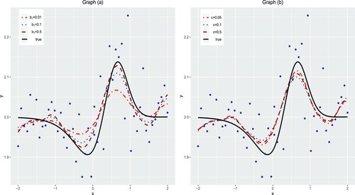
Table 1. ISEs for Gamma prior on δ and scaled Pareto prior on η.

	($a_1,b_1$)	(1,0.01)	(1,0.1)	(1,0.5)
Gamma($a_1,b_1)$	ISE	4.204$\times {10}^3$	2.189$\times {10}^3$	1.875$\times {10}^3$
Scaled Pareto$\left(c\right)$	c	0.05	0.1	0.5
	ISE	1.989$\times {10}^3$	2.142$\times {10}^3$	2.453$\times {10}^3$

4.2. Comparsion studies

Our comparison studies are conducted from two perspectives. For one thing, we evaluate the performance of our method by comparing with other four popular competing methods. For another, we investigate how the proposed method works when there are unobserved knots. We generate the data by, (27) $y_i=f\left(x_i\right)+a_p+{ϵ}_i,i=1,\dots ,n,$(27) where $f(\cdot )$ is a prespecified function and $a_p$ is the tuning number to ensure the pth quantile zero. We consider the following three distributions for the error term:

• Normal distribution, N$(0,{0.1}^2)$;

• ALD$(0,0.05,p)$, where p is the chosen quantile;

• Cauchy distribution with the location parameter 0 and the scale parameter 0.013, C$(0,0.013)$.

Given a quantile p and an error distribution above, we simulate 200 datasets. Within each dataset, we split it into one training dataset and one validation dataset. For the training dataset, we equally divide (0,1) into 20 spaces and simulate 5 observations at each knot. For the validation dataset, we equally divide (0,1) into 30 spaces and generate one observation at each knot. The validation dataset is employed to obtain the optimal regularisation parameter. We compare the different procedures by median of integrated absolute error (MIAE) and median of integrated square error (MISE), $\begin{array}{rl}\mathrm{M}\mathrm{I}\mathrm{A}\mathrm{E}& =\mathrm{m}\mathrm{e}\mathrm{d}\mathrm{i}\mathrm{a}\mathrm{n}\left({\int }_0^1\left|\hat{f}\left(x\right)f\left(x\right)\right|\mathrm{d}x\right),\\ \mathrm{M}\mathrm{I}\mathrm{S}\mathrm{E}& =\mathrm{m}\mathrm{e}\mathrm{d}\mathrm{i}\mathrm{a}\mathrm{n}\left({\int }_0^1{\left(\hat{f}\left(x\right)f\left(x\right)\right)}^2\mathrm{d}x\right),\end{array}$where median is taken over 200 simulation studies.

4.2.1. Comparison with candidate approaches

The Monte Carlo method is used to compare our method with other approaches including,

1. New Bayesian quantile smoothing spline (NBQSS);

2. Original Bayesian quantile smoothing spline (OBQSS) (Thompson et al., 2010);

3. Quantile smoothing spline (QSS) (Koenker et al., 1994);

4. Bayesian smoothing spline (BSS) (Tong et al., 2018);

5. Smoothing spline (SS) (Wahba, 1990).

We generate the data by (27(27) $y_i=f\left(x_i\right)+a_p+{ϵ}_i,i=1,\dots ,n,$(27) ) with the following two underlying curves (28) $\begin{array}{rl}\text{Curve I }:f\left(x\right)& =2+0.25\sin \left(0.25\text{π}x\right)\\ & +0.25\ln \left(x\right),0<x<1,\end{array}$(28) (29) $\begin{array}{rl}\text{Curve II}:f\left(x\right)& =2+0.2\sin \left(5\text{π}x\right)\\ & +0.25\ln \left(x\right),0<x<1.\end{array}$(29) The underlying Curve I is monotone and Curve II is a little bit twisted. For the smoothing parameter η in NBQSS, we adopt the scaled Pareto prior (20(20) $h\left(\eta \right)\propto \frac{c}{(c+\eta {)}^2},\eta >0,c>0.$(20) ) and the hyperparameter is chosen by GACV. For the smoothing parameter η in OBQSS, a Gamma$(\alpha ,\text{β})$ prior is utilised and its hyperparamters are selected in accordance with Thompson et al. (2010)'s suggestion. Specifically, $\text{β}=0.1/\mathrm{G}\mathrm{C}\mathrm{V}$(mean spline) and $\alpha =\mathrm{G}\mathrm{C}\mathrm{V}$(mean spline)$/\text{β}$, where GCV(mean spline) is the value of η chosen by the generalised cross-validation (Craven & Wahba, 1978). The numerical results for Curves I and II are listed in Tables 2 and 3, respectively.

Table 2. MIAEs and MISEs for Curve I with p = 0.1, 0.3 and 0.5.

		Error Distribution
		Normal		ALD		Cauchy
	Method	MIAE	MISE	MIAE	MISE	MIAE	MISE
p = 0.1	NBQSS	4.105$\times {10}^2$	2.607$\times {10}^3$	4.305$\times {10}^2$	3.495$\times {10}^3$	2.818$\times {10}^2$	1.355$\times {10}^3$
	OBQSS	1.796$\times {10}^1$	3.879$\times {10}^2$	1.328$\times {10}^1$	2.165$\times {10}^2$	2.403$\times {10}^1$	6.761$\times {10}^2$
	QSS	4.286$\times {10}^2$	2.998$\times {10}^3$	6.034$\times {10}^2$	5.916$\times {10}^3$	2.926$\times {10}^2$	1.383$\times {10}^3$
	BSS	2.774$\times {10}^2$	1.297$\times {10}^3$	9.654$\times {10}^2$	1.336$\times {10}^2$	3.512$\times {10}^2$	3.241$\times {10}^3$
	SS	2.557$\times {10}^2$	1.165$\times {10}^3$	1.038$\times {10}^1$	1.544$\times {10}^2$	4.543$\times {10}^2$	6.357$\times {10}^3$
p = 0.3	NBQSS	2.774$\times {10}^2$	1.476$\times {10}^3$	2.857$\times {10}^2$	1.609$\times {10}^3$	1.481$\times {10}^2$	8.329$\times {10}^4$
	OBQSS	5.697$\times {10}^2$	5.359$\times {10}^3$	5.622$\times {10}^2$	5.174$\times {10}^3$	6.593$\times {10}^2$	6.161$\times {10}^3$
	QSS	3.291$\times {10}^2$	1.733$\times {10}^3$	3.614$\times {10}^2$	2.309$\times {10}^3$	1.366$\times {10}^2$	5.372$\times {10}^4$
	BSS	2.417$\times {10}^2$	1.081$\times {10}^3$	4.143$\times {10}^2$	2.601$\times {10}^3$	3.239$\times {10}^2$	2.392$\times {10}^3$
	SS	2.522$\times {10}^2$	1.189$\times {10}^3$	3.981$\times {10}^2$	2.551$\times {10}^3$	3.231$\times {10}^2$	2.427$\times {10}^3$
p = 0.5	NBQSS	2.692$\times {10}^2$	1.152$\times {10}^3$	2.645$\times {10}^2$	1.284$\times {10}^3$	9.743$\times {10}^3$	3.461$\times {10}^4$
	OBQSS	4.373$\times {10}^2$	5.081$\times {10}^3$	4.296$\times {10}^2$	4.964$\times {10}^3$	3.718$\times {10}^2$	4.819$\times {10}^3$
	QSS	3.386$\times {10}^2$	1.906$\times {10}^3$	2.692$\times {10}^2$	1.308$\times {10}^3$	9.957$\times {10}^3$	3.538$\times {10}^4$
	BSS	2.667$\times {10}^2$	1.196$\times {10}^3$	3.318$\times {10}^2$	1.732$\times {10}^3$	2.677$\times {10}^2$	1.511$\times {10}^3$
	SS	2.559$\times {10}^2$	1.105$\times {10}^3$	3.341$\times {10}^2$	1.711$\times {10}^3$	2.756$\times {10}^2$	1.634$\times {10}^3$

Note: The bold numbers correspond to the smallest MIAE and MISE in each comparison.

Table 3. MIAEs and MISEs for Curve II with p = 0.1, 0.3 and 0.5.

		Error Distribution
		Normal		ALD		Cauchy
	Method	MIAE	MISE	MIAE	MISE	MIAE	MISE
p = 0.1	NBQSS	4.666$\times {10}^2$	3.269$\times {10}^3$	6.745$\times {10}^2$	6.844$\times {10}^3$	3.122$\times {10}^2$	2.118$\times {10}^3$
	OBQSS	2.351$\times {10}^1$	7.551$\times {10}^2$	1.764$\times {10}^1$	4.558$\times {10}^2$	3.017$\times {10}^1$	1.154$\times {10}^1$
	QSS	4.669$\times {10}^2$	3.282$\times {10}^3$	6.337$\times {10}^2$	6.351$\times {10}^3$	3.583$\times {10}^2$	2.379$\times {10}^3$
	BSS	2.832$\times {10}^2$	1.232$\times {10}^3$	1.144$\times {10}^1$	1.836$\times {10}^2$	5.098$\times {10}^2$	7.049$\times {10}^3$
	SS	3.051$\times {10}^2$	1.625$\times {10}^3$	1.105$\times {10}^1$	1.629$\times {10}^2$	5.198$\times {10}^2$	7.999$\times {10}^3$
p = 0.3	NBQSS	3.133$\times {10}^2$	1.501$\times {10}^3$	3.437$\times {10}^2$	1.951$\times {10}^3$	1.461$\times {10}^2$	5.264$\times {10}^4$
	OBQSS	1.309$\times {10}^1$	2.448$\times {10}^2$	1.261$\times {10}^1$	2.241$\times {10}^2$	1.444$\times {10}^1$	3.087$\times {10}^2$
	QSS	3.583$\times {10}^2$	1.984$\times {10}^3$	4.096$\times {10}^2$	2.555$\times {10}^3$	1.622$\times {10}^2$	6.108$\times {10}^4$
	BSS	2.761$\times {10}^2$	1.133$\times {10}^3$	4.799$\times {10}^2$	3.451$\times {10}^3$	3.353$\times {10}^2$	2.452$\times {10}^3$
	SS	2.925$\times {10}^2$	1.436$\times {10}^3$	4.889$\times {10}^2$	3.079$\times {10}^3$	3.721$\times {10}^2$	2.281$\times {10}^3$
p = 0.5	NBQSS	3.322$\times {10}^2$	1.775$\times {10}^3$	3.131$\times {10}^2$	1.588$\times {10}^3$	1.041$\times {10}^2$	2.712$\times {10}^4$
	OBQSS	1.169$\times {10}^1$	1.891$\times {10}^2$	1.175$\times {10}^1$	1.908$\times {10}^2$	1.165$\times {10}^1$	1.871$\times {10}^2$
	QSS	3.768$\times {10}^2$	2.364$\times {10}^3$	3.814$\times {10}^2$	2.369$\times {10}^3$	1.539$\times {10}^2$	5.329$\times {10}^4$
	BSS	2.795$\times {10}^2$	1.313$\times {10}^3$	3.587$\times {10}^2$	2.212$\times {10}^3$	3.189$\times {10}^2$	1.971$\times {10}^3$
	SS	3.006$\times {10}^2$	1.589$\times {10}^3$	3.612$\times {10}^2$	2.028$\times {10}^3$	3.847$\times {10}^2$	2.329$\times {10}^3$

Note: The bold numbers correspond to the smallest MIAE and MISE in each comparison.

From Tables 2 and 3, NBQSS uniformly outperforms OBQSS, which indicates our method serves as an efficient improvement over the original method. Among three quantile methods (NBQSS, OBQSS and QSS), NBQSS performs best with the lowest MIAE and MISE in 8 out of 9 comparisons. However, when the error is the normal distribution, two mean regression methods (BSS and SS) perform better than three quantile regression methods with lower MIAE and MISE. In contrast, when the error is the ALD or the Cauchy, two quantile approaches (NBQSS and QSS) have better performances for all the selected quantiles. In addition, OBQSS has the worst performance among the five candidate methods no matter which quantiles or random errors are used. Also, OBQSS tends to perform worse as p is away from 0.5, which echoes the findings in Santos and Bolfarine (2016). Although a similar trend appears in all quantile methods, compared with other candidate models, our method still shows considerable advantages.

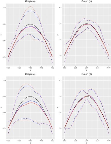
We also demonstrate the behaviours of fitted curves for Curves I and II with ALD error and p = 0.3. In the 200 simulation studies, we can obtain the fitted value for any point $x\in (0,1)$. We treated the median of the 200 simulation studies at the point x as the estimation and draw the fitted curves in Figures 2 and 3. We also plot the pointwise empirical 2.5% and 97.5% quantiles of the 200 estimates to display the variability in estimation.

Figure 2. The curves are fitted for Curve I under p = 0.3 and ALD error. Graph (a) NBQSS method; Graph (b) OBQSS method; Graph (c) QSS method; Graph (d) BSS method; Graph (e) SS method. The solid lines are  the true curve and the fitted curve. Two dashed lines are 2.5% and 97.5% pointwise empirical quantiles.

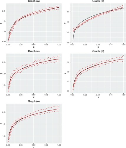
Figure 3. The curves are fitted for Curve II under p = 0.3 and ALD error. Graph (a) NBQSS method; Graph (b) OBQSS method; Graph (c) QSS method; Graph (d) BSS method; Graph (e) SS method. The solid lines are the true curve and the fitted curve. Two dashed lines are 2.5% and 97.5% pointwise empirical quantiles.

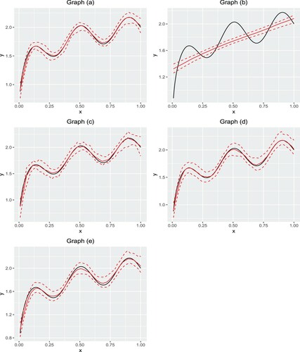
From Figures 2 and 3, we may find that OBQSS tends to give a relatively flat curve, which fails to capture the true trend in the curve, especially when the curve is twisted. Based on our experience, in this case, OBQSS chooses large values for η, which results in a flat fitted curve. For example, for Curve I with p = 0.3 and ALD distributed random errors, the posterior median of η in NBQSS is 0.004 while in OBQSS is 1.135. This phenomenon requires further investigation.

4.2.2. Comparison of NBQSS with and without unobserved knots

We investigate how NBQSS performs with unobserved knots. We generate the data by (27(27) $y_i=f\left(x_i\right)+a_p+{ϵ}_i,i=1,\dots ,n,$(27) ) with the underlying curve (30) $f\left(x\right)=0.8\sin \left(\text{π}x\right),0<x<1.$(30) We equally divide (0,1) into 20 spaces and regard it as the complete knots. Two representative unobserved knots mechanisms are considered,

• Mechanism I:  α% of the complete knots are unobserved in the middle.

• Mechanism II:  two knots around 0.5 have observations and $\left(\alpha /2\right)$% of the complete knots are unobserved in each of two intervals, (0,0.47) and (0.52,1).

We take $\alpha \mathrm{\%}=$ 30%, 50% and 70% to represent low, medium and high unobserved proportion. For each observed knot, we randomly generate 5 observations. We illustrate the above two mechanisms in Figure 4. We implement the regular NBQSS (without unobserved knots) and NBQSS with unobserved knots (we refer it to NBQSSK, ‘K’ is for knot). For Mechanism I, we add 6 uniformly distributed knots in total for the interval without knots. For Mechanism II, we add 3 uniformly distributed knots in each of two intervals without knots, hence 6 unobserved knots in total. We consider p = 0.1, 0.5 and 0.9. MIAEs and MISEs are recorded in Tables 4 and 5.

Figure 4. One illustration for Mechanisms I and II. Graphs (a)–(c) correspond to Mechanism I with $\alpha \mathrm{\%}=30\mathrm{\%},50\mathrm{\%}$ and 70%. Graphs (d) and (e) correspond to Mechanism II with $\alpha \mathrm{\%}=$30%, 50% and 70%.

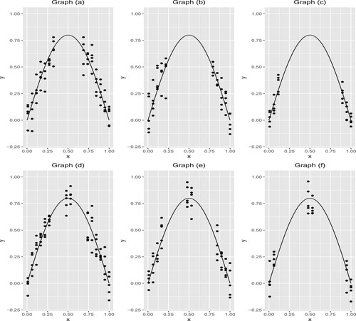
Table 4. MIAEs and MISEs for Mechanism I with quantiles p = 0.1, 0.5, 0.9 and unobserved proportions $\alpha \mathrm{\%}=30\mathrm{\%},50\mathrm{\%},70\mathrm{\%}$.

			Error Distribution
			Normal		ALD		Cauchy
		Method	MIAE	MISE	MIAE	MISE	MIAE	MISE
30%	p = 0.1	NBQSS	3.985$\times {10}^2$	2.288$\times {10}^3$	4.422$\times {10}^2$	2.921$\times {10}^3$	4.147$\times {10}^2$	3.956$\times {10}^3$
		NBQSSK	3.786$\times {10}^2$	2.111$\times {10}^3$	4.463$\times {10}^2$	3.011$\times {10}^3$	3.865$\times {10}^2$	3.180$\times {10}^3$
	p = 0.5	NBQSS	2.759$\times {10}^2$	1.040$\times {10}^3$	2.733$\times {10}^2$	1.157$\times {10}^3$	7.713$\times {10}^3$	1.007$\times {10}^4$
		NBQSSK	2.688$\times {10}^2$	9.876$\times {10}^4$	2.561$\times {10}^2$	1.046$\times {10}^3$	7.566$\times {10}^3$	9.603$\times {10}^5$
	p = 0.9	NBQSS	4.686$\times {10}^2$	3.339$\times {10}^3$	4.647$\times {10}^2$	3.809$\times {10}^3$	4.007$\times {10}^2$	3.478$\times {10}^3$
		NBQSSK	4.482$\times {10}^2$	2.856$\times {10}^3$	4.705$\times {10}^2$	3.642$\times {10}^3$	4.314$\times {10}^2$	3.744$\times {10}^3$
50%	p = 0.1	NBQSS	6.968$\times {10}^2$	6.790$\times {10}^3$	7.258$\times {10}^2$	7.435$\times {10}^3$	5.464$\times {10}^2$	5.551$\times {10}^3$
		NBQSSK	6.336$\times {10}^2$	5.231$\times {10}^3$	7.223$\times {10}^2$	7.543$\times {10}^3$	4.878$\times {10}^2$	4.746$\times {10}^3$
	p = 0.5	NBQSS	4.344$\times {10}^2$	2.741$\times {10}^3$	4.526$\times {10}^2$	2.744$\times {10}^3$	1.530$\times {10}^2$	3.619$\times {10}^4$
		NBQSSK	4.235$\times {10}^2$	2.505$\times {10}^3$	4.308$\times {10}^2$	2.532$\times {10}^3$	1.494$\times {10}^2$	3.767$\times {10}^4$
	p = 0.9	NBQSS	7.627$\times {10}^2$	8.700$\times {10}^3$	6.108$\times {10}^2$	5.865$\times {10}^3$	7.548$\times {10}^2$	9.166$\times {10}^3$
		NBQSSK	6.983$\times {10}^2$	7.093$\times {10}^3$	5.440$\times {10}^2$	4.738$\times {10}^3$	6.487$\times {10}^2$	6.920$\times {10}^3$
70%	p = 0.1	NBQSS	1.134$\times {10}^1$	1.698$\times {10}^2$	2.174$\times {10}^1$	2.784$\times {10}^2$	1.487$\times {10}^1$	3.685$\times {10}^2$
		NBQSSK	1.008$\times {10}^1$	1.345$\times {10}^2$	1.582$\times {10}^1$	2.043$\times {10}^2$	1.222$\times {10}^1$	2.741$\times {10}^2$
	p = 0.5	NBQSS	8.685$\times {10}^2$	9.997$\times {10}^3$	7.782$\times {10}^2$	8.777$\times {10}^3$	4.316$\times {10}^2$	3.075$\times {10}^3$
		NBQSSK	8.377$\times {10}^2$	9.539$\times {10}^3$	6.850$\times {10}^2$	6.965$\times {10}^3$	4.349$\times {10}^2$	3.098$\times {10}^3$
	p = 0.9	NBQSS	1.156$\times {10}^1$	2.053$\times {10}^2$	1.593$\times {10}^1$	3.805$\times {10}^2$	1.592$\times {10}^1$	3.652$\times {10}^2$
		NBQSSK	1.117$\times {10}^1$	1.772$\times {10}^2$	1.467$\times {10}^1$	2.975$\times {10}^2$	1.416$\times {10}^1$	2.859$\times {10}^2$

Notes: The number of observations varies across different observed knots. The bold numbers correspond to the smallest MIAE and MISE in each comparison.

Table 5. MIAEs and MISEs for Mechanism II with quantiles p = 0.1, 0.5, 0.9 and unobserved proportions $\alpha \mathrm{\%}=30\mathrm{\%},50\mathrm{\%},70\mathrm{\%}$.

			Error Distribution
			Normal		ALD		Cauchy
		Method	MIAE	MISE	MIAE	MISE	MIAE	MISE
30%	p = 0.1	NBQSS	4.196$\times {10}^2$	2.607$\times {10}^3$	4.215$\times {10}^2$	2.575$\times {10}^3$	4.405$\times {10}^2$	3.849$\times {10}^3$
		NBQSSK	4.017$\times {10}^2$	2.299$\times {10}^3$	4.271$\times {10}^2$	2.595$\times {10}^3$	4.187$\times {10}^2$	3.336$\times {10}^3$
	p = 0.5	NBQSS	2.565$\times {10}^2$	9.338$\times {10}^4$	2.673$\times {10}^2$	1.040$\times {10}^3$	7.159$\times {10}^3$	8.339$\times {10}^5$
		NBQSSK	2.458$\times {10}^2$	9.094$\times {10}^4$	2.631$\times {10}^2$	1.037$\times {10}^3$	7.173$\times {10}^3$	7.987$\times {10}^5$
	p = 0.9	NBQSS	3.924$\times {10}^2$	2.235$\times {10}^3$	4.787$\times {10}^2$	3.176$\times {10}^3$	5.495$\times {10}^2$	5.160$\times {10}^3$
		NBQSSK	3.947$\times {10}^2$	2.166$\times {10}^3$	4.715$\times {10}^2$	3.098$\times {10}^3$	5.086$\times {10}^2$	4.271$\times {10}^3$
50%	p = 0.1	NBQSS	4.884$\times {10}^2$	3.485$\times {10}^3$	5.422$\times {10}^2$	4.058$\times {10}^3$	5.614$\times {10}^2$	5.494$\times {10}^3$
		NBQSSK	4.666$\times {10}^2$	3.186$\times {10}^3$	5.318$\times {10}^2$	3.658$\times {10}^3$	5.090$\times {10}^2$	5.160$\times {10}^3$
	p = 0.5	NBQSS	3.215$\times {10}^2$	1.548$\times {10}^3$	3.567$\times {10}^2$	1.912$\times {10}^3$	9.201$\times {10}^3$	1.250$\times {10}^4$
		NBQSSK	3.112$\times {10}^2$	1.449$\times {10}^3$	3.532$\times {10}^2$	1.819$\times {10}^3$	8.622$\times {10}^3$	1.147$\times {10}^4$
	p = 0.9	NBQSS	5.653$\times {10}^2$	4.493$\times {10}^3$	5.798$\times {10}^2$	4.931$\times {10}^3$	6.294$\times {10}^2$	7.644$\times {10}^3$
		NBQSSK	5.146$\times {10}^2$	3.487$\times {10}^3$	5.366$\times {10}^2$	4.437$\times {10}^3$	6.565$\times {10}^2$	8.191$\times {10}^3$
70%	p = 0.1	NBQSS	7.133$\times {10}^2$	7.174$\times {10}^3$	3.479$\times {10}^2$	1.779$\times {10}^3$	8.868$\times {10}^2$	1.204$\times {10}^2$
		NBQSSK	6.598$\times {10}^2$	5.856$\times {10}^3$	3.173$\times {10}^2$	1.449$\times {10}^3$	8.655$\times {10}^2$	1.096$\times {10}^2$
	p = 0.5	NBQSS	5.498$\times {10}^2$	4.099$\times {10}^3$	1.731$\times {10}^2$	4.062$\times {10}^4$	1.840$\times {10}^2$	5.022$\times {10}^4$
		NBQSSK	5.246$\times {10}^2$	3.654$\times {10}^3$	1.655$\times {10}^2$	3.733$\times {10}^4$	1.841$\times {10}^2$	5.010$\times {10}^4$
	p = 0.9	NBQSS	9.509$\times {10}^2$	1.329$\times {10}^2$	3.730$\times {10}^2$	2.211$\times {10}^3$	7.432$\times {10}^2$	7.884$\times {10}^3$
		NBQSSK	9.040$\times {10}^2$	1.182$\times {10}^2$	3.373$\times {10}^2$	1.787$\times {10}^3$	7.076$\times {10}^2$	6.899$\times {10}^3$

Notes: The number of observations varies across different observed knots. The bold numbers correspond to the smallest MIAE and MISE in each comparison.

In Tables 4 and 5, we may find two similarities for NBQSS and NBQSSK. Firstly, as α increases, the prediction errors increase for two methods. Secondly, both methods perform the best for p = 0.5 compared with other selected quantiles. In addition, based on Tables 4 and 5, for brevity, Table 6 summarises the percentage where NBQSSK outperforms NBQSS in each cell across different combinations of unobserved proportions and error distributions. From Table 6, we may find that NBQSSK defeats NBQSS in all the scenarios, especially for a large α, which substantiates that NBQSSK can provide the better prediction compared with regular NBQSS.

Table 6. Summary of cases where NBQSSK outperforms NBQSS.

	Error Distribution
Mechanism I	Normal	ALD	Cauchy
30%	100%	50%	66.7%
50%	100%	83.3%	83.3%
70%	100%	100%	66.7%
	Error Distribution
Mechanism II	Normal	ALD	Cauchy
30%	83.3%	66.7%	83.3%
50%	100%	100%	67.6%
70%	100%	100%	83.3%

Note: Each cell is the proportion of the winning cases of NBQSSK out of six comparisons.

Furthermore, to offer a more intuitive comparison of NBQSS and NBQSSK, we present the fitted curves and their empirical 95% credible intervals with quantile p = 0.1, ALD random error for Mechanisms I and II setting the unobserved proportion $\alpha \mathrm{\%}$=50% and 70%. From Figure 5, we have several main findings. Firstly, NBQSSK performs similarly compared with NBQSS in the interval with observed knots. Secondly, two methods provide wider empirical credible intervals for Mechanism I than Mechanism II. It implies that the uncertainty surges when there is no guided information in the middle. Thirdly, for Mechanism I, the empirical 95% credible intervals of the NBQSSK are shorter than the NBQSS, especially in the middle interval. It reveals that NBQSSK can provide a more efficient uncertainty evaluation for the unobserved knots. However, the advantage of NBQSSK is less obvious for Mechanism II. Besides, for Mechanism I, NBQSSK is more advantageous than NBQSS when the unobserved proportion $\alpha \mathrm{\%}=70\mathrm{\%}$ compared with $\alpha \mathrm{\%}=50\mathrm{\%}$, which echoes our findings in Tables 4 and 5. At last, for Mechanism I or II, compared with $\alpha \mathrm{\%}=50\mathrm{\%}$, $\alpha \mathrm{\%}=70\mathrm{\%}$ has wider empirical 95% credible interval widths.

Figure 5. The solid lines are the true curve and fitted curves. The curves are fitted with p = 0.1, ALD random error. Dashed lines are empirical 95% credible interval corresponding to NBQSSK and dotted lines are empirical 95% credible interval corresponding to NBQSS. Graph (a): Mechanism I, $\alpha \mathrm{\%}=50\mathrm{\%}$; Graph (b): corresponds to Mechanism II, $\alpha \mathrm{\%}=50\mathrm{\%}$; Graph (c): Mechanism I, $\alpha \mathrm{\%}=70\mathrm{\%}$; Graph (d): Mechanism II, $\alpha \mathrm{\%}=70\mathrm{\%}$.

Remark 4.1

Notice that the above simulation studies are based on 5 observations at each observed knot. In fact, we have also conducted simulation studies with unequal number of observations at each observed knot. The main findings are similar to Tables 4 and 5. This implies that the relative performance of NBQSSK and NBQSS is irrespective of the number of observations at each observed knot.

4.3. Real dataset

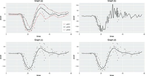
4.3.1. Motorcycle dataset

We analysed the well-known data utilised by Silverman (1985) to demonstrate nonparametric regression curve fitting. It has been frequently used to motivate and demonstrate the spline-based methodology, since the underlying curve makes polynomial modelling inappropriate. There are 113 observations in the data including accelerometer readings taken through time in an experiment on the efficacy of crash helmet. For NBQSS, we fit the quantile curves with p = 0.1, 0.5 and 0.9. To assess their performances, we fit the median curve with OBQSS and the mean curves with BSS and SS. Figure 6 shows the fitted curves of these methods. In Graph (a), with p = 0.5, NBQSS captures the general trend. With more quantiles, NBQSS offers an overview of the distribution. Interestingly, in Graph (b), the curve fitted using OBQSS is jittering very much, which tends to overfit. Similar results can be found in OBQSS when p = 0.1 and 0.9 (not shown here). Compared with NBQSS, the estimation of smoothing parameter is $8.167\times {10}^6$ while is 0.068 in NBQSS. Compared with two mean curve fitting methods, we record the median of absolute deviation (MAD) defined as (31) $\mathrm{M}\mathrm{A}\mathrm{D}=\mathrm{m}\mathrm{e}\mathrm{d}\mathrm{i}\mathrm{a}\mathrm{n}\left(\left|y_i{\hat{y}}_i\right|\right),i=1,\dots ,113.$(31) for each method. The MAD for NBQSS with p = 0.5, BSS and SS is 8.755, 12.979 and 13.02781, respectively. It indicates that the median curve fitted by NBQSS are relatively robust to the points with big deviation compared with mean curve fitting methods.

Figure 6. Graph (a): NBQSS method with p = 0.1, 0.5 and 0.9; Graph (b): OBQSS method with p = 0.5; Graph (c): BSS method; Graph (d): SS method.

4.3.2. China bond medium term note

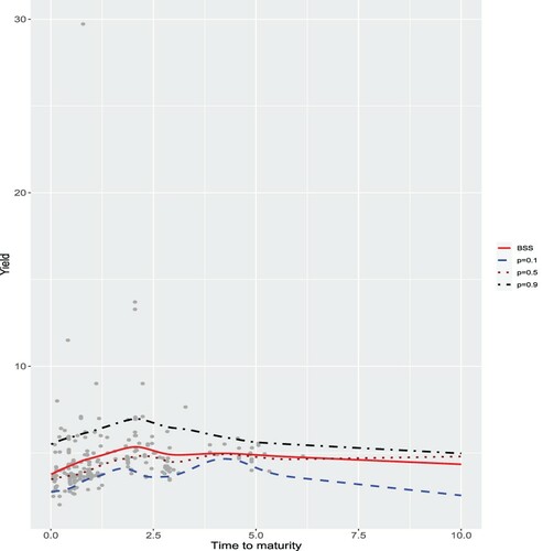
The term structure of interest rates is the series of interest rates ordered by time to maturity at a given time. It is a fundamental concept in economic and financial theory such as fixed-income securities analysis, pricing derivatives, performing hedging operations, etc. The ‘term structure of interest rates’ is also known as a yield curve. In financial markets, there are a limited number of bonds traded, so an interpolation method is necessary to estimate the yield cuvre across the whole maturity spectrum. Tong et al. (2018) employed the BSS to fit China bond yield curve and the simulation studies show that BSS outperforms the traditional yield curve fitting methods such as Nelson-Siegel model (Nelson & Siegel, 1987) and Svensson extension model (Svensson, 1994). However, when fitting the yield curve for China Bond Medium Term Note (CBMTN), which is one kind of bond issued by corporation or company to collect the capital, there always exist some underlying outliers disturbing the signals. In comparison to BSS, we employ NBQSS to obtain the quantile curves for CBMTN. The data set is downloaded from Wind (https://www.wind.com.cn/). This analysis focuses on the yield curve of CBMTN rating ‘CAAA’ on 25 September 2018, which is the highest rating of this bond and associated with lowest yield but lowest risk. There are 282 transaction data in CBMTN and there exist some obvious abnormal transactions in the data. Figure 7 shows us the NBQSS curves for p = 0.1, 0.5 and 0.9 along with BSS curve. The transaction data are marked as grey points. We may find that the BSS curve is overall lifted up by the outliers compared with the NBQSS using p = 0.5, especially when the time to maturity belongs to [0,5]. The results imply that the quantile curves using NBQSS are robust to the possible outliers while BSS is not. In addition, we record MAD for NBQSS with p = 0.5 and BSS. The MAD for NBQSS with p = 0.5 is 0.451 and for BSS is 0.79, which indicates that NBQSS provides more accurate estimation compared with BSS.

Figure 7. BSS curve (solid) and NBQSS with $p=$0.1 (dashed), 0.5 (dotted) and 0.9 (dotted-dash) curves on 25 September 2018.

5. Comments

In this paper, we numerically demonstrate the issue associated with a fixed σ in OBQSS. To serve as a solution, we systematically investigate NBQSS with a random scale parameter. We establish conditions for the posterior propriety of the NBQSS under two common prior options, conjugate priors for $(\sigma ,\delta )$ and one general prior $1/{\sigma }^{a+1}h\left(\eta \right)$ on $(\sigma ,\eta )$. These conditions are easy for practitioners to verify, hence serve as a guide to specify priors. We recommend imposing the prior on $(\sigma ,\eta )$ rather than $(\sigma ,\delta )$ to an ensured proper joint posterior and a relatively robust hyperparameter specification. In practice, it is often for researchers to face unobserved knots when dealing with curve fitting. Therefore, we extend our theoretical results to NBQSS with unobserved knots. Finally, our simulation studies imply that our NBQSS performs the best in candidate quantile methods and NBQSS with unobserved knots perform better than regular NBQSS for most of cases. As with any simulation study, these cannot cover all possibilities, but we believe that they are sufficiently wide ranging to provide useful insights into the comparative performance of the different procedures.

Several unsolved issues in our work still worth investigating. For example, as shown in the simulation studies, all quantile methods perform relatively worse near the boundary, such as p = 0.1, and more work is encouraged to improve their boundary behaviours under the Bayesian framework. Also, when there are unobserved knots, how to choose the positions of added knots and how to decide the number of added knots to obtain better fitted curves are of interest in NBQSS. Furthermore, we do not consider the crossing problem for different quantiles in this article. Without special restriction, quantile regression functions estimated at different orders can cross each other, which disobeys the rule of the probability. Therefore, another concern is to develop the theoretical results for the non-crossing Bayesian regularised regression quantile (Liu & Wu, 2011).

Acknowledgements

The authors sincerely thank two anonymous reviewers for the thoughtful and constructive suggestions they provided that led to considerable improvements in the presentation of our work.

Disclosure statement

No potential conflict of interest was reported by the authors.

Additional information

Funding

The project was supported by the National Natural Science Foundation of China [Grant Number 11671146].

Notes on contributors

Zhongheng Cai

Zhongheng Cai is a PhD candidate in the school of statistics, East China Normal University, Shanghai, China. His research interests include Bayesian statistics.

Dongchu Sun

Dr. Dongchu Sun received his PhD. in 1991 from Department of Statistics, Purdue University, under the guidance of Professor James O. Berger.

Appendices

Appendix 1. Proof of Theorem 2.1

Proof.

With the likelihood (14(14) $p(\mathit{y}|\mathit{z},p,\sigma )\propto {\sigma }^N\exp \left\{\sigma {\rho }_p(\mathit{y}\mathit{C}\mathit{z})\right\},$(14) ) and priors (15(15) $\pi \left(\mathit{z}|\delta \right)\propto \frac{|\mathit{A}{|}_{+}^{1/2}}{{\delta }^{(n2)/2}}\exp \left(\frac{1}{2\delta }{\mathit{z}}^{\mathrm{\prime }}\mathit{A}\mathit{z}\right),$(15) ), (16(16) $\pi (\sigma ,\delta )\propto {\sigma }^{a_{0}1}\exp (b_0\sigma )\frac{1}{{\delta }^{a_1+1}}\exp \left(\frac{b_1}{\delta }\right).$(16) ), the posterior of $(\mathit{z},\sigma ,\delta |\mathit{y})$ is proportional to (A1) $\begin{array}{rl}& {\sigma }^{N+a_{0}1}\exp \left(\sigma {\rho }_p(\mathit{y}\mathit{C}\mathit{z})\frac{1}{2\delta }{\mathit{z}}^{\mathrm{\prime }}\mathit{A}\mathit{z}\right)\\ & \times \exp (b_0\sigma )\frac{1}{{\delta }^{a_1+\frac{n2}{2}+1}}\exp \left(\frac{b_1}{\delta }\right).\end{array}$(A1) Integrate σ, (A1(A1) $\begin{array}{rl}& {\sigma }^{N+a_{0}1}\exp \left(\sigma {\rho }_p(\mathit{y}\mathit{C}\mathit{z})\frac{1}{2\delta }{\mathit{z}}^{\mathrm{\prime }}\mathit{A}\mathit{z}\right)\\ & \times \exp (b_0\sigma )\frac{1}{{\delta }^{a_1+\frac{n2}{2}+1}}\exp \left(\frac{b_1}{\delta }\right).\end{array}$(A1) ) is proportional to (A2) $\frac{1}{{\left[{\rho }_p\left(\mathit{y}\mathit{C}\mathit{z}\right)+b_0\right]}^{N+a_0}}\frac{1}{{\delta }^{\frac{n2}{2}+a_1+1}}\exp \left(\frac{1}{2\delta }{\mathit{z}}^{\mathrm{\prime }}\mathit{A}\mathit{z}\frac{b_1}{\delta }\right).$(A2) We only prove the sufficiency, the necessity can be proved in the similar way.

Since $min\{p,1p\}|\mathit{z}{|}_1\le {\rho }_p\left(\mathit{z}\right)\le max\{p,1p\}|\mathit{z}{|}_1,$ and $||\mathit{z}|{|}_2\le |\mathit{z}{|}_1\le \sqrt{n}||\mathit{z}|{|}_2,\mathrm{\forall }\mathit{z}\in {\mathbb{R}}^n,$ there exists a positive number $M_1$ such that (A3) ${\rho }_p(\mathit{y}\mathit{C}\mathit{z})+b_0\ge \sqrt{M_1(\mathit{y}\mathit{C}\mathit{z}{)}^{\mathrm{\prime }}(\mathit{y}\mathit{C}\mathit{z})}+b_0.$(A3) Moreover, there exist $M_2>0,$ such that (A4) $\left(\text{A}3\right)\ge M_2\sqrt{M_1(\mathit{y}\mathit{C}\mathit{z}{)}^{\mathrm{\prime }}(\mathit{y}\mathit{C}\mathit{z})+b_0}.$(A4) Hence, we just need to consider, (A5) $\begin{array}{rl}& \frac{1}{{\left[\sqrt{M_1(\mathit{y}\mathit{C}\mathit{z}{)}^{\mathrm{\prime }}(\mathit{y}\mathit{C}\mathit{z})+b_0}\right]}^{N+a_0}}\frac{1}{{\delta }^{\frac{n2}{2}+a_1+1}}\\ & \times \exp \left(\frac{1}{2\delta }{\mathit{z}}^{\mathrm{\prime }}\mathit{A}\mathit{z}\frac{b_1}{\delta }\right).\end{array}$(A5) We consider (A6) $\begin{array}{rl}& \frac{1}{{\sigma }_1^{\frac{N+a_0}{2}+1}}\frac{1}{{\delta }^{\frac{n2}{2}}}\\ & \times \exp \left(\frac{M_1}{{\sigma }_1}(\mathit{y}\mathit{C}\mathit{z}{)}^{\mathrm{\prime }}(\mathit{y}\mathit{C}\mathit{z})\frac{b_0}{{\sigma }_1}\frac{1}{2\delta }{\mathit{z}}^{\mathrm{\prime }}\mathit{A}\mathit{z}\right)\\ & \times \frac{1}{{\delta }^{a_1+1}}\exp \left(\frac{b_1}{\delta }\right),\end{array}$(A6) since the integration with respect to ${\sigma }_1$ is proportional to (A5(A5) $\begin{array}{rl}& \frac{1}{{\left[\sqrt{M_1(\mathit{y}\mathit{C}\mathit{z}{)}^{\mathrm{\prime }}(\mathit{y}\mathit{C}\mathit{z})+b_0}\right]}^{N+a_0}}\frac{1}{{\delta }^{\frac{n2}{2}+a_1+1}}\\ & \times \exp \left(\frac{1}{2\delta }{\mathit{z}}^{\mathrm{\prime }}\mathit{A}\mathit{z}\frac{b_1}{\delta }\right).\end{array}$(A5) ). Now, set ${\mathit{y}}_1=\sqrt{2M_1}\mathit{y},{\mathit{z}}_1=\sqrt{2M_1}\mathit{z},{\mathit{A}}_1=\frac{1}{2M_1}\mathit{A}$, (A6(A6) $\begin{array}{rl}& \frac{1}{{\sigma }_1^{\frac{N+a_0}{2}+1}}\frac{1}{{\delta }^{\frac{n2}{2}}}\\ & \times \exp \left(\frac{M_1}{{\sigma }_1}(\mathit{y}\mathit{C}\mathit{z}{)}^{\mathrm{\prime }}(\mathit{y}\mathit{C}\mathit{z})\frac{b_0}{{\sigma }_1}\frac{1}{2\delta }{\mathit{z}}^{\mathrm{\prime }}\mathit{A}\mathit{z}\right)\\ & \times \frac{1}{{\delta }^{a_1+1}}\exp \left(\frac{b_1}{\delta }\right),\end{array}$(A6) ) becomes $\begin{array}{rl}& \frac{1}{{\sigma }_1^{\frac{N+a_0}{2}+1}}\frac{1}{{\delta }^{\frac{n2}{2}}}\\ & \times \exp \left(\frac{1}{2{\sigma }_1}({\mathit{y}}_1\mathit{C}{\mathit{z}}_1{)}^{\mathrm{\prime }}({\mathit{y}}_1\mathit{C}{\mathit{z}}_1)\frac{b_0}{{\sigma }_1}\frac{1}{2\delta }{\mathit{z}}_1^{\mathrm{\prime }}{\mathit{A}}_1{\mathit{z}}_1\right)\\ & \times \frac{1}{{\delta }^{a_1+1}}\exp \left(\frac{b_1}{\delta }\right),\end{array}$which agrees with the case for normal error in Speckman and Sun (2003), the results follow.

Appendix 2. Proof of Theorem 2.2

For $\left(a\right)$, the following lemma is needed,

Lemma A.1

Assume $Z\sim N(0,{\sigma }^2)$, for any $t>0,\mu \in \mathbb{R}$,

1. (A7) $\begin{array}{rl}& 2\sqrt{\frac{2}{\text{π}}}\frac{\sigma t}{1+{\sigma }^2{t}^2}\exp \left(\frac{{\mu }^2}{2{\sigma }^2}\right)\\ & \le E\left(\exp \left(t|Z\mu |\right)\right)\\ & \le min\left\{1,\sqrt{\frac{2}{e\text{π}}}\frac{1}{t|\mu |}\right\}\le \sqrt{\frac{2}{1+\frac{\text{π}e}{2}{\mu }^2{t}^2}},\end{array}$(A7)

2. (A8) $\begin{array}{rl}& E\left(\exp \left(t|Z\mu |\right)\right)\\ & \le \sqrt{\frac{2}{\text{π}}}\frac{1}{\sigma t}\exp \left(\frac{{\mu }^2}{4{\sigma }^2}\right)+\exp \left(\frac{\mu t}{\sqrt{2}}\right).\end{array}$(A8)

Proof.

For (1), the third inequality is trivial, we focus on the other two inequalities. For the first one, we have, $\begin{array}{rl}& E\left(\exp \left(t|Z\mu |\right)\right)\\ & ={\int }_{\mathrm{\infty }}^{+\mathrm{\infty }}\frac{1}{\sigma \sqrt{2\text{π}}}\exp \left(t|z\mu |\frac{z^2}{2{\sigma }^2}\right)\mathrm{d}z\\ & ={\int }_{\mathrm{\infty }}^{+\mathrm{\infty }}\frac{1}{\sigma \sqrt{2\text{π}}}\exp \left(t\left|z\right|\frac{(z+\mu {)}^2}{2{\sigma }^2}\right)\mathrm{d}z\\ & =\exp \left(\frac{{\mu }^2}{2{\sigma }^2}\right){\int }_{\mathrm{\infty }}^{+\mathrm{\infty }}\frac{1}{\sigma \sqrt{2\text{π}}}\\ & \times \exp \left(t|z|\frac{z^2}{2\sigma }\frac{z\mu }{{\sigma }^2}\right)\mathrm{d}z\\ & =\exp \left(\frac{{\mu }^2}{2{\sigma }^2}\right){\int }_0^{+\mathrm{\infty }}\frac{1}{\sigma \sqrt{2\text{π}}}\exp \left(t|z|\frac{z^2}{2{\sigma }^2}\right)\\ & \times \left(\exp \left(\frac{z\mu }{{\sigma }^2}\right)+\exp \left(\frac{z\mu }{{\sigma }^2}\right)\right)\mathrm{d}z.\end{array}$By arithmetic-geometric mean inequality, $\exp \left(z\mu /{\sigma }^2\right)+\exp (z\mu /{\sigma }^2)\ge 2$. Hence, $E\left(\exp \left(t|Z\mu |\right)\right)\ge 2\exp \left(\frac{{\mu }^2}{2{\sigma }^2}\right)E\left(\exp \left(t|Z|\right)\right).$We can obtain $E\left(\exp \left(t|Z|\right)\right)=\sqrt{\frac{2}{\text{π}}}\frac{\left(1\mathrm{\Phi }\left(t\sigma \right)\right)}{\varphi \left(t\sigma \right)},$where Φ, ϕ are standard normal c.d.f and p.d.f respectively. By the inequality (Gordon, 1941) $\frac{t}{1+t^2}\le \frac{1\mathrm{\Phi }\left(t\right)}{\varphi \left(t\right)}\le \frac{1}{t},\mathrm{\forall }t>0,$the first inequality holds. For the second inequality, we need the hierarchical structure of the Laplace distribution. Andrews and Mallows (1974) proposed that (A9) $\begin{array}{rl}& \frac{t}{2}\exp \left(t|Z\mu |\right)\\ & ={\int }_0^{+\mathrm{\infty }}\frac{1}{\sqrt{2\text{π}}y}\exp \left(\frac{(Z\mu {)}^2}{2y^2}\right)t^{2}y\exp \left(\frac{y^2{t}^2}{2}\right)\mathrm{d}y.\end{array}$(A9) Hence, by Fubini's theorem, (A10) $\begin{array}{rl}& \frac{t}{2}E(\exp (t|Z\mu |\left)\right)\\ & ={\int }_0^{+\mathrm{\infty }}{\int }_{\mathrm{\infty }}^{+\mathrm{\infty }}\left\{\frac{1}{\sqrt{2\text{π}}\sigma }\frac{1}{\sqrt{2\text{π}}y}\right.\\ & \times \left.\exp \left(\frac{(z\mu {)}^2}{2y^2}\frac{z^2}{2{\sigma }^2}\right)\mathrm{d}z\right\}{t}^{2}y\exp \left(\frac{y^2{t}^2}{2}\right)\mathrm{d}y.\end{array}$(A10) Since $\mu |z,y\sim N(z,y^2)$, $z|{\sigma }^2\sim N(0,{\sigma }^2)$, we have the marginal distribution of $\mu |y,{\sigma }^2$ is $N(0,{\sigma }^2+y^2)$. The inner integral equals (A11) $I(\mu ,y)=\sqrt{\frac{1}{2\text{π}({\sigma }^2+y^2)}}\exp \left(\frac{{\mu }^2}{2{\sigma }^2+2y^2}\right).$(A11) Since the function $f\left(w\right)=1/w\exp ({\mu }^2/(2w\left)\right),w={\sigma }^2+y^2,$ is unimodal with the maximum value $|\mu {|}^1\exp (1/2),$ we have $I(\mu ,y)\le \frac{1}{\sqrt{2\text{π}\mathrm{e}}|\mu |}.$Hence, $E\left(\exp \left(t|Z\mu |\right)\right)\le \sqrt{\frac{2}{\text{π}\mathrm{e}}}\frac{1}{|\mu |t}.$Clearly, $E(\exp (t|x\mu |\left)\right)\le 1$, so the second inequality holds.

For (2), since (A12) $\begin{array}{rl}& \frac{t}{2}E(\exp (t|Z\mu |\left)\right)\\ & ={\int }_0^{+\mathrm{\infty }}\sqrt{\frac{1}{2\text{π}({\sigma }^2+y^2)}}{t}^{2}y\\ & \times \exp \left(\frac{{\mu }^2}{2{\sigma }^2+2y^2}\frac{y^2{t}^2}{2}\right)\mathrm{d}y.\end{array}$(A12) Set $x=y/\sigma ,{\mu }^{\mathrm{\prime }}=\mu /\sigma ,t^{\mathrm{\prime }}=\sigma t,$ we have (A13) $\begin{array}{rl}\left(\text{A}12\right)& =\sqrt{\frac{1}{2\text{π}}}\frac{t^{\mathrm{\prime }2}}{\sigma }{\int }_0^{+\mathrm{\infty }}\frac{1}{\sqrt{1+x^2}}x\\ & \times \exp \left(\frac{{\mu }^{\mathrm{\prime }2}}{2+2x^2}\frac{t^{\mathrm{\prime }2}{x}^2}{2}\right)\mathrm{d}x\\ & \le \sqrt{\frac{1}{2\text{π}}}\frac{t^{\mathrm{\prime }2}}{\sigma }\left[{\int }_0^{1}x\exp \left(\frac{{\mu }^{\mathrm{\prime }2}}{4}\frac{t^{\mathrm{\prime }2}{x}^2}{2}\right)\mathrm{d}x\right.\\ & +\left.{\int }_1^{+\mathrm{\infty }}\exp \left(\frac{{\mu }^{\mathrm{\prime }2}}{4x^2}\frac{t^{\mathrm{\prime }2}{x}^2}{2}\right)\mathrm{d}x\right].\end{array}$(A13) Since the following identity holds for a, b are positive, ${\int }_0^{+\mathrm{\infty }}f\left({\left(ax\frac{b}{x}\right)}^2\right)\mathrm{d}x=\frac{1}{a}{\int }_0^{+\mathrm{\infty }}f\left(x^2\right)\mathrm{d}x.$ we have (A14) $\begin{array}{rl}\left(\text{A}13\right)& \le \sqrt{\frac{1}{2\text{π}}}\frac{1}{\sigma }\exp \left(\frac{{\mu }^{\mathrm{\prime }2}}{4}\right)+\frac{t^{\mathrm{\prime }}}{2\sigma }\exp \left(\frac{|{\mu }^{\mathrm{\prime }}|t^{\mathrm{\prime }}}{\sqrt{2}}\right)\\ & =\sqrt{\frac{1}{2\text{π}}}\frac{1}{\sigma }\exp \left(\frac{{\mu }^2}{4{\sigma }^2}\right)+\frac{t}{2}\exp \left(\frac{|\mu |t}{\sqrt{2}}\right).\end{array}$(A14) This implies result.

Assume SSE$=0$. First, we consider a>0. The joint posterior of $(\mathit{z},\sigma ,\eta |\mathit{y})$ is proportional to (A15) ${\sigma }^{\frac{3}{2}n2a}{\eta }^{\frac{n2}{2}}\exp \left(\sigma {\rho }_p(\mathit{y}\mathit{C}\mathit{z})\sigma \eta {\mathit{z}}^{\mathrm{\prime }}\mathit{A}\mathit{z}\right)h\left(\eta \right).$(A15) By the spectral decomposition, (A16) $\mathit{A}=\mathit{P}\mathbf{\Lambda }{\mathit{P}}^{\mathrm{\prime }},$(A16) where $\mathit{P}$ is the orthogonal matrix and $\mathbf{\Lambda }=\mathrm{d}\mathrm{i}\mathrm{a}\mathrm{g}(0,0,{\eta }_3,\dots ,{\eta }_n).$ Let $D_p=min(p,1p)$ (A17) $\begin{array}{rl}\left(\text{A}15\right)& \le {\sigma }^{\frac{3}{2}n2a}{\eta }^{\frac{n2}{2}}\\ & \times \exp \left(D_p\sigma ||\mathit{y}\mathit{z}|{|}_2\sigma \eta {\mathit{z}}^{\mathrm{\prime }}\mathit{A}\mathit{z}\right)h\left(\eta \right).\end{array}$(A17) Set ${\mathit{z}}^{\ast }={\mathit{P}}^{\mathrm{\prime }}\mathit{z}$, ${\mathit{y}}^{\ast }={\mathit{P}}^{\mathrm{\prime }}\mathit{y}$, (A18) $\begin{array}{rl}\left(\text{A}17\right)& ={\sigma }^{\frac{3}{2}n2a}{\eta }^{\frac{n2}{2}}\\ & \times \exp \left(D_p\sigma ||{\mathit{y}}^{\ast }{\mathit{z}}^{\ast }|{|}_2\sigma \eta {\mathit{z}}^{\ast \mathrm{\prime }}\mathbf{\Lambda }{\mathit{z}}^{\ast }\right)h\left(\eta \right)\\ & \le {\sigma }^{\frac{3}{2}n2a}{\eta }^{\frac{n2}{2}}\\ & \times \exp \left(\frac{D_p}{\sqrt{n}}\sigma |{\mathit{y}}^{\ast }{\mathit{z}}^{\ast }{|}_1\sigma \eta {\mathit{z}}^{\ast \mathrm{\prime }}\mathbf{\Lambda }{\mathit{z}}^{\ast }\right)h\left(\eta \right)\\ & ={\sigma }^{\frac{3}{2}n2a}{\eta }^{\frac{n2}{2}}\exp \left(\frac{D_p}{\sqrt{n}}\sigma \sum _{i=1}^2|y_i^{\ast }{z}_i^{\ast }|\right.\\ & \left.\frac{D_p}{\sqrt{n}}\sigma \sum _{i=3}^n|y_i^{\ast }{z}_i^{\ast }|\sigma \eta \sum _{i=3}^n{\eta }_i{z}_i^{\ast 2}\right)h\left(\eta \right).\end{array}$(A18) Integrating out $z_1^{\ast },z_2^{\ast }$, (A18(A18) $\begin{array}{rl}\left(\text{A}17\right)& ={\sigma }^{\frac{3}{2}n2a}{\eta }^{\frac{n2}{2}}\\ & \times \exp \left(D_p\sigma ||{\mathit{y}}^{\ast }{\mathit{z}}^{\ast }|{|}_2\sigma \eta {\mathit{z}}^{\ast \mathrm{\prime }}\mathbf{\Lambda }{\mathit{z}}^{\ast }\right)h\left(\eta \right)\\ & \le {\sigma }^{\frac{3}{2}n2a}{\eta }^{\frac{n2}{2}}\\ & \times \exp \left(\frac{D_p}{\sqrt{n}}\sigma |{\mathit{y}}^{\ast }{\mathit{z}}^{\ast }{|}_1\sigma \eta {\mathit{z}}^{\ast \mathrm{\prime }}\mathbf{\Lambda }{\mathit{z}}^{\ast }\right)h\left(\eta \right)\\ & ={\sigma }^{\frac{3}{2}n2a}{\eta }^{\frac{n2}{2}}\exp \left(\frac{D_p}{\sqrt{n}}\sigma \sum _{i=1}^2|y_i^{\ast }{z}_i^{\ast }|\right.\\ & \left.\frac{D_p}{\sqrt{n}}\sigma \sum _{i=3}^n|y_i^{\ast }{z}_i^{\ast }|\sigma \eta \sum _{i=3}^n{\eta }_i{z}_i^{\ast 2}\right)h\left(\eta \right).\end{array}$(A18) ) is proportional to (A19) $\begin{array}{rl}& {\sigma }^{\frac{3}{2}n4a}{\eta }^{\frac{n2}{2}}\\ & \times \exp \left(\frac{D_p}{\sqrt{n}}\sigma \sum _{i=3}^n|y_i^{\ast }{z}_i^{\ast }|\sigma \eta \sum _{i=3}^n{\eta }_i{z}_i^{\ast 2}\right)h\left(\eta \right).\end{array}$(A19) Moreover, (A20) $\begin{array}{rl}\left(\text{A}19\right)& \propto {\sigma }^{n3a}\prod _{i=3}^n{E}_{z_i^{\ast }}\left(\exp \left(\frac{D_p}{\sqrt{n}}\sigma \left|y_i^{\ast }{z}_i^{\ast }\right|\right)\right),\\ & z_i\sim N\left(0,\frac{1}{2{\eta }_i\sigma \eta }\right).\end{array}$(A20) By Lemma A.1(a), we know (A20(A20) $\begin{array}{rl}\left(\text{A}19\right)& \propto {\sigma }^{n3a}\prod _{i=3}^n{E}_{z_i^{\ast }}\left(\exp \left(\frac{D_p}{\sqrt{n}}\sigma \left|y_i^{\ast }{z}_i^{\ast }\right|\right)\right),\\ & z_i\sim N\left(0,\frac{1}{2{\eta }_i\sigma \eta }\right).\end{array}$(A20) ) is smaller than or equal to an expression proportional to (A21) ${\sigma }^{n3a}\prod _{i=3}^n\sqrt{\frac{2}{1+\frac{\text{π}\mathrm{e}{D}_p^2}{2n}{y}_i^{\ast 2}{\sigma }^2}}h\left(\eta \right),$(A21) When $n\ge 3$, we know ${\sigma }^{n3a}\prod _{i=3}^n\sqrt{\frac{2}{1+\frac{\text{π}\mathrm{e}{D}_p^2}{2n}{y}_i^{\ast 2}{\sigma }^2}},$has finite integral with respect to σ when a>0. Hence, if $h\left(\eta \right)$ is proper, the posterior of $(\mathit{z},\sigma ,\eta |\mathit{y})$ is proper.

When a = 0, the joint posterior of $(\mathit{z},\sigma ,\eta |\mathit{y})$ is proportional to (A22) ${\sigma }^{\frac{3}{2}n2}{\eta }^{\frac{n2}{2}}\exp \left(\sigma {\rho }_p(\mathit{y}\mathit{z})\sigma \eta {\mathit{z}}^{\mathrm{\prime }}\mathit{A}\mathit{z}\right)h\left(\eta \right).$(A22) Following the same procedure as the case a>0, we only need to show (A23) ${\sigma }^{\frac{3}{2}n4}{\eta }^{\frac{n2}{2}}\exp \left(D_p\sigma \sum _{i=3}^n|y_i^{\ast }{z}_i^{\ast }|\sigma \eta \sum _{i=3}^n{\eta }_i{z}_i^{\ast 2}\right)h\left(\eta \right).$(A23) has finite integral. By Lemma A.1(b), we know there exist a constant $D_1$ such that (A23(A23) ${\sigma }^{\frac{3}{2}n4}{\eta }^{\frac{n2}{2}}\exp \left(D_p\sigma \sum _{i=3}^n|y_i^{\ast }{z}_i^{\ast }|\sigma \eta \sum _{i=3}^n{\eta }_i{z}_i^{\ast 2}\right)h\left(\eta \right).$(A23) ) is smaller than or equal to (A24) $\begin{array}{rl}& D_1{\sigma }^{n3}\prod _{i=3}^n\left(\sqrt{\frac{4{\eta }_i\eta }{\text{π}\sigma }}\exp \left(\frac{y_i^{\ast 2}{\eta }_i\sigma \eta }{2}\right)+\exp \left(\frac{y_i^{\ast }\sigma }{\sqrt{2}}\right)\right)\\ & \times h\left(\eta \right).\end{array}$(A24) We know there are $2^{n2}$ terms after expansion. For the term involving both $\sqrt{\frac{4{\eta }_i\eta }{\text{π}\sigma }}\exp \left(\frac{y_i^{\ast 2}{\eta }_i\sigma \eta }{2}\right),\exp \left(\frac{y_i^{\ast }\sigma }{\sqrt{2}}\right),$we employ the inequality, $y\exp \left(\frac{{\mu }^2{y}^2}{2}\right)\le \frac{1}{\sqrt{\mathrm{e}}|\mu |},\mathrm{f}\mathrm{o}\mathrm{r}y>0,$for $\sqrt{4{\eta }_i\eta /\left(\pi \sigma \right)}\exp (y_i^{\ast 2}{\eta }_i\sigma \eta /2)$. Then, the term will not relate to η and has finite integral with respect to σ. Hence, we only need to consider the term (A25) ${\sigma }^{n3}{\left(\frac{\eta }{\sigma }\right)}^{(n2)/2}\exp \left(\sigma \eta \sum _{i=3}^n\frac{y_i^{\ast 2}{\eta }_i}{2}\right).$(A25) Set ${\sigma }_1=\sigma \eta$, then (A25(A25) ${\sigma }^{n3}{\left(\frac{\eta }{\sigma }\right)}^{(n2)/2}\exp \left(\sigma \eta \sum _{i=3}^n\frac{y_i^{\ast 2}{\eta }_i}{2}\right).$(A25) ) is equal to ${\sigma }_1^{(n4)/2}\exp \left({\sigma }_1\sum _{i=3}^n\frac{y_i^{\ast 2}{\eta }_i}{2}\right),$which is proper when $n\ge 3$. Hence, if $h\left(\eta \right)$ is proper, the posterior of $(\mathit{z},\sigma ,\eta |\mathit{y})$ is proper.

When SSE$>0$, the joint posterior of $(\mathit{z},\sigma ,\eta |\mathit{y})$ is proportional to (A26) $\begin{array}{rl}& {\sigma }^{N1a}{\sigma }^{(n2)/2}{\eta }^{(n2)/2}\\ & \times \exp \left(\sigma {\rho }_p(\mathit{y}\mathit{C}\mathit{z})\sigma \eta {\mathit{z}}^{\mathrm{\prime }}\mathit{A}\mathit{z}\right)h\left(\eta \right).\end{array}$(A26) With the same argument in Theorem 2.1, (A26(A26) $\begin{array}{rl}& {\sigma }^{N1a}{\sigma }^{(n2)/2}{\eta }^{(n2)/2}\\ & \times \exp \left(\sigma {\rho }_p(\mathit{y}\mathit{C}\mathit{z})\sigma \eta {\mathit{z}}^{\mathrm{\prime }}\mathit{A}\mathit{z}\right)h\left(\eta \right).\end{array}$(A26) ) is smaller than or equal to (A27) $\begin{array}{rl}& {\sigma }^{(N+\frac{n}{2}2a)}{\eta }^{(n2)/2}\\ & \times \exp \left(min\left\{p,1p\right\}\sigma \sqrt{(\mathit{y}\mathit{C}\mathit{z}{)}^{\mathrm{\prime }}(\mathit{y}\mathit{C}\mathit{z})}\right.\\ & \left.\sigma \eta {\mathit{z}}^{\mathrm{\prime }}\mathit{A}\mathit{z}\phantom{\sqrt{(\mathit{y}\mathit{C}\mathit{z}{)}^{\mathrm{\prime }}(\mathit{y}\mathit{C}\mathit{z})}}\right)h\left(\eta \right).\end{array}$(A27) Let ${\mathit{P}}_{\mathit{y}}=({\mathit{C}}^{\mathrm{\prime }}\mathit{C}{)}^1{\mathit{C}}^{\mathrm{\prime }}\mathit{y}$ and ${\mathit{z}}^{\ast }=\mathit{z}{\mathit{P}}_{\mathit{y}}$. The integral of (A27(A27) $\begin{array}{rl}& {\sigma }^{(N+\frac{n}{2}2a)}{\eta }^{(n2)/2}\\ & \times \exp \left(min\left\{p,1p\right\}\sigma \sqrt{(\mathit{y}\mathit{C}\mathit{z}{)}^{\mathrm{\prime }}(\mathit{y}\mathit{C}\mathit{z})}\right.\\ & \left.\sigma \eta {\mathit{z}}^{\mathrm{\prime }}\mathit{A}\mathit{z}\phantom{\sqrt{(\mathit{y}\mathit{C}\mathit{z}{)}^{\mathrm{\prime }}(\mathit{y}\mathit{C}\mathit{z})}}\right)h\left(\eta \right).\end{array}$(A27) ) w.r.t $\mathit{z}$ equals to (A28) $\begin{array}{rl}& {\sigma }^{N1a}{\sigma }^{(n2)/2}{\eta }^{(n2)/2}\\ & \times \exp \left(min\left\{p,1p\right\}\sigma \sqrt{{\mathit{z}}^{\ast \mathrm{\prime }}\mathit{W}{\mathit{z}}^{\ast }+SSE}\right.\\ & \left.\sigma \eta ({\mathit{z}}^{\ast \mathrm{\prime }}+{\mathit{P}}_{\mathit{y}})\mathit{A}({\mathit{z}}^{\ast }+{\mathit{P}}_{\mathit{y}})\phantom{\sqrt{{\mathit{z}}^{\ast \mathrm{\prime }}\mathit{W}{\mathit{z}}^{\ast }+SSE}}\right)h\left(\eta \right)\\ & \le {\sigma }^{N1a}{\sigma }^{(n2)/2}{\eta }^{(n2)/2}\\ & \times \exp \left(C_1\sigma \left[\sum _{i=1}^n\sqrt{w_i}|{\mathit{z}}_i^{\ast }|+\sqrt{SSE}\right]\right.\\ & \left.\sigma \eta ({\mathit{z}}^{\ast \mathrm{\prime }}+{\mathit{P}}_{\mathit{y}})\mathit{A}({\mathit{z}}^{\ast }+{\mathit{P}}_{\mathit{y}})\phantom{\left[\sum _{i=1}^n\sqrt{w_i}|{\mathit{z}}_i^{\ast }|+\sqrt{SSE}\right]}\right)h\left(\eta \right).\end{array}$(A28) Since ${\sigma }^{Nn}\exp (C_1\sigma \sqrt{SSE})$ is bounded, we only need to consider (A29) $\begin{array}{rl}& {\sigma }^{(3n2a)/2}{\eta }^{(n2)/2}\\ & \times \exp \left(C_1\sigma \sum _{i=1}^n\sqrt{w_i}|{\mathit{z}}_i^{\ast }|\right.\\ & \left.\sigma \eta ({\mathit{z}}^{\ast \mathrm{\prime }}+{\mathit{P}}_{\mathit{y}})\mathit{A}({\mathit{z}}^{\ast }+{\mathit{P}}_{\mathit{y}})\phantom{\sum _{i=1}^n}\right)h\left(\eta \right).\end{array}$(A29) Similarly, we can find the $C_2$ such that (30) $\begin{array}{rl}\text{(A29)}& \le {\sigma }^{(3n2a)/2}{\eta }^{(n2)/2}\\ & \times \exp \left(C_2\sigma {\rho }_p(\mathit{z}{\mathit{P}}_y)\sigma \eta {\mathit{z}}^{\mathrm{\prime }}\mathit{A}\mathit{z}\right)h\left(\eta \right).\end{array}$(30) Let ${\mathit{z}}_1=C_2\mathit{z},{\mathit{y}}_1=C_2{\mathit{P}}_y,{\mathit{A}}_1=\mathit{A}/C_2^2$, (A31(30) $\begin{array}{rl}\text{(A29)}& \le {\sigma }^{(3n2a)/2}{\eta }^{(n2)/2}\\ & \times \exp \left(C_2\sigma {\rho }_p(\mathit{z}{\mathit{P}}_y)\sigma \eta {\mathit{z}}^{\mathrm{\prime }}\mathit{A}\mathit{z}\right)h\left(\eta \right).\end{array}$(30) ) is proportional to the joint posterior of $(\mathit{z},\sigma ,\eta |\mathit{y})$ when SSE = 0. By Theorem 2.2(a), the result holds.

For $\left(b\right)$, since the posterior of $(\mathit{z},\sigma ,\delta |\mathit{y})$ is proportional to (A31) $\begin{array}{rl}& \frac{{\sigma }^{Na}}{{\delta }^{(n2)/2}}\exp \left(\sigma {\rho }_p(\mathit{y}\mathit{C}\mathit{z})\frac{1}{2\delta }{\mathit{z}}^{\mathrm{\prime }}\mathit{A}\mathit{z}\right)\frac{1}{{\sigma }^2{\delta }^2}h\left(\frac{1}{2\sigma \delta }\right)\\ & \le \frac{{\sigma }^{Na}}{{\delta }^{(n2)/2}}\exp \left(\sigma {\rho }_p(\mathit{y}\mathit{C}\mathit{z})\frac{1}{2\delta }{\mathit{z}}^{\mathrm{\prime }}\mathit{A}\mathit{z}\right)\\ & \times \frac{1}{{\sigma }^2{\delta }^2}{\sigma }^{1+b}{\delta }^{1+b}.\end{array}$(A31) We know that (A31(A31) $\begin{array}{rl}& \frac{{\sigma }^{Na}}{{\delta }^{(n2)/2}}\exp \left(\sigma {\rho }_p(\mathit{y}\mathit{C}\mathit{z})\frac{1}{2\delta }{\mathit{z}}^{\mathrm{\prime }}\mathit{A}\mathit{z}\right)\frac{1}{{\sigma }^2{\delta }^2}h\left(\frac{1}{2\sigma \delta }\right)\\ & \le \frac{{\sigma }^{Na}}{{\delta }^{(n2)/2}}\exp \left(\sigma {\rho }_p(\mathit{y}\mathit{C}\mathit{z})\frac{1}{2\delta }{\mathit{z}}^{\mathrm{\prime }}\mathit{A}\mathit{z}\right)\\ & \times \frac{1}{{\sigma }^2{\delta }^2}{\sigma }^{1+b}{\delta }^{1+b}.\end{array}$(A31) ) is the special case in Theorem 2.1. Hence, it has finite integral with respect to $(\mathit{z},\sigma ,\delta )$ iff $n>2+2b,N>2+a+b$.

Appendix 3. Proof of Theorem 2.3

With the similar argument in Theorem 2.2, there exist $D_4,D_5$ such that (A32) $\begin{array}{rl}\text{(A15)}& \ge D_4{\sigma }^{\frac{3}{2}n2a}{\eta }^{\frac{n2}{2}}\\ & \times \exp \left(D_5\sigma \sum _{i=3}^n|y_i^{\ast }{z}_i^{\ast }|\sigma \eta \sum _{i=3}^n{\eta }_i{z}_i^{\ast 2}\right)h\left(\eta \right).\end{array}$(A32) By Lemma A.1(a) and the following inequality, $\frac{xy}{1+xy}\ge \frac{x}{1+x}\frac{y}{1+y},x>0,y>0,$Ignoring the constant of the product, we have the right hand side of (A32(A32) $\begin{array}{rl}\text{(A15)}& \ge D_4{\sigma }^{\frac{3}{2}n2a}{\eta }^{\frac{n2}{2}}\\ & \times \exp \left(D_5\sigma \sum _{i=3}^n|y_i^{\ast }{z}_i^{\ast }|\sigma \eta \sum _{i=3}^n{\eta }_i{z}_i^{\ast 2}\right)h\left(\eta \right).\end{array}$(A32) ) is larger than or equal to (A33) $\begin{array}{rl}& {\sigma }^{n3a}\frac{{\sigma }^{\frac{n2}{2}}}{\prod _{i=3}^n\left(1+\frac{\sigma }{2{\eta }_i}\right)}\frac{{\eta }^{\frac{n2}{2}}}{(1+\eta {)}^{n2}}\\ & \times \exp \left(\sigma \eta \sum _{i=3}^n{\eta }_i{y}_i^{\ast 2}\right)h\left(\eta \right),\end{array}$(A33) Set ${\sigma }_1=\sigma \eta$, (A33(A33) $\begin{array}{rl}& {\sigma }^{n3a}\frac{{\sigma }^{\frac{n2}{2}}}{\prod _{i=3}^n\left(1+\frac{\sigma }{2{\eta }_i}\right)}\frac{{\eta }^{\frac{n2}{2}}}{(1+\eta {)}^{n2}}\\ & \times \exp \left(\sigma \eta \sum _{i=3}^n{\eta }_i{y}_i^{\ast 2}\right)h\left(\eta \right),\end{array}$(A33) ) is larger than or equal to (A34) $\begin{array}{rl}& {\sigma }_1^{n3a}\frac{{\sigma }_1^{\frac{n2}{2}}}{\prod _{i=3}^n\left(1+\frac{{\sigma }_1}{2{\eta }_i}\right)}\\ & \times \exp \left({\sigma }_1\sum _{i=3}^n{\eta }_i{y}_i^{\ast 2}\right)\frac{{\eta }^a}{(1+\eta {)}^{2n4}}h\left(\eta \right).\end{array}$(A34) Since ${\sigma }_1^{n3a}\frac{{\sigma }_1^{\frac{n2}{2}}}{\prod _{i=3}^n\left(1+\frac{{\sigma }_1}{2{\eta }_i}\right)}\exp \left({\sigma }_1\sum _{i=3}^n{\eta }_i{y}_i^{\ast 2}\right),$has finite integral if $n\ge 2+2/3a$. Hence the necessary condition for the posterior propriety of $(\mathit{z},\sigma ,\eta |\mathit{y})$ is ${\int }_0^{+\mathrm{\infty }}\frac{{\eta }^a}{(1+\eta {)}^{2n4}}h\left(\eta \right)<+\mathrm{\infty }.$Combining the fact that $1/(1+\eta {)}^{2n4}$ is bounded and away from zero in $(0,ϵ)$ for arbitrary large ϵ, The condition (A35) ${\int }_0^{ϵ}{\eta }^{a}h\left(\eta \right)\mathrm{d}\eta <+\mathrm{\infty }.$(A35) is also necessary. Next, we focus on the integral of η in the interval $(ϵ,+\mathrm{\infty })$. With loss of generality, assume $ϵ=1$. All together (A12(A12) $\begin{array}{rl}& \frac{t}{2}E(\exp (t|Z\mu |\left)\right)\\ & ={\int }_0^{+\mathrm{\infty }}\sqrt{\frac{1}{2\text{π}({\sigma }^2+y^2)}}{t}^{2}y\\ & \times \exp \left(\frac{{\mu }^2}{2{\sigma }^2+2y^2}\frac{y^2{t}^2}{2}\right)\mathrm{d}y.\end{array}$(A12) ) with (A19(A19) $\begin{array}{rl}& {\sigma }^{\frac{3}{2}n4a}{\eta }^{\frac{n2}{2}}\\ & \times \exp \left(\frac{D_p}{\sqrt{n}}\sigma \sum _{i=3}^n|y_i^{\ast }{z}_i^{\ast }|\sigma \eta \sum _{i=3}^n{\eta }_i{z}_i^{\ast 2}\right)h\left(\eta \right).\end{array}$(A19) ), the integration of (A32(A32) $\begin{array}{rl}\text{(A15)}& \ge D_4{\sigma }^{\frac{3}{2}n2a}{\eta }^{\frac{n2}{2}}\\ & \times \exp \left(D_5\sigma \sum _{i=3}^n|y_i^{\ast }{z}_i^{\ast }|\sigma \eta \sum _{i=3}^n{\eta }_i{z}_i^{\ast 2}\right)h\left(\eta \right).\end{array}$(A32) ) with respect to $\mathit{z}$ is proportional to (A36) $\begin{array}{rl}& {\int }_0^{+\mathrm{\infty }}\cdots {\int }_0^{+\mathrm{\infty }}{\sigma }^{1a}\\ & \times \prod _{i=3}^n\left(\frac{{\sigma }^2{t}_i}{\sqrt{\frac{1}{2{\eta }_i\sigma \eta }+t_i^2}}\exp \left(\frac{y_i^{\ast 2}}{\frac{1}{{\eta }_i\sigma \eta }+2t_i^2}\frac{D_p^2{\sigma }^2{t}_i^2}{2n}\right)\right)\\ & \times \mathrm{d}{t}_3\cdots \mathrm{d}{t}_n.\end{array}$(A36) Let $t_i=s_i/\sqrt{\sigma }$, (A37) $\begin{array}{rl}\text{(A36)}& \propto {\int }_0^{+\mathrm{\infty }}\cdots {\int }_0^{+\mathrm{\infty }}{\sigma }^{\frac{3}{2}n4a}\\ & \times \exp \left(\sigma \sum _{i=3}^n\left(\frac{y_i^{\ast 2}}{\frac{1}{{\eta }_i\eta }+2s_i^2}+\frac{D_p^2{s}_i^2}{2n}\right)\right)\\ & \times \prod _{i=3}^n\left(\frac{s_i}{\sqrt{\frac{1}{2{\eta }_i\eta }+s_i^2}}\right)\mathrm{d}{s}_3\cdots \mathrm{d}{s}_n.\end{array}$(A37) After integrating out σ in (A37(A37) $\begin{array}{rl}\text{(A36)}& \propto {\int }_0^{+\mathrm{\infty }}\cdots {\int }_0^{+\mathrm{\infty }}{\sigma }^{\frac{3}{2}n4a}\\ & \times \exp \left(\sigma \sum _{i=3}^n\left(\frac{y_i^{\ast 2}}{\frac{1}{{\eta }_i\eta }+2s_i^2}+\frac{D_p^2{s}_i^2}{2n}\right)\right)\\ & \times \prod _{i=3}^n\left(\frac{s_i}{\sqrt{\frac{1}{2{\eta }_i\eta }+s_i^2}}\right)\mathrm{d}{s}_3\cdots \mathrm{d}{s}_n.\end{array}$(A37) ), the result is proportional to (A38) $\begin{array}{rl}f\left(\eta \right)& ={\int }_0^{+\mathrm{\infty }}\cdots {\int }_0^{+\mathrm{\infty }}\frac{1}{{\left[\sum _{i=3}^n(\frac{y_i^{\ast 2}}{\frac{1}{{\eta }_i\eta }+2s_i^2}+\frac{D_p^2{s}_i^2}{2n})\right]}^{\frac{3}{2}n3a}}\\ & \times \prod _{i=3}^n\left(\frac{s_i}{\sqrt{\frac{1}{2{\eta }_i\eta }+s_i^2}}\right)\mathrm{d}{s}_3\cdots \mathrm{d}{s}_n,\end{array}$(A38) since $\eta \ge 1$, we have (A39) $\begin{array}{rl}f\left(\eta \right)& \ge {\int }_0^{+\mathrm{\infty }}\cdots {\int }_0^{+\mathrm{\infty }}\frac{1}{{\left[\sum _{i=3}^n\left(\frac{y_i^{\ast 2}}{2s_i^2}+\frac{D_p^2{s}_i^2}{2n}\right)\right]}^{\frac{3}{2}n3a}}\\ & \times \prod _{i=3}^n\left(\frac{s_i}{\sqrt{\frac{1}{2{\eta }_i}+s_i^2}}\right)\mathrm{d}{s}_3\cdots \mathrm{d}{s}_n=:Q.\end{array}$(A39) We will show right hand side of (A40(A39) $\begin{array}{rl}f\left(\eta \right)& \ge {\int }_0^{+\mathrm{\infty }}\cdots {\int }_0^{+\mathrm{\infty }}\frac{1}{{\left[\sum _{i=3}^n\left(\frac{y_i^{\ast 2}}{2s_i^2}+\frac{D_p^2{s}_i^2}{2n}\right)\right]}^{\frac{3}{2}n3a}}\\ & \times \prod _{i=3}^n\left(\frac{s_i}{\sqrt{\frac{1}{2{\eta }_i}+s_i^2}}\right)\mathrm{d}{s}_3\cdots \mathrm{d}{s}_n=:Q.\end{array}$(A39) ), Q, is finite under n>2 + a. Divide the interval $(0,+\mathrm{\infty })$ into $(0,1)\cup [0,+\mathrm{\infty })$, Q turns to be the summation of $2^{n2}$ integral. All the integrals can be dealt in the similar way. We take one for example. Consider $s_3\in (0,1)$ and the others are in $(1,+\mathrm{\infty })$. (A40) $\begin{array}{rl}& {\int }_0^1{\int }_1^{+\mathrm{\infty }}\cdots {\int }_1^{+\mathrm{\infty }}\frac{1}{{\left[\sum _{i=3}^n\left(\frac{y_i^{\ast 2}}{2s_i^2}+\frac{D_p^2{s}_i^2}{2n}\right)\right]}^{\frac{3}{2}n3a}}\\ & \times \prod _{i=3}^n\left(\frac{s_i}{\sqrt{\frac{1}{2{\eta }_i}+s_i^2}}\right)\mathrm{d}{s}_3\cdots \mathrm{d}{s}_n,\end{array}$(A40) since $y_3^{\ast 2}/2s_3^2+D_p^2{s}_3^2/2n\ge D_p|y_3^{\ast }|/\sqrt{n}$ and $s_i/\sqrt{(2{\eta }_i{)}^1+s_i^2}\le 1,i=4,\dots ,n$, (A41) $\begin{array}{rl}\text{(A40)}& \le {\int }_1^{+\mathrm{\infty }}\cdots \\ & \times {\int }_1^{+\mathrm{\infty }}\frac{1}{{\left[\frac{D_p|y_3^{\ast }|}{\sqrt{n}}+\frac{D_p^2\sum _{i=4}^n{s}_i^2}{2n}\right]}^{\frac{3}{2}n3a}}\mathrm{d}{s}_4\cdots \mathrm{d}{s}_n,\end{array}$(A41) Using the polar transformation for $(s_4,\dots ,s_n)$ (A42) $\left\{\begin{array}{ll}{s}_4& =r\cos \left({\varphi }_1\right),\\ s_5& =r\sin \left({\varphi }_1\right)\cos \left({\varphi }_2\right),\\ & ⋮\\ s_n& =r\sin \left({\varphi }_1\right)\sin \left({\varphi }_2\right)\cdots \sin \left({\varphi }_{n4}\right),\end{array}\right.$(A42) where $r^2\ge n3$ and $0\le {\varphi }_i\le \pi /2$. The determinant of Jacobian matrix is $r^{n4}{\sin }^{n5}\left({\varphi }_1\right)\cdots \sin \left({\varphi }_{n4}\right)$. Hence, the right hand side of (A41(A41) $\begin{array}{rl}\text{(A40)}& \le {\int }_1^{+\mathrm{\infty }}\cdots \\ & \times {\int }_1^{+\mathrm{\infty }}\frac{1}{{\left[\frac{D_p|y_3^{\ast }|}{\sqrt{n}}+\frac{D_p^2\sum _{i=4}^n{s}_i^2}{2n}\right]}^{\frac{3}{2}n3a}}\mathrm{d}{s}_4\cdots \mathrm{d}{s}_n,\end{array}$(A41) ) is proportional to ${\int }_{\sqrt{n3}}^{+\mathrm{\infty }}\frac{r^{n4}}{{\left[\frac{D_p|y_3^{\ast }|}{\sqrt{n}}+\frac{D_p^2{r}^2}{2n}\right]}^{\frac{3}{2}n3a}}\mathrm{d}r,$which is finite when $n>3/2+a$. Similarly, all the $2^{n2}$ integrals can be handled in this way and the case when all the $s_i\in (1,+\mathrm{\infty })$ will give the most strict constraint for n, which is n>2 + a. Hence, we have (A43) ${\int }_{ϵ}^{+\mathrm{\infty }}h\left(\eta \right)\mathrm{d}\eta <+\mathrm{\infty }.$(A43) Combing (A35(A35) ${\int }_0^{ϵ}{\eta }^{a}h\left(\eta \right)\mathrm{d}\eta <+\mathrm{\infty }.$(A35) ) with (A43(A43) ${\int }_{ϵ}^{+\mathrm{\infty }}h\left(\eta \right)\mathrm{d}\eta <+\mathrm{\infty }.$(A43) ), the result holds.

Appendix 4. Proof of Theorem 3.1

The following lemma can be found in de Oliveira (2007),

Lemma A.2

There exists a full rank $n\times (n2)$ matrix $\mathit{L}$ satisfying ${\mathit{L}}^{\mathrm{\prime }}\mathit{T}=\mathbf{0},\mathit{T}=(\mathbf{1},\mathit{x})$ and ${\mathit{L}}^{\mathrm{\prime }}\mathit{L}={\mathit{I}}_{n2}$, for which the following hold,

1. $\mathit{A}={\mathit{R}}^1{\mathit{R}}^1\mathit{T}({\mathit{T}}^{\mathrm{\prime }}{\mathit{R}}^1\mathit{T}{)}^1{\mathit{T}}^{\mathrm{\prime }}{\mathit{R}}^1=\mathit{L}({\mathit{L}}^{\mathrm{\prime }}\mathit{R}\mathit{L}{)}^1{\mathit{L}}^{\mathrm{\prime }},$

2. ${\mathit{L}}^{\mathrm{\prime }}\mathit{R}\mathit{L}=\mathit{D}$, where $\mathit{D}$ is an $(n2)\times (n2)$ diagonal matrix with positive diagonal elements.

For the special structure of $\mathit{A}$, we can prove all its n−2 subprincipal matrice are positive definite. Let ${\mathit{T}}^{\ast }$ be the orthogonalisation of $\mathit{T}$. We know $(\mathit{L},{\mathit{T}}^{\ast })$ is an unitary matrix. Without loss of generality, we take the left upper subprincipal matrix of $\mathit{A}$ with order n−2 for example and denote it to be ${\mathit{A}}_{\mathrm{s}\mathrm{u}\mathrm{b}}$. The determinant is $|{\mathit{L}}_{\mathrm{s}\mathrm{u}\mathrm{b}}{|}^2|\mathit{D}{|}^1,$ where ${\mathit{L}}_{\mathrm{s}\mathrm{u}\mathrm{b}}$ is the first n−2 rows of $\mathit{L}$. In addition, since $(\mathit{L},{\mathit{T}}^{\ast })$ is an unitary matrix, by the Theorem 6.3 in Zhang (2011), we have $|{\mathit{L}}_{\mathrm{s}\mathrm{u}\mathrm{b}}|=c\left|\left(\begin{array}{cc}1& x_{n1}\\ 1& x_n\end{array}\right)\right|,$where c is a positive number related to $\mathit{x}$. Hence, we have $|\mathit{A}|=c^2{\left|\left(\begin{array}{cc}1& x_{n1}\\ 1& x_n\end{array}\right)\right|}^2|\mathit{D}{|}^1,$which is positive. Hence, all the n−2 subprincipal matrice of $\mathit{A}$ are positive definite. Now, we can prove the theorem.

Here, we only consider the conditional posterior of $(\mathit{z}|\sigma ,\sigma ,\mathit{y})$. The similar argument can be applied to $(\mathit{z}|\sigma ,\eta ,\mathit{y})$. The conditional posterior of $(\mathit{z}|\sigma ,\sigma ,\mathit{y})$ is proportional to (A44) ${\sigma }^N{\delta }^{\frac{n2}{2}}\exp \left(\sigma {\rho }_p(\mathit{y}\mathit{C}{\mathit{z}}_o)\frac{1}{2\delta }{\mathit{z}}^{\mathrm{\prime }}\mathit{A}\mathit{z}\right)h\left(\eta \right),$(A44) where ${\mathit{z}}_o=(z_1,\dots ,z_{nm})$. Partition the precision matrix $\mathit{A}$, (A45) ${\mathit{A}}_1=\left(\begin{array}{cc}{\mathit{A}}_{11}& {\mathit{A}}_{12}\\ {\mathit{A}}_{12}^{\mathrm{\prime }}& {\mathit{A}}_{22}\end{array}\right),$(A45) where ${\mathit{A}}_{11}$ is the $(nm)\times (nm)$ matrix and ${\mathit{A}}_{22}$ is $m\times m$ matrix. In addition, we have ${\mathit{A}}_{22}$ is positive definite. Integrate out $({\tilde{z}}_{nm+1},\dots ,{\tilde{z}}_n)$, we have (A44(A44) ${\sigma }^N{\delta }^{\frac{n2}{2}}\exp \left(\sigma {\rho }_p(\mathit{y}\mathit{C}{\mathit{z}}_o)\frac{1}{2\delta }{\mathit{z}}^{\mathrm{\prime }}\mathit{A}\mathit{z}\right)h\left(\eta \right),$(A44) ) is proportional to (A46) ${\sigma }^N{\delta }^{\frac{nm2}{2}}\exp \left(\sigma {\rho }_p(\mathit{y}\mathit{C}{\mathit{z}}_o)\frac{1}{2\delta }{\mathit{z}}_o^{\mathrm{\prime }}{\mathit{A}}_{11.2}{\mathit{z}}_o\right),$(A46) where ${\mathit{A}}_{11.2}={\mathit{A}}_{11}{\mathit{A}}_{12}{\mathit{A}}_{22}^1{\mathit{A}}_{12}^{\mathrm{\prime }}$ whose rank is n−m−2. Then, (A46(A46) ${\sigma }^N{\delta }^{\frac{nm2}{2}}\exp \left(\sigma {\rho }_p(\mathit{y}\mathit{C}{\mathit{z}}_o)\frac{1}{2\delta }{\mathit{z}}_o^{\mathrm{\prime }}{\mathit{A}}_{11.2}{\mathit{z}}_o\right),$(A46) ) has the same form as the case when ${\mathit{C}}^{\mathrm{\prime }}\mathit{C}$ is full rank. Hence, the result holds.

References

- Andrews, D. F., & Mallows, C. L. (1974). Scale mixtures of normal distributions. Journal of the Royal Statistical Society. Series B (Methodological), 36(3), 99–102. https://doi.org/https://doi.org/10.1111/rssb.1974.36
- Cheng, C. I., & Speckman, P. L. (2012). Bayesian smoothing spline analysis of variance. Computational Statistics and Data Analysis, 56(12), 3945–3958. https://doi.org/https://doi.org/10.1016/j.csda.2012.05.020
- Chernozhukov, V. (2005). Extremal quantile regression. Annals of Statistics, 33(2), 806–839. https://doi.org/https://doi.org/10.1214/009053604000001165
- Cole, T. J. (1988). Fitting smoothed centile curves to reference data. Journal of the Royal Statistical Society. Series A, 151(3), 385–418. https://doi.org/https://doi.org/10.2307/2982992
- Craven, P., & Wahba, G. (1978). Smoothing noisy data with spline functions. Numerische Mathematik, 31(4), 377–403. https://doi.org/https://doi.org/10.1007/BF01404567
- de Oliveira, V. (2007). Objective Bayesian analysis of spatial data with measurement error. The Canadian Journal of Statistics , 35(2), 283–301. https://doi.org/https://doi.org/10.1002/cjs.v35:2
- Gordon, P. (1941). Values of Mills' ratio of area to bounding ordinate and of the normal probability integral for large values of the argument. Annals of Mathematical Statistics, 12(3), 364–366. https://doi.org/https://doi.org/10.1214/aoms/1177731721
- Gu, C. (2013). Smoothing spline ANOVA models (2nd ed.). Springer.
- Hobert, J. P., & Casella, G. (1996). The effect of improper priors on Gibbs sampling in hierarchical linear mixed models. Journal of the American Statistical Association, 91(436), 1461–1473. https://doi.org/https://doi.org/10.1080/01621459.1996.10476714
- Hu, Y., Zhao, K., & Lian, H. (2015). Bayesian quantile regression for partially linear additive models. Statistics and Computing, 25(3), 651–668. https://doi.org/https://doi.org/10.1007/s11222-013-9446-9
- Jone, M. C. (1988). Discussion of paper by T. J. Cole. Journal of the Royal Statistical Society. Series A, 151(3), 412–413. https://doi.org/https://doi.org/10.2307/2982992
- Jørgensen, B. (1982). Statistical properties of the generalized inverse Gaussian distribution. Springer-Verlag New York Inc.
- Jullion, R., & Lambert, P. (2007). Robust specification of the roughness penalty prior distribution in spatially adaptive Bayesian P-splines models. Computational Statistics and Data Analysis, 51(5), 2542–2558. https://doi.org/https://doi.org/10.1016/j.csda.2006.09.027
- Koenker, R. (2004). Quantile regression for longitudinal data. Journal of Multivariate Analysis, 91(1), 74–89. https://doi.org/https://doi.org/10.1016/j.jmva.2004.05.006
- Koenker, R. (2005). Quantile regression. Cambridge University Press.
- Koenker, R., & Bassett, G. (1978). Regression quantiles. Econometrica, 46(1), 33–50. https://doi.org/https://doi.org/10.2307/1913643
- Koenker, R., Ng, P., & Portnoy, S. (1994). Quantile smoothing splines. Biometrika, 81(4), 673–680. https://doi.org/https://doi.org/10.1093/biomet/81.4.673
- Kozumi, H., & Kobayashi, G. (2011). Gibbs sampling methods for Bayesian quantile regression. Journal of Statistical Computation and Simulation, 81(11), 1565–1578. https://doi.org/https://doi.org/10.1080/00949655.2010.496117
- Lang, S., & Brezger, A. (2004). Bayesian P-Splines. Journal of Computational and Graphical Statistics, 13(1), 183–212. https://doi.org/https://doi.org/10.1198/1061860043010
- Li, Y, & Zhu, J. (2008). L1-Norm quantile regression. Journal of Computational and Graphical Statistics, 17(1), 163–185. https://doi.org/https://doi.org/10.1198/106186008X289155
- Liu, Y., & Wu, Y. (2011). Simultaneous multiple non-crossing quantile regression estimation using kernel constraints. Journal of Nonparametric Statistic, 23(2), 415–437. https://doi.org/https://doi.org/10.1080/10485252.2010.537336
- Nelson, C. B., & Siegel, A. F. (1987). Parsimonious modeling of yield curves. Journal of Business, 60(4), 473–489. https://doi.org/https://doi.org/10.1086/jb.1987.60
- Nychka, D. (2000). Smoothing and regression: approaches, computation, and application. Wiley.
- Santos, B, & Bolfarine, H. (2016). On Bayesian quantile regression and outliers. https://arxiv.org/pdf/1601.07344.pdf
- Silverman, B. (1985). Some aspects of the spline smoothing approach to non-parametric regression curve fitting. Journal of the Royal Statistical Society: Series B (Statistical Methodology), 47(1), 1–52. https://doi.org/https://doi.org/10.1111/j.2517-6161.1985.tb01327.x
- Speckman, L. P., & Sun, D. (2003). Fully Bayesian spline smoothing and intrinsic autoregressive prior. Biometrika, 90(2), 289–302. https://doi.org/https://doi.org/10.1093/biomet/90.2.289
- Sriram, K., Ramamoorthi, R. V., & Ghosh, P. (2013). Posterior consistency of bayesian quantile regression based on the misspecified asymmetric laplace density. Bayesian Analysis, 8(2), 479–504. https://doi.org/https://doi.org/10.1214/13-BA817
- Sun, D., & Speckman, L. P. (2008). Bayesian hierarchical linear mixed models for additive smoothing splines. Annals of the Institute of Statistical Mathematics, 60(3), 499–517. https://doi.org/https://doi.org/10.1007/s10463-007-0127-3
- Sun, D., Tsutakawa, R. K., & Speckman, P. L. (1999). Posterior distribution of hierarchical models using CAR(1) distributions. Biometrika, 86(2), 41–50. https://doi.org/https://doi.org/10.1093/biomet/86.2.341
- Svensson, L. E. (1994). Estimating and interpreting forward interest rates: Sweden 1992–1994. Technical Report, NBER Working Paper, 4871, 1–27. https://doi.org/https://doi.org/10.3386/w4871
- Thompson, P., Cai, Y., Moyeed, R., Reeve, D., & Stander, J. (2010). Bayesian nonparametric quantile regression using splines. Computational Statistics and Data Analysis, 54(4), 1138–1150. https://doi.org/https://doi.org/10.1016/j.csda.2009.09.004
- Tong, X., He, Z., & Sun, D. (2018). Estimating Chinese treasury yield curves with Bayesian smoothing splines. Econometrics and Statistics, 8, 94–124. https://doi.org/https://doi.org/10.1016/j.ecosta.2017.10.001
- van Dyk, D. A., & Park, T. (2008). Partially collapsed gibbs samplers. Journal of the American Statistical Association, 103(482), 790–796. https://doi.org/https://doi.org/10.1198/016214508000000409
- Wahba, G. (1990). Spline models for observational data. Society for Industrial and Applied Mathematics.
- Wang, H., Li, G., & Jiang, G. (2007). Robust regression shrinkage and consistent variable selection through the LAD-Lasso. Journal of Business and Economic Statistics, 25(3), 347–355. https://doi.org/https://doi.org/10.1198/073500106000000251
- Wu, Y, & Liu, Y. (2009). Variable selection in quantile regression. Statistica Sinica, 19(2), 801–817.
- Yu, K., & Moyeed, R. A. (2001). Bayesian quantile regression. Statistics and Probability Letters, 54(4), 437–447. https://doi.org/https://doi.org/10.1016/S0167-7152(01)00124-9
- Yuan, M. (2006). GACV for quantile smoothing splines. Computational Statistics and Data Analysis, 5(3), 813–829. https://doi.org/https://doi.org/10.1016/j.csda.2004.10.008
- Yue, Y. R., & Rue, H. (2011). Bayesian inference for additive mixed quantile regression models. Computational Statistics and Data Analysis, 55(1), 84–96. https://doi.org/https://doi.org/10.1016/j.csda.2010.05.006
- Zhang, F. (2011). Matrix theory-basic results and techniques. Springer.