Eight predictive powers with historical and interim data for futility and efficacy analysis

ABSTRACT

When the historical data of the early phase trial and the interim data of the Phase III trial are available, we should use them to give a more accurate prediction in both futility and efficacy analysis. The predictive power is an important measure of the practical utility of a proposed trial, and it is better than the classical statistical power in giving a good indication of the probability that the trial will demonstrate a positive or statistically significant outcome. In addition to the four predictive powers with historical and interim data available in the literature and summarized in Table 1, we discover and calculate another four predictive powers also summarized in Table 1, for one-sided hypotheses. Moreover, we calculate eight predictive powers summarized in Table 2, for the reversed hypotheses. The combination of the two tables gives us a complete picture of the predictive powers with historical and interim data for futility and efficacy analysis. Furthermore, the eight predictive powers with historical and interim data are utilized to guide the futility analysis in the tamoxifen example. Finally, extensive simulations have been conducted to investigate the sensitivity analysis of priors, sample sizes, interim result and interim time on different predictive powers.

KEYWORDS:

• Predictive power
• historical data
• interim data
• futility and efficacy analysis
• phase II
• phase III trials

1. Introduction

The predictive power, which is the prior expectation of the power and averaged over the prior distribution for the unknown true treatment effect, is an important measure of the practical utility of a proposed trial, and it is better than the power in giving a good indication of the probability that the trial will demonstrate a positive or statistically significant outcome. As we know, the power may have very different values at different treatment effects (for instance, a treatment effect under the alternative hypothesis or an observed treatment effect in the interim analysis), and that may cause difficulty for interpretation. The predictive power has been investigated intensively in the literature (Choi et al., 1985; Schmidli et al., 2007; Spiegelhalter et al., 1986; Zhang & Ting, 2018). Moreover, the predictive power is also known as assurance (Kirby et al., 2012; O'Hagan et al., 2005; Wang et al., 2006), Probability Of Success (POS) (Ibrahim et al., 2015; Jiang, 2011; Trzaskoma & Sashegyi, 2007), Average Success Probability (ASP) (Chuang-Stein, 2006; Zhang & Ting, 2020) or Contemplated Average Success Probability (CASP) (Zhang et al., 2020a).

The ‘predictive power’ is the central matter of our methodological development. Therefore, we present a general formal expression of it. The predictive power is an average power with respect to some prior, that is, $\mathrm{p}\mathrm{r}\mathrm{e}\mathrm{d}\mathrm{i}\mathrm{c}\mathrm{t}\mathrm{i}\mathrm{v}\mathrm{e}\mathrm{p}\mathrm{o}\mathrm{w}\mathrm{e}\mathrm{r}={\int }_{-\mathrm{\infty }}^{\mathrm{\infty }}\mathrm{p}\mathrm{o}\mathrm{w}\mathrm{e}\mathrm{r}\left(\delta \right)\times \mathrm{p}\mathrm{r}\mathrm{i}\mathrm{o}\mathrm{r}\left(\delta \right)\mathrm{d}\delta ,$where δ is the true treatment effect of the early phase and Phase III trials. There are eight predictive powers with historical and interim data, because we have four choices for $\mathrm{p}\mathrm{o}\mathrm{w}\mathrm{e}\mathrm{r}\left(\delta \right)$, that is, the classical power that does not use any data, the classical conditional power that uses the interim data once, the Bayesian power that uses the historical data once, and the Bayesian conditional power that uses the historical data once and the interim data once; and we have two choices for $\mathrm{p}\mathrm{r}\mathrm{i}\mathrm{o}\mathrm{r}\left(\delta \right)$, that is, $\pi \left(\delta |d_0\right)$ that uses the historical data once, and $\pi (\delta |d_0,d_1)$ that uses the historical data once and the interim data once, where $d_0$ is the historical data, and $d_1$ is the interim data.

Spiegelhalter et al. (2004) have calculated the rejection region, the power or the conditional power, and the predictive power or the conditional predictive power of the hypotheses $H_0:\delta \le 0$ versus $H_1:\delta >0$ for five different scenarios, which are non-sequential trials with classical power and Bayesian power, and sequential trials with hybrid predictions, Bayesian predictions, and classical predictions in Sections 6.5 and 6.6. They also gave the adjusting formulae, which include nonzero threshold and reversal of hypotheses, for different hypotheses in Section 6.5.4. In their book, they did not explicitly mention that the predictive powers of the five different scenarios use different combination of historical and interim data. In this article, we explicitly mention that different predictive powers will use different combination of historical and interim data. Moreover, we expand the four predictive powers (the predictive power corresponding to the sequential trials with classical predictions is excluded) in Spiegelhalter et al. (2004) to eight predictive powers for the hypotheses $H_0:\delta \le {\delta }_0$ versus $H_1:\delta >{\delta }_0$ and the reversed hypotheses $H_0:\delta \ge {\delta }_0$ versus $H_1:\delta <{\delta }_0$, which can be seen in Tables 1 and 2, where ${\delta }_0$ is a threshold value for δ. In other words, we have discovered four predictive powers with historical and interim data for the hypotheses and the reversed hypotheses. Finally, the eight predictive powers are utilized to guide the futility analysis in the tamoxifen example, in which a long-term tamoxifen therapy is used for the prevention of recurrence of breast cancer. The tamoxifen example is a Phase III trial and the predictive powers suggest us to stop the trial for futility.

Table 1. The eight predictive powers with historical and interim data, their analytical expressions, the predictive distributions, the data used, and the references for the hypotheses $H_0:\delta \le {\delta }_0$ versus $H_1:\delta >{\delta }_0$.

No.	Predictive power	Analytical expression	Predictive distribution	Data used	References
1	$\begin{array}{c}{I}_1=\mathrm{C}\mathrm{P}\mathrm{P}=P\left(S_{\alpha ,{\delta }_0}^{C,d_2}\right|d_0)\\ ={\int }_{-\mathrm{\infty }}^{\mathrm{\infty }}P\left(S_{\alpha ,{\delta }_0}^{C,d_2}\right|\delta \left)\pi \right(\delta \left|d_0\right)\mathrm{d}\delta \end{array}$	$E_1$	$\pi \left(d_2\right|d_0)$	H	(6.4) in Spiegelhalter et al. (2004);
					(6) in O'Hagan et al. (2005);
					(2) in Chuang-Stein (2006)
2	$\begin{array}{c}{I}_2=\mathrm{C}\mathrm{I}\mathrm{P}\mathrm{P}=P\left(S_{\alpha ,{\delta }_0}^{C,d_2}\right|d_0,d_1)\\ ={\int }_{-\mathrm{\infty }}^{\mathrm{\infty }}P\left(S_{\alpha ,{\delta }_0}^{C,d_2}\right|\delta \left)\pi \right(\delta |d_0,d_1)\mathrm{d}\delta \end{array}$	$E_2$	$\pi \left(d_2\right|d_0,d_1)$	HI
3	$\begin{array}{c}{I}_3=\mathrm{C}\mathrm{C}\mathrm{P}\mathrm{P}=P\left(S_{\alpha ,{\delta }_0}^{C,d_1,d_2}\right|d_0)\\ ={\int }_{-\mathrm{\infty }}^{\mathrm{\infty }}P\left(S_{\alpha ,{\delta }_0}^{C,d_1,d_2}\right|\delta ,d_1\left)\pi \right(\delta \left|d_0\right)\mathrm{d}\delta \end{array}$	$E_3$	$\pi \left(d_2\right|d_0)$	HI
4	$\begin{array}{c}{I}_4=\mathrm{C}\mathrm{C}\mathrm{I}\mathrm{P}\mathrm{P}=P\left(S_{\alpha ,{\delta }_0}^{C,d_1,d_2}\right|d_0,d_1)\\ ={\int }_{-\mathrm{\infty }}^{\mathrm{\infty }}P\left(S_{\alpha ,{\delta }_0}^{C,d_1,d_2}\right|\delta ,d_1\left)\pi \right(\delta |d_0,d_1)\mathrm{d}\delta \end{array}$	$E_4$	$\pi \left(d_2\right|d_0,d_1)$	HI${}^2$	(6.15) in Spiegelhalter et al. (2004)
5	$\begin{array}{c}{I}_5=\mathrm{B}\mathrm{P}\mathrm{P}=P\left(S_{\alpha ,{\delta }_0}^{B,d_0,d_2}\right|d_0)\\ ={\int }_{-\mathrm{\infty }}^{\mathrm{\infty }}P\left(S_{\alpha ,{\delta }_0}^{B,d_0,d_2}\right|\delta ,d_0\left)\pi \right(\delta \left|d_0\right)\mathrm{d}\delta \end{array}$	$E_5$	$\pi \left(d_2\right|d_0)$	H${}^2$	(6.7) in Spiegelhalter et al. (2004)
6	$\begin{array}{c}{I}_6=\mathrm{B}\mathrm{I}\mathrm{P}\mathrm{P}=P\left(S_{\alpha ,{\delta }_0}^{B,d_0,d_2}\right|d_0,d_1)\\ ={\int }_{-\mathrm{\infty }}^{\mathrm{\infty }}P\left(S_{\alpha ,{\delta }_0}^{B,d_0,d_2}\right|\delta ,d_0\left)\pi \right(\delta |d_0,d_1)\mathrm{d}\delta \end{array}$	$E_6$	$\pi \left(d_2\right|d_0,d_1)$	H${}^2$I
7	$\begin{array}{c}{I}_7=\mathrm{B}\mathrm{C}\mathrm{P}\mathrm{P}=P\left(S_{\alpha ,{\delta }_0}^{B,d_0,d_1,d_2}\right|d_0)\\ ={\int }_{-\mathrm{\infty }}^{\mathrm{\infty }}P\left(S_{\alpha ,{\delta }_0}^{B,d_0,d_1,d_2}\right|\delta ,d_0,d_1\left)\pi \right(\delta \left|d_0\right)\mathrm{d}\delta \end{array}$	$E_7$	$\pi \left(d_2\right|d_0)$	H${}^2$I
8	$\begin{array}{c}{I}_8=\mathrm{B}\mathrm{C}\mathrm{I}\mathrm{P}\mathrm{P}=P\left(S_{\alpha ,{\delta }_0}^{B,d_0,d_1,d_2}\right|d_0,d_1)\\ ={\int }_{-\mathrm{\infty }}^{\mathrm{\infty }}P\left(S_{\alpha ,{\delta }_0}^{B,d_0,d_1,d_2}\right|\delta ,d_0,d_1\left)\pi \right(\delta |d_0,d_1)\mathrm{d}\delta \end{array}$	$E_8$	$\pi \left(d_2\right|d_0,d_1)$	H${}^2$I${}^2$	(6.18) in Spiegelhalter et al. (2004)

Table 2. The eight predictive powers with historical and interim data, their analytical expressions, the predictive distributions, and the data used for the reversed hypotheses $H_0:\delta \ge {\delta }_0$ versus $H_1:\delta <{\delta }_0$.

No.	Predictive power	Analytical expression	Predictive distribution	Data used
1	$\begin{array}{c}{I}_1^{-}={\mathrm{C}\mathrm{P}\mathrm{P}}^{-}=P\left(S_{\alpha ,{\delta }_0}^{C-,d_2}\right|d_0)\\ ={\int }_{-\mathrm{\infty }}^{\mathrm{\infty }}P\left(S_{\alpha ,{\delta }_0}^{C-,d_2}\right|\delta \left)\pi \right(\delta \left|d_0\right)\mathrm{d}\delta \end{array}$	$E_1^{-}$	$\pi \left(d_2\right|d_0)$	H
2	$\begin{array}{c}{I}_2^{-}={\mathrm{C}\mathrm{I}\mathrm{P}\mathrm{P}}^{-}=P\left(S_{\alpha ,{\delta }_0}^{C-,d_2}\right|d_0,d_1)\\ ={\int }_{-\mathrm{\infty }}^{\mathrm{\infty }}P\left(S_{\alpha ,{\delta }_0}^{C-,d_2}\right|\delta \left)\pi \right(\delta |d_0,d_1)\mathrm{d}\delta \end{array}$	$E_2^{-}$	$\pi \left(d_2\right|d_0,d_1)$	HI
3	$\begin{array}{c}{I}_3^{-}={\mathrm{C}\mathrm{C}\mathrm{P}\mathrm{P}}^{-}=P\left(S_{\alpha ,{\delta }_0}^{C-,d_1,d_2}\right|d_0)\\ ={\int }_{-\mathrm{\infty }}^{\mathrm{\infty }}P\left(S_{\alpha ,{\delta }_0}^{C-,d_1,d_2}\right|\delta ,d_1\left)\pi \right(\delta \left|d_0\right)\mathrm{d}\delta \end{array}$	$E_3^{-}$	$\pi \left(d_2\right|d_0)$	HI
4	$\begin{array}{c}{I}_4^{-}={\mathrm{C}\mathrm{C}\mathrm{I}\mathrm{P}\mathrm{P}}^{-}=P\left(S_{\alpha ,{\delta }_0}^{C-,d_1,d_2}\right|d_0,d_1)\\ ={\int }_{-\mathrm{\infty }}^{\mathrm{\infty }}P\left(S_{\alpha ,{\delta }_0}^{C-,d_1,d_2}\right|\delta ,d_1\left)\pi \right(\delta |d_0,d_1)\mathrm{d}\delta \end{array}$	$E_4^{-}$	$\pi \left(d_2\right|d_0,d_1)$	HI${}^2$
5	$\begin{array}{c}{I}_5^{-}={\mathrm{B}\mathrm{P}\mathrm{P}}^{-}=P\left(S_{\alpha ,{\delta }_0}^{B-,d_0,d_2}\right|d_0)\\ ={\int }_{-\mathrm{\infty }}^{\mathrm{\infty }}P\left(S_{\alpha ,{\delta }_0}^{B-,d_0,d_2}\right|\delta ,d_0\left)\pi \right(\delta \left|d_0\right)\mathrm{d}\delta \end{array}$	$E_5^{-}$	$\pi \left(d_2\right|d_0)$	H${}^2$
6	$\begin{array}{c}{I}_6^{-}={\mathrm{B}\mathrm{I}\mathrm{P}\mathrm{P}}^{-}=P\left(S_{\alpha ,{\delta }_0}^{B-,d_0,d_2}\right|d_0,d_1)\\ ={\int }_{-\mathrm{\infty }}^{\mathrm{\infty }}P\left(S_{\alpha ,{\delta }_0}^{B-,d_0,d_2}\right|\delta ,d_0\left)\pi \right(\delta |d_0,d_1)\mathrm{d}\delta \end{array}$	$E_6^{-}$	$\pi \left(d_2\right|d_0,d_1)$	H${}^2$I
7	$\begin{array}{c}{I}_7^{-}={\mathrm{B}\mathrm{C}\mathrm{P}\mathrm{P}}^{-}=P\left(S_{\alpha ,{\delta }_0}^{B-,d_0,d_1,d_2}\right|d_0)\\ ={\int }_{-\mathrm{\infty }}^{\mathrm{\infty }}P\left(S_{\alpha ,{\delta }_0}^{B-,d_0,d_1,d_2}\right|\delta ,d_0,d_1\left)\pi \right(\delta \left|d_0\right)\mathrm{d}\delta \end{array}$	$E_7^{-}$	$\pi \left(d_2\right|d_0)$	H${}^2$I
8	$\begin{array}{c}{I}_8^{-}={\mathrm{B}\mathrm{C}\mathrm{I}\mathrm{P}\mathrm{P}}^{-}=P\left(S_{\alpha ,{\delta }_0}^{B-,d_0,d_1,d_2}\right|d_0,d_1)\\ ={\int }_{-\mathrm{\infty }}^{\mathrm{\infty }}P\left(S_{\alpha ,{\delta }_0}^{B-,d_0,d_1,d_2}\right|\delta ,d_0,d_1\left)\pi \right(\delta |d_0,d_1)\mathrm{d}\delta \end{array}$	$E_8^{-}$	$\pi \left(d_2\right|d_0,d_1)$	H${}^2$I${}^2$

The rest of the paper is organized as follows. In Section 2, we provide two tables. The eight predictive powers with historical and interim data, their analytical expressions, the predictive distributions, the data used, and the references for the hypotheses $H_0:\delta \le {\delta }_0$ versus $H_1:\delta >{\delta }_0$ are given in Table 1. Those quantities for the reversed hypotheses $H_0:\delta \ge {\delta }_0$ versus $H_1:\delta <{\delta }_0$ are given in Table 2. The data structures of the historical data, interim data and future data described in Figure 1 can also be found in this section. Section 3 illustrates the calculations of the eight predictive powers through the tamoxifen example. Section 4 conducts extensive simulations to investigate the sensitivity analysis of priors, sample sizes, interim result and interim time on different predictive powers. Some conclusions and discussions are provided in Section 5.

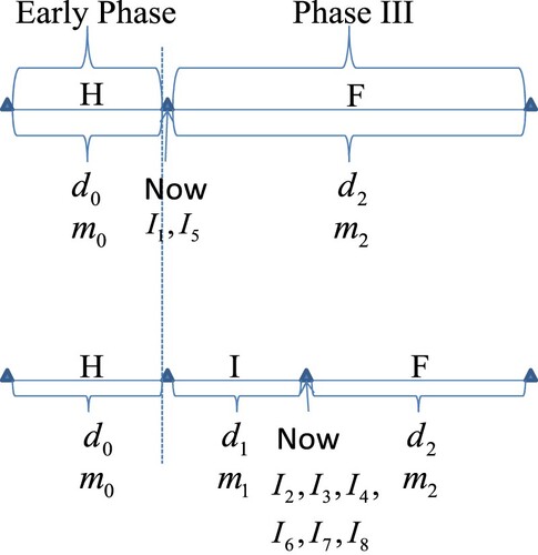
Figure 1. The data structures of the historical data, interim data and future data.

2. Eight predictive powers with historical and interim data

Similar to Dmitrienko and Wang (2006) and Jiang (2011), a go/no-go decision rule can be defined at the end of the early phase trial or at the interim of the Phase III trial. In our notation, (1) $\begin{array}{rl}& \mathrm{D}\mathrm{e}\mathrm{c}\mathrm{i}\mathrm{s}\mathrm{i}\mathrm{o}\mathrm{n}\mathrm{c}\mathrm{r}\mathrm{i}\mathrm{t}\mathrm{e}\mathrm{r}\mathrm{i}\mathrm{a}\\ & =\{\begin{array}{ll}\mathrm{S}\mathrm{t}\mathrm{o}\mathrm{p}\mathrm{f}\mathrm{o}\mathrm{r}\mathrm{e}\mathrm{f}\mathrm{f}\mathrm{i}\mathrm{c}\mathrm{a}\mathrm{c}\mathrm{y},& \mathrm{i}\mathrm{f}{\gamma }_e\le \mathrm{P}\mathrm{P},\\ \mathrm{G}\mathrm{o},& \mathrm{i}\mathrm{f}{\gamma }_g\le \mathrm{P}\mathrm{P}<{\gamma }_e,\\ \mathrm{C}\mathrm{o}\mathrm{n}\mathrm{d}\mathrm{i}\mathrm{t}\mathrm{i}\mathrm{o}\mathrm{n}\mathrm{a}\mathrm{l}-\mathrm{G}\mathrm{o},& \mathrm{i}\mathrm{f}{\gamma }_f<\mathrm{P}\mathrm{P}<{\gamma }_g,\\ \mathrm{S}\mathrm{t}\mathrm{o}\mathrm{p}\mathrm{f}\mathrm{o}\mathrm{r}\mathrm{f}\mathrm{u}\mathrm{t}\mathrm{i}\mathrm{l}\mathrm{i}\mathrm{t}\mathrm{y},& \mathrm{i}\mathrm{f}\mathrm{P}\mathrm{P}\le {\gamma }_f,\end{array}\end{array}$(1) where $\mathrm{P}\mathrm{P}$ is the predictive power, while ${\gamma }_f$, ${\gamma }_g$ and ${\gamma }_e$ are pre-specified thresholds for futility, go and efficacy, respectively. The thresholds should satisfy the following constraints: $0<{\gamma }_f<{\gamma }_g<{\gamma }_e<1.$Jiang (2011) suggests ${\gamma }_f\ge 0.5$, with ${\gamma }_f=0.5$ meaning that a stop for futility decision is taken if $1-\mathrm{P}\mathrm{P}\ge 0.5\ge \mathrm{P}\mathrm{P},$that is, the risk of failure is greater than or equal to the chance of success. The threshold ${\gamma }_e$ can be set at a relatively high value such as 0.9, so that when the $\mathrm{P}\mathrm{P}$ exceeds this threshold, a stop for efficacy decision can be made. Finally, the threshold ${\gamma }_g$ can be set at a value such as 0.8, so that if ${\gamma }_g\le \mathrm{P}\mathrm{P}<{\gamma }_e$, a go decision can be made, where ‘Go’ means moving on without the need of adjustment to the sample size of the future data $m_2$; if ${\gamma }_f<\mathrm{P}\mathrm{P}<{\gamma }_g$, a conditional-go decision can be made, where ‘Conditional-Go’  means moving on with the condition that $m_2$ is either increased to improve the $\mathrm{P}\mathrm{P}$ (so it is equal or close to ${\gamma }_g$) or staying unchanged while acknowledging a reduced $\mathrm{P}\mathrm{P}$ or increased risk of failure. Note that there are two no-go decisions in our decision criteria (1(1) $\begin{array}{rl}& \mathrm{D}\mathrm{e}\mathrm{c}\mathrm{i}\mathrm{s}\mathrm{i}\mathrm{o}\mathrm{n}\mathrm{c}\mathrm{r}\mathrm{i}\mathrm{t}\mathrm{e}\mathrm{r}\mathrm{i}\mathrm{a}\\ & =\{\begin{array}{ll}\mathrm{S}\mathrm{t}\mathrm{o}\mathrm{p}\mathrm{f}\mathrm{o}\mathrm{r}\mathrm{e}\mathrm{f}\mathrm{f}\mathrm{i}\mathrm{c}\mathrm{a}\mathrm{c}\mathrm{y},& \mathrm{i}\mathrm{f}{\gamma }_e\le \mathrm{P}\mathrm{P},\\ \mathrm{G}\mathrm{o},& \mathrm{i}\mathrm{f}{\gamma }_g\le \mathrm{P}\mathrm{P}<{\gamma }_e,\\ \mathrm{C}\mathrm{o}\mathrm{n}\mathrm{d}\mathrm{i}\mathrm{t}\mathrm{i}\mathrm{o}\mathrm{n}\mathrm{a}\mathrm{l}-\mathrm{G}\mathrm{o},& \mathrm{i}\mathrm{f}{\gamma }_f<\mathrm{P}\mathrm{P}<{\gamma }_g,\\ \mathrm{S}\mathrm{t}\mathrm{o}\mathrm{p}\mathrm{f}\mathrm{o}\mathrm{r}\mathrm{f}\mathrm{u}\mathrm{t}\mathrm{i}\mathrm{l}\mathrm{i}\mathrm{t}\mathrm{y},& \mathrm{i}\mathrm{f}\mathrm{P}\mathrm{P}\le {\gamma }_f,\end{array}\end{array}$(1) ), that is, stop for futility and stop for efficacy.

The data structures of the historical data, interim data and future data are described in Figure 1. In the figure, H means historical data, I means interim data and F means future data. The historical data could be the Phase II data, or the previous Phase III data, as long as the outcome variable and patient populations are the same between the historical data and the upcoming Phase III data. Moreover, the historical data could also be a fictitious data corresponding to a sceptical or optimistic prior, and in this case $d_0$ and $m_0$ of the historical data are determined to satisfy the requirements of the sceptical or optimistic prior. Note that $d_0$, $d_1$ and $d_2$ are the observed treatment differences in the treatment group and the control (or placebo) group of the historical data, interim data and future data respectively, and $m_0$, $m_1$ and $m_2$ are the per group number of patients of the historical data, interim data and future data respectively. In the upper plot, only historical data are available. Furthermore, the upper plot also depicts the data structure for  criterion (7(7) $\begin{array}{rl}& \{\begin{array}{l}{d}_2|\delta \sim N(\delta ,{\displaystyle \frac{2{\sigma }^2}{m_2}}),\\ \delta |d_0\sim N(d_0,{\displaystyle \frac{2{\sigma }^2}{m_0}}),\end{array}\\ & ⟹\{\begin{array}{l}\delta |d_0,d_2\sim N({\displaystyle \frac{m_0{d}_0+m_2{d}_2}{m_0+m_2}},{\displaystyle \frac{2{\sigma }^2}{m_0+m_2}}),\\ d_2|d_0\sim N(d_0,2{\sigma }^2({\displaystyle \frac{1}{m_0}}+{\displaystyle \frac{1}{m_2}})).\end{array}\end{array}$(7) ). Note that in the upper plot, the sample size of the future data $m_2$ is the whole sample size of the Phase III trial. Note that the present time of the program (termed now) in the upper plot is at the end of Early Phase and before the start of Phase III. At that time, only two predictive powers can be calculated to facilitate the go/no-go decision according to the decision criteria (1(1) $\begin{array}{rl}& \mathrm{D}\mathrm{e}\mathrm{c}\mathrm{i}\mathrm{s}\mathrm{i}\mathrm{o}\mathrm{n}\mathrm{c}\mathrm{r}\mathrm{i}\mathrm{t}\mathrm{e}\mathrm{r}\mathrm{i}\mathrm{a}\\ & =\{\begin{array}{ll}\mathrm{S}\mathrm{t}\mathrm{o}\mathrm{p}\mathrm{f}\mathrm{o}\mathrm{r}\mathrm{e}\mathrm{f}\mathrm{f}\mathrm{i}\mathrm{c}\mathrm{a}\mathrm{c}\mathrm{y},& \mathrm{i}\mathrm{f}{\gamma }_e\le \mathrm{P}\mathrm{P},\\ \mathrm{G}\mathrm{o},& \mathrm{i}\mathrm{f}{\gamma }_g\le \mathrm{P}\mathrm{P}<{\gamma }_e,\\ \mathrm{C}\mathrm{o}\mathrm{n}\mathrm{d}\mathrm{i}\mathrm{t}\mathrm{i}\mathrm{o}\mathrm{n}\mathrm{a}\mathrm{l}-\mathrm{G}\mathrm{o},& \mathrm{i}\mathrm{f}{\gamma }_f<\mathrm{P}\mathrm{P}<{\gamma }_g,\\ \mathrm{S}\mathrm{t}\mathrm{o}\mathrm{p}\mathrm{f}\mathrm{o}\mathrm{r}\mathrm{f}\mathrm{u}\mathrm{t}\mathrm{i}\mathrm{l}\mathrm{i}\mathrm{t}\mathrm{y},& \mathrm{i}\mathrm{f}\mathrm{P}\mathrm{P}\le {\gamma }_f,\end{array}\end{array}$(1) ), that is, the first and fifth predictive powers in Tables 1 and 2. If the $\mathrm{P}\mathrm{P}$ results in a ‘Go’ or ‘Conditional-Go’ decision according to the decision criteria (1(1) $\begin{array}{rl}& \mathrm{D}\mathrm{e}\mathrm{c}\mathrm{i}\mathrm{s}\mathrm{i}\mathrm{o}\mathrm{n}\mathrm{c}\mathrm{r}\mathrm{i}\mathrm{t}\mathrm{e}\mathrm{r}\mathrm{i}\mathrm{a}\\ & =\{\begin{array}{ll}\mathrm{S}\mathrm{t}\mathrm{o}\mathrm{p}\mathrm{f}\mathrm{o}\mathrm{r}\mathrm{e}\mathrm{f}\mathrm{f}\mathrm{i}\mathrm{c}\mathrm{a}\mathrm{c}\mathrm{y},& \mathrm{i}\mathrm{f}{\gamma }_e\le \mathrm{P}\mathrm{P},\\ \mathrm{G}\mathrm{o},& \mathrm{i}\mathrm{f}{\gamma }_g\le \mathrm{P}\mathrm{P}<{\gamma }_e,\\ \mathrm{C}\mathrm{o}\mathrm{n}\mathrm{d}\mathrm{i}\mathrm{t}\mathrm{i}\mathrm{o}\mathrm{n}\mathrm{a}\mathrm{l}-\mathrm{G}\mathrm{o},& \mathrm{i}\mathrm{f}{\gamma }_f<\mathrm{P}\mathrm{P}<{\gamma }_g,\\ \mathrm{S}\mathrm{t}\mathrm{o}\mathrm{p}\mathrm{f}\mathrm{o}\mathrm{r}\mathrm{f}\mathrm{u}\mathrm{t}\mathrm{i}\mathrm{l}\mathrm{i}\mathrm{t}\mathrm{y},& \mathrm{i}\mathrm{f}\mathrm{P}\mathrm{P}\le {\gamma }_f,\end{array}\end{array}$(1) ), then the Phase III trial is launched. However, if the $\mathrm{P}\mathrm{P}$ results in a no-go decision (either stop for futility or stop for efficacy), then the Phase III trial will not be launched. Furthermore, if the Phase III trial is launched and the interim data of the Phase III trial are available, the data structure of the program can be described in the lower plot of Figure 1. Note that the present time of the program (termed now) in the lower plot is at the interim of the Phase III trial. At the interim, there are six predictive powers which can be calculated to facilitate the go/no-go decision according to the decision criteria (1(1) $\begin{array}{rl}& \mathrm{D}\mathrm{e}\mathrm{c}\mathrm{i}\mathrm{s}\mathrm{i}\mathrm{o}\mathrm{n}\mathrm{c}\mathrm{r}\mathrm{i}\mathrm{t}\mathrm{e}\mathrm{r}\mathrm{i}\mathrm{a}\\ & =\{\begin{array}{ll}\mathrm{S}\mathrm{t}\mathrm{o}\mathrm{p}\mathrm{f}\mathrm{o}\mathrm{r}\mathrm{e}\mathrm{f}\mathrm{f}\mathrm{i}\mathrm{c}\mathrm{a}\mathrm{c}\mathrm{y},& \mathrm{i}\mathrm{f}{\gamma }_e\le \mathrm{P}\mathrm{P},\\ \mathrm{G}\mathrm{o},& \mathrm{i}\mathrm{f}{\gamma }_g\le \mathrm{P}\mathrm{P}<{\gamma }_e,\\ \mathrm{C}\mathrm{o}\mathrm{n}\mathrm{d}\mathrm{i}\mathrm{t}\mathrm{i}\mathrm{o}\mathrm{n}\mathrm{a}\mathrm{l}-\mathrm{G}\mathrm{o},& \mathrm{i}\mathrm{f}{\gamma }_f<\mathrm{P}\mathrm{P}<{\gamma }_g,\\ \mathrm{S}\mathrm{t}\mathrm{o}\mathrm{p}\mathrm{f}\mathrm{o}\mathrm{r}\mathrm{f}\mathrm{u}\mathrm{t}\mathrm{i}\mathrm{l}\mathrm{i}\mathrm{t}\mathrm{y},& \mathrm{i}\mathrm{f}\mathrm{P}\mathrm{P}\le {\gamma }_f,\end{array}\end{array}$(1) ), that is, the second, third, fourth, sixth, seventh and eighth predictive powers in Tables 1 and 2. In the lower plot, both historical data and interim data are available. Moreover, the lower plot also depicts the data structure for criterion (4(4) $\begin{array}{rl}& \{\begin{array}{l}{\displaystyle d_1|\delta \sim N(\delta ,\frac{2{\sigma }^2}{m_1}),}\\ {\displaystyle \delta |d_0\sim N(d_0,\frac{2{\sigma }^2}{m_0}),}\end{array}\\ & {\displaystyle ⟹\{\begin{array}{l}\delta |d_0,d_1\sim N(\frac{m_0{d}_0+m_1{d}_1}{m_0+m_1},\frac{2{\sigma }^2}{m_0+m_1}),\\ d_1|d_0\sim N(d_0,2{\sigma }^2(\frac{1}{m_0}+\frac{1}{m_1})).\end{array}}\end{array}$(4) ) and (5(5) $\begin{array}{rl}& \{\begin{array}{l}{\displaystyle d_2|\delta \sim N(\delta ,\frac{2{\sigma }^2}{m_2}),}\\ {\displaystyle \delta |d_0,d_1\sim N(\frac{m_0{d}_0+m_1{d}_1}{m_0+m_1},\frac{2{\sigma }^2}{m_0+m_1}),}\end{array}\\ & ⟹\\ & \{\begin{array}{l}{\displaystyle \delta |d_0,d_1,d_2\sim N(\frac{m_0{d}_0+m_1{d}_1+m_2{d}_2}{m_0+m_1+m_2},}\\ {\displaystyle \frac{2{\sigma }^2}{m_0+m_1+m_2}}),\\ {\displaystyle d_2|d_0,d_1\sim N(\frac{m_0{d}_0+m_1{d}_1}{m_0+m_1},2{\sigma }^2}\\ \times \left({\displaystyle \frac{1}{m_2}+\frac{1}{m_0+m_1}}\right)).\end{array}\end{array}$(5) ).

Note that F in the graph could be meaning data after interim in the lower plot, and full Phase III data in the upper plot. The justifications of the meaning of F are given as follows. First, the future data are the data after the present time (termed now in the upper and lower plots). Second, in the lower plot, when the information time increases, the interim data become more and more, and the future data become less and less. Conversely, when the information time decreases, the future data become more and more, and the interim data become less and less. When the information time is 0, the future data is the full Phase III data.

Suppose that the interim analysis of a randomized controlled Phase III trial is to be conducted with patients randomized to one of two treatments, with $m_1$ patients allocated to treatment i (i = 1, 2), where treatment 2 is the test drug and treatment 1 is the control (or placebo). Moreover, suppose that the j-th patient receiving treatment i for the interim data will yield a continuous response $x_{ij1}$ that we can assume is normally distributed with an unknown mean ${\mu }_{i1}$ and a common known variance ${\sigma }^2$. The third subscript ‘1’ in $x_{ij1}$ means that the responses are for the interim data. Moreover, assume that the data from the two treatments are independent. Thus the model of the interim data of the Phase III trial is that $x_{ij1}\stackrel{\mathrm{i}\mathrm{n}\mathrm{d}\mathrm{e}\mathrm{p}\mathrm{e}\mathrm{n}\mathrm{d}\mathrm{e}\mathrm{n}\mathrm{t}}{\sim }N({\mu }_{i1},{\sigma }^2),j=1,\dots ,m_1,i=1,2.$It is easy to derive the sampling distributions of the sufficient statistics $\begin{array}{rl}{\overline{x}}_{i1}|{\mu }_{i1}& =\left(\frac{1}{m_1}\sum _{j=1}^{m_1}{x}_{ij1}\right)|{\mu }_{i1}\\ & \sim N({\mu }_{i1},\frac{{\sigma }^2}{m_1}),i=1,2.\end{array}$More specifically, $\begin{array}{rl}& {\overline{x}}_{21}|{\mu }_{21}\sim N({\mu }_{21},\frac{{\sigma }^2}{m_1})\mathrm{a}\mathrm{n}\mathrm{d}\\ & {\overline{x}}_{11}|{\mu }_{11}\sim N({\mu }_{11},\frac{{\sigma }^2}{m_1}).\end{array}$Therefore, $d_1|\delta =({\overline{x}}_{21}-{\overline{x}}_{11})|\delta \sim N(\delta ,\frac{2{\sigma }^2}{m_1}),$where $d_1={\overline{x}}_{21}-{\overline{x}}_{11}$ is the sample mean difference based on the interim data of the Phase III trial, and $\delta ={\mu }_{21}-{\mu }_{11}$ is the true treatment effect based on the interim data of the Phase III trial.

Similarly, suppose that the future data of a randomized controlled Phase III trial is to be collected with patients randomized to one of two treatments, with $m_2$ patients allocated to each treatment. After some similar derivations for the interim analysis of the Phase III trial, we have $d_2|\delta \sim N(\delta ,\frac{2{\sigma }^2}{m_2}),$where $d_2={\overline{x}}_{22}-{\overline{x}}_{12}$ is the sample mean difference based on the future data of the Phase III trial, $\delta ={\mu }_{22}-{\mu }_{12}$ is the true treatment effect based on the future data of the Phase III trial, ${\overline{x}}_{i2}=\frac{1}{m_2}\sum _{j=1}^{m_2}{x}_{ij2}(i=1,2)$ is the sample mean of $x_{ij2}$ which is the continuous response of the j-th patient receiving treatment i for the future data, and ${\mu }_{i2}(i=1,2)$ is the unknown mean of $x_{ij2}$. The third subscript ‘2’ in $x_{ij2}$ means that the responses are for the future data. Note that we have assumed the true treatment effects based on the interim data and future data of the Phase III trial are the same. This assumption has also been used in the literature. See for instance (Spiegelhalter et al., 2004). Note also that the assumption can be easily violated in the clinical trials, such as the enrichment design which will change the population. Therefore, our discussions are not suitable for the enrichment design.

Suppose that we have some prior knowledge about δ through the historical data corresponding to $m_0$ patients per group in two treatments, and the prior mean of δ is estimated to be $d_0$. We remark that the historical data with $m_0$ patients refer to Phase II patients specifically, and thus the treatment effect δ in Phase II could be different than Phase III. However, in many disease areas where main clinical outcomes can be observed in relatively short duration – such as acute pain, allergy, asthma, depression, hypertension, and so on – Phase II and Phase III trials often have the same trial design including a same outcome variable and same patient population. In these disease areas, the treatment effect δ on Phase II and Phase III trials can be assumed the same. For simplicity, we assume a normal model for the prior. That is, (2) $\delta |d_0\sim N(d_0,\frac{2{\sigma }^2}{m_0}).$(2) Note that this prior incorporating the historical data can be obtained as follows. For the historical data $d_0$, assume that $d_0|\delta \sim N(\delta ,\frac{2{\sigma }^2}{m_0}).$Suppose that we have no prior knowledge about δ before the historical data $d_0$, and thus we assume that δ has an improper uniform prior over $(-\mathrm{\infty },\mathrm{\infty })$, that is, $\pi \left(\delta \right)\propto 1$. Then the posterior distribution of δ given $d_0$ is easily found to be given by (2(2) $\delta |d_0\sim N(d_0,\frac{2{\sigma }^2}{m_0}).$(2) ).

Therefore, when the interim data $d_1$ is available, the model and the prior are given by (3) $\begin{array}{rl}& d_1|\delta \sim N(\delta ,\frac{2{\sigma }^2}{m_1}),d_2|\delta \sim N(\delta ,\frac{2{\sigma }^2}{m_2}),\\ & \times \delta |d_0\sim N(d_0,\frac{2{\sigma }^2}{m_0}).\end{array}$(3) Let the model and prior be given by (3(3) $\begin{array}{rl}& d_1|\delta \sim N(\delta ,\frac{2{\sigma }^2}{m_1}),d_2|\delta \sim N(\delta ,\frac{2{\sigma }^2}{m_2}),\\ & \times \delta |d_0\sim N(d_0,\frac{2{\sigma }^2}{m_0}).\end{array}$(3) ). Given the likelihood $d_1|\delta$ and the prior $\delta |d_0$, standard Bayesian calculus yields the posterior distribution of δ given $d_0,d_1$ and the conditional distribution of $d_1$ given $d_0$, that is, (4) $\begin{array}{rl}& \{\begin{array}{l}{\displaystyle d_1|\delta \sim N(\delta ,\frac{2{\sigma }^2}{m_1}),}\\ {\displaystyle \delta |d_0\sim N(d_0,\frac{2{\sigma }^2}{m_0}),}\end{array}\\ & {\displaystyle ⟹\{\begin{array}{l}\delta |d_0,d_1\sim N(\frac{m_0{d}_0+m_1{d}_1}{m_0+m_1},\frac{2{\sigma }^2}{m_0+m_1}),\\ d_1|d_0\sim N(d_0,2{\sigma }^2(\frac{1}{m_0}+\frac{1}{m_1})).\end{array}}\end{array}$(4) Then using the posterior distribution $\pi (\delta |d_0,d_1)$ as a new prior for our future data $d_2$, standard Bayesian calculus yields the posterior distribution of δ given $d_0,d_1,d_2$ and the conditional distribution of $d_2$ given $d_0,d_1$, that is, (5) $\begin{array}{rl}& \{\begin{array}{l}{\displaystyle d_2|\delta \sim N(\delta ,\frac{2{\sigma }^2}{m_2}),}\\ {\displaystyle \delta |d_0,d_1\sim N(\frac{m_0{d}_0+m_1{d}_1}{m_0+m_1},\frac{2{\sigma }^2}{m_0+m_1}),}\end{array}\\ & ⟹\\ & \{\begin{array}{l}{\displaystyle \delta |d_0,d_1,d_2\sim N(\frac{m_0{d}_0+m_1{d}_1+m_2{d}_2}{m_0+m_1+m_2},}\\ {\displaystyle \frac{2{\sigma }^2}{m_0+m_1+m_2}}),\\ {\displaystyle d_2|d_0,d_1\sim N(\frac{m_0{d}_0+m_1{d}_1}{m_0+m_1},2{\sigma }^2}\\ \times \left({\displaystyle \frac{1}{m_2}+\frac{1}{m_0+m_1}}\right)).\end{array}\end{array}$(5) The data structure of (4(4) $\begin{array}{rl}& \{\begin{array}{l}{\displaystyle d_1|\delta \sim N(\delta ,\frac{2{\sigma }^2}{m_1}),}\\ {\displaystyle \delta |d_0\sim N(d_0,\frac{2{\sigma }^2}{m_0}),}\end{array}\\ & {\displaystyle ⟹\{\begin{array}{l}\delta |d_0,d_1\sim N(\frac{m_0{d}_0+m_1{d}_1}{m_0+m_1},\frac{2{\sigma }^2}{m_0+m_1}),\\ d_1|d_0\sim N(d_0,2{\sigma }^2(\frac{1}{m_0}+\frac{1}{m_1})).\end{array}}\end{array}$(4) ) and (5(5) $\begin{array}{rl}& \{\begin{array}{l}{\displaystyle d_2|\delta \sim N(\delta ,\frac{2{\sigma }^2}{m_2}),}\\ {\displaystyle \delta |d_0,d_1\sim N(\frac{m_0{d}_0+m_1{d}_1}{m_0+m_1},\frac{2{\sigma }^2}{m_0+m_1}),}\end{array}\\ & ⟹\\ & \{\begin{array}{l}{\displaystyle \delta |d_0,d_1,d_2\sim N(\frac{m_0{d}_0+m_1{d}_1+m_2{d}_2}{m_0+m_1+m_2},}\\ {\displaystyle \frac{2{\sigma }^2}{m_0+m_1+m_2}}),\\ {\displaystyle d_2|d_0,d_1\sim N(\frac{m_0{d}_0+m_1{d}_1}{m_0+m_1},2{\sigma }^2}\\ \times \left({\displaystyle \frac{1}{m_2}+\frac{1}{m_0+m_1}}\right)).\end{array}\end{array}$(5) ) is depicted in the lower plot of Figure 1. Note that the posterior distribution $\pi (\delta |d_0,d_1,d_2)$ is used in the calculations of the Bayesian rejection regions with $d_0,d_1,d_2$, $\begin{array}{rl}{S}_{\alpha ,{\delta }_0}^{B,d_0,d_1,d_2}& =\{P(\delta \le {\delta }_0|d_0,d_1,d_2)<\alpha \}\mathrm{a}\mathrm{n}\mathrm{d}\\ S_{\alpha ,{\delta }_0}^{B-,d_0,d_1,d_2}& =\{P(\delta \ge {\delta }_0|d_0,d_1,d_2)<\alpha \}.\end{array}$The conditional distribution $\pi (d_2|d_0,d_1)$ is the predictive distribution used in the calculations of the even-numbered predictive powers in Table 1.

Similarly, when the interim data $d_1$ is not available, the model and the prior are given by (6) $d_2|\delta \sim N(\delta ,\frac{2{\sigma }^2}{m_2}),\delta |d_0\sim N(d_0,\frac{2{\sigma }^2}{m_0}).$(6) Let the model and prior be given by (6(6) $d_2|\delta \sim N(\delta ,\frac{2{\sigma }^2}{m_2}),\delta |d_0\sim N(d_0,\frac{2{\sigma }^2}{m_0}).$(6) ). Given the likelihood $d_2|\delta$ and the prior $\delta |d_0$, standard Bayesian calculus yields the posterior distribution of δ given $d_0,d_2$ and the conditional distribution of $d_2$ given $d_0$, that is, (7) $\begin{array}{rl}& \{\begin{array}{l}{d}_2|\delta \sim N(\delta ,{\displaystyle \frac{2{\sigma }^2}{m_2}}),\\ \delta |d_0\sim N(d_0,{\displaystyle \frac{2{\sigma }^2}{m_0}}),\end{array}\\ & ⟹\{\begin{array}{l}\delta |d_0,d_2\sim N({\displaystyle \frac{m_0{d}_0+m_2{d}_2}{m_0+m_2}},{\displaystyle \frac{2{\sigma }^2}{m_0+m_2}}),\\ d_2|d_0\sim N(d_0,2{\sigma }^2({\displaystyle \frac{1}{m_0}}+{\displaystyle \frac{1}{m_2}})).\end{array}\end{array}$(7) The data structure of (7(7) $\begin{array}{rl}& \{\begin{array}{l}{d}_2|\delta \sim N(\delta ,{\displaystyle \frac{2{\sigma }^2}{m_2}}),\\ \delta |d_0\sim N(d_0,{\displaystyle \frac{2{\sigma }^2}{m_0}}),\end{array}\\ & ⟹\{\begin{array}{l}\delta |d_0,d_2\sim N({\displaystyle \frac{m_0{d}_0+m_2{d}_2}{m_0+m_2}},{\displaystyle \frac{2{\sigma }^2}{m_0+m_2}}),\\ d_2|d_0\sim N(d_0,2{\sigma }^2({\displaystyle \frac{1}{m_0}}+{\displaystyle \frac{1}{m_2}})).\end{array}\end{array}$(7) ) is depicted in the upper plot of Figure 1. Note that the posterior distribution $\pi (\delta |d_0,d_2)$ is used in the calculations of the Bayesian rejection regions with $d_0,d_2$, $\begin{array}{rl}{S}_{\alpha ,{\delta }_0}^{B,d_0,d_2}& =\{P(\delta \le {\delta }_0|d_0,d_2)<\alpha \}\mathrm{a}\mathrm{n}\mathrm{d}\\ S_{\alpha ,{\delta }_0}^{B-,d_0,d_2}& =\{P(\delta \ge {\delta }_0|d_0,d_2)<\alpha \}.\end{array}$The conditional distribution $\pi \left(d_2|d_0\right)$ is the predictive distribution used in the calculations of the odd-numbered predictive powers in Table 1.

For clarity, we define the Classical Power (CP), Classical Conditional Power (CCP), Bayesian Power (BP), and Bayesian Conditional Power (BCP). The CP is the probability of the classical rejection region with $d_2$, $S_{\alpha ,{\delta }_0}^{C,d_2}$, given a value for δ, $P\left(S_{\alpha ,{\delta }_0}^{C,d_2}|\delta \right)$, where S is for ‘Success’ and the success region is the rejection region, C is for ‘Classical’, α is the significance level, and ${\delta }_0$ is a threshold value for δ. The CCP is the probability of the classical rejection region with $d_1$ and $d_2$, $S_{\alpha ,{\delta }_0}^{C,d_1,d_2}$, given values of δ and interim result $d_1$, $P(S_{\alpha ,{\delta }_0}^{C,d_1,d_2}|\delta ,d_1)$. The BP is the probability of the Bayesian rejection region with $d_0,d_2$, $S_{\alpha ,{\delta }_0}^{B,d_0,d_2}$, given values of δ and historical result $d_0$, $P(S_{\alpha ,{\delta }_0}^{B,d_0,d_2}|\delta ,d_0)$, where B is for ‘Bayesian’. The BCP is the probability of the Bayesian rejection region with $d_0,d_1,d_2$, $S_{\alpha ,{\delta }_0}^{B,d_0,d_1,d_2}$, given values of $\delta ,d_0,d_1$, $P(S_{\alpha ,{\delta }_0}^{B,d_0,d_1,d_2}|\delta ,d_0,d_1)$. Under normality assumptions for the priors and the likelihoods, it is easy to obtain the expressions of the rejection regions and the powers as $\begin{array}{rl}{S}_{\alpha ,{\delta }_0}^{C,d_2}& =\{d_2>A\},\\ S_{\alpha ,{\delta }_0}^{C,d_1,d_2}& =\{d_2>B\left(d_1\right)\},\\ S_{\alpha ,{\delta }_0}^{B,d_0,d_2}& =\{d_2>C\left(d_0\right)\},\\ S_{\alpha ,{\delta }_0}^{B,d_0,d_1,d_2}& =\{d_2>D(d_0,d_1)\},\\ \mathrm{C}\mathrm{P}& =P\left(S_{\alpha ,{\delta }_0}^{C,d_2}|\delta \right)=\mathrm{\Phi }\left[\frac{\delta -A}{\sqrt{2/m_2}\sigma }\right],\\ \mathrm{C}\mathrm{C}\mathrm{P}& =P(S_{\alpha ,{\delta }_0}^{C,d_1,d_2}|\delta ,d_1)=\mathrm{\Phi }\left[\frac{\delta -B\left(d_1\right)}{\sqrt{2/m_2}\sigma }\right],\\ \mathrm{B}\mathrm{P}& =P(S_{\alpha ,{\delta }_0}^{B,d_0,d_2}|\delta ,d_0)=\mathrm{\Phi }\left[\frac{\delta -C\left(d_0\right)}{\sqrt{2/m_2}\sigma }\right],\\ \mathrm{B}\mathrm{C}\mathrm{P}& =P(S_{\alpha ,{\delta }_0}^{B,d_0,d_1,d_2}|\delta ,d_0,d_1)\\ & =\mathrm{\Phi }\left[\frac{\delta -D(d_0,d_1)}{\sqrt{2/m_2}\sigma }\right],\end{array}$where (8) $\begin{array}{rl}A& ={\delta }_0+Z_{\alpha }\sigma \sqrt{2/m_2},\end{array}$(8) (9) $\begin{array}{rl}B\left(d_1\right)& =\left[\frac{\begin{array}{c}(m_1+m_2){\delta }_0+Z_{\alpha }\sigma \sqrt{2(m_1+m_2)}-m_1{d}_1\end{array}}{m_2}\right],\end{array}$(9) (10) $\begin{array}{rl}C\left(d_0\right)& =\left[\frac{\begin{array}{c}(m_0+m_2){\delta }_0+Z_{\alpha }\sigma \sqrt{2(m_0+m_2)}-m_0{d}_0\end{array}}{m_2}\right],\end{array}$(10) (11) $\begin{array}{rl}D(d_0,d_1)& =\left[\frac{\begin{array}{c}(m_0+m_1+m_2){\delta }_0+Z_{\alpha }\sigma \sqrt{2(m_0+m_1+m_2)}-m_0{d}_0-m_1{d}_1\end{array}}{m_2}\right].\end{array}$(11) The detailed derivations of the expressions of the rejection regions and the powers can be found in the supplement.

Suppose that we are interested in testing the hypotheses $H_0:\delta \le {\delta }_0$ versus $H_1:\delta >{\delta }_0$. This kind of hypotheses arise when we assume that a larger value in the population mean of the normal distribution means improvement in disease condition. Hence, a positive value of δ means better. The eight predictive powers with historical and interim data, their analytical expressions, the predictive distributions, the data used, and the references for the hypotheses $H_0:\delta \le {\delta }_0$ versus $H_1:\delta >{\delta }_0$ are given in Table 1. Note that the definitions of the eight predictive powers for the hypotheses are given in Table 1 under the column name ‘Predictive Power’. In the table:

• For the predictive power column, $I_1$ is the Classical Predictive Power (CPP), $I_2$ is the Classical Interim Predictive Power (CIPP), $I_3$ is the Classical Conditional Predictive Power (CCPP), $I_4$ is the Classical Conditional Interim Predictive Power (CCIPP), $I_5$ is the Bayesian Predictive Power (BPP), $I_6$ is the Bayesian Interim Predictive Power (BIPP), $I_7$ is the Bayesian Conditional Predictive Power (BCPP) and $I_8$ is the Bayesian Conditional Interim Predictive Power (BCIPP). Now we explain our nomenclatures. Note that $P\left(S_{\alpha ,{\delta }_0}^{C,d_2}|\delta \right)$ is the Classical Power (CP), $P(S_{\alpha ,{\delta }_0}^{C,d_1,d_2}|\delta ,d_1)$ is the Classical Conditional Power (CCP), $P(S_{\alpha ,{\delta }_0}^{B,d_0,d_2}|\delta ,d_0)$ is the Bayesian Power (BP) and $P(S_{\alpha ,{\delta }_0}^{B,d_0,d_1,d_2}|\delta ,d_0,d_1)$ is the Bayesian Conditional Power (BCP). We add a capital letter P (short for Predictive) to the nomenclatures to indicate that they are predictive powers. Moreover, we add a capital letter I (short for Interim) to the nomenclatures to indicate that the prior $\pi (\delta |d_0,d_1)$ uses the interim data.

• The analytical expressions are given as follows: $\begin{array}{rl}{E}_1& =\mathrm{\Phi }\left[\frac{m_2(d_0-{\delta }_0)-Z_{\alpha }\sigma \sqrt{2m_2}}{\sqrt{2m_2}\sigma }\sqrt{\frac{m_0}{m_0+m_2}}\right],\\ E_2& =\mathrm{\Phi }\left[\frac{\begin{array}{c}{m}_0{m}_2(d_0-{\delta }_0)+m_1{m}_2(d_1-{\delta }_0)-Z_{\alpha }\sigma (m_0+m_1)\sqrt{2m_2}\end{array}}{\sqrt{2m_2}\sigma \sqrt{m_0+m_1}\sqrt{m_0+m_1+m_2}}\right],\\ E_3& =\mathrm{\Phi }\left[\sqrt{\frac{m_0}{m_0+m_2}}\frac{\begin{array}{c}{m}_1(d_1-{\delta }_0)+m_2(d_0-{\delta }_0)-Z_{\alpha }\sigma \sqrt{2(m_1+m_2)}\end{array}}{\sqrt{2m_2}\sigma }\right],\\ E_4& =\mathrm{\Phi }\left[\frac{\begin{array}{c}{m}_0{m}_2(d_0-{\delta }_0)+m_1(m_0+m_1+m_2)(d_1-{\delta }_0)-Z_{\alpha }\sigma (m_0+m_1)\sqrt{2(m_1+m_2)}\end{array}}{\sqrt{2m_2}\sigma \sqrt{m_0+m_1}\sqrt{m_0+m_1+m_2}}\right],\\ E_5& =\mathrm{\Phi }\left[\sqrt{\frac{m_0}{m_0+m_2}}\frac{\begin{array}{c}(m_0+m_2)(d_0-{\delta }_0)-Z_{\alpha }\sigma \sqrt{2(m_0+m_2)}\end{array}}{\sqrt{2m_2}\sigma }\right],\\ E_6& =\mathrm{\Phi }\left[\frac{\begin{array}{c}{m}_0(m_0+m_1+m_2)(d_0-{\delta }_0)+m_1{m}_2(d_1-{\delta }_0)-Z_{\alpha }\sigma (m_0+m_1)\sqrt{2(m_0+m_2)}\end{array}}{\sqrt{2m_2}\sigma \sqrt{m_0+m_1}\sqrt{m_0+m_1+m_2}}\right],\\ E_7& =\mathrm{\Phi }\left[\sqrt{\frac{m_0}{m_0+m_2}}\frac{\begin{array}{c}(m_0+m_2)(d_0-{\delta }_0)+m_1(d_1-{\delta }_0)-Z_{\alpha }\sigma \sqrt{2(m_0+m_1+m_2)}\end{array}}{\sqrt{2m_2}\sigma }\right],\\ E_8& =\mathrm{\Phi }\left[\frac{\begin{array}{c}(m_0+m_1+m_2)[m_0(d_0-{\delta }_0)+m_1(d_1-{\delta }_0)]-Z_{\alpha }\sigma (m_0+m_1)\sqrt{2(m_0+m_1+m_2)}\end{array}}{\sqrt{2m_2}\sigma \sqrt{m_0+m_1}\sqrt{m_0+m_1+m_2}}\right].\end{array}$

  Note that in the table, for $E_1$, $E_3$, $E_5$, and $E_7$, the analytical expressions are in the form of $\mathrm{\Phi }\left[\frac{d_0-\mathrm{E}\mathrm{x}\mathrm{p}\mathrm{r}\mathrm{e}\mathrm{s}\mathrm{s}\mathrm{i}\mathrm{o}\mathrm{n}}{\sqrt{2/m_2}\sigma }\sqrt{\frac{m_0}{m_0+m_2}}\right],$where the Expression is A, $B\left(d_1\right)$, $C\left(d_0\right)$ and $D(d_0,d_1)$ given by (8(8) $\begin{array}{rl}A& ={\delta }_0+Z_{\alpha }\sigma \sqrt{2/m_2},\end{array}$(8) ), (9(9) $\begin{array}{rl}B\left(d_1\right)& =\left[\frac{\begin{array}{c}(m_1+m_2){\delta }_0+Z_{\alpha }\sigma \sqrt{2(m_1+m_2)}-m_1{d}_1\end{array}}{m_2}\right],\end{array}$(9) ), (10(10) $\begin{array}{rl}C\left(d_0\right)& =\left[\frac{\begin{array}{c}(m_0+m_2){\delta }_0+Z_{\alpha }\sigma \sqrt{2(m_0+m_2)}-m_0{d}_0\end{array}}{m_2}\right],\end{array}$(10) ) and (11(11) $\begin{array}{rl}D(d_0,d_1)& =\left[\frac{\begin{array}{c}(m_0+m_1+m_2){\delta }_0+Z_{\alpha }\sigma \sqrt{2(m_0+m_1+m_2)}-m_0{d}_0-m_1{d}_1\end{array}}{m_2}\right].\end{array}$(11) ), respectively. Similarly, for $E_2$, $E_4$, $E_6$ and $E_8$, the analytical expressions are in the form of $\mathrm{\Phi }\left[\frac{m_0(d_0-\mathrm{E}\mathrm{x}\mathrm{p}\mathrm{r}\mathrm{e}\mathrm{s}\mathrm{s}\mathrm{i}\mathrm{o}\mathrm{n})+m_1(d_1-\mathrm{E}\mathrm{x}\mathrm{p}\mathrm{r}\mathrm{e}\mathrm{s}\mathrm{s}\mathrm{i}\mathrm{o}\mathrm{n})}{\sqrt{2/m_2}\sigma \sqrt{m_0+m_1}\sqrt{m_0+m_1+m_2}}\right],$where the Expression is A, $B\left(d_1\right)$, $C\left(d_0\right)$ and $D(d_0,d_1)$, respectively. The tedious calculations of the analytical expressions of the eight predictive powers in Table 1 can be found in the supplement. It is worth noting that the calculations of the predictive powers by directly calculating the expectations need an important expectation identity (Zhang et al., 2014, 2020b).

• Note that in the table, there are only two predictive distributions, that is, $\pi \left(d_2|d_0\right)$ and $\pi (d_2|d_0,d_1)$.

• For the data used column, H means that the historical data are used, and I means that the interim data are used. HI means that the historical data are used once and the interim data are also used once. HI${}^2$ means that the historical data are used once and the interim data are used twice. H${}^2$ means that the historical data are used twice. H${}^2$I means that the historical data are used twice and the interim data are used once. H${}^2$I${}^2$ means that the historical data are used twice and the interim data are also used twice. Now we explain why the eight predictive powers use different combination of historical and interim data. Note that the predictive power is an average power with respect to some priors. Only two priors are exploited for the eight predictive powers, that is, $\pi \left(\delta |d_0\right)$ and $\pi (\delta |d_0,d_1)$. The prior $\pi \left(\delta |d_0\right)$ uses the historical data ($d_0$) once. However, the prior $\pi (\delta |d_0,d_1)$ uses the historical data ($d_0$) once and the interim data ($d_1$) once. Four powers are used in the eight predictive powers, that is, the classical power $P\left(S_{\alpha ,{\delta }_0}^{C,d_2}|\delta \right)$ that does not use any data, the classical conditional power $P(S_{\alpha ,{\delta }_0}^{C,d_1,d_2}|\delta ,d_1)$ that uses the interim data once, the Bayesian power $P(S_{\alpha ,{\delta }_0}^{B,d_0,d_2}|\delta ,d_0)$ that uses the historical data once and the Bayesian conditional power $P(S_{\alpha ,{\delta }_0}^{B,d_0,d_1,d_2}|\delta ,d_0,d_1)$ that uses the historical data once and the interim data once. Therefore, for the predictive power $I_1$, it uses the historical data once, since it is an average classical power $P\left(S_{\alpha ,{\delta }_0}^{C,d_2}|\delta \right)$ with respect to the prior $\pi \left(\delta |d_0\right)$. Moreover, for the predictive power $I_8$, it uses the historical data twice and the interim data twice, since it is an average Bayesian conditional power $P(S_{\alpha ,{\delta }_0}^{B,d_0,d_1,d_2}|\delta ,d_0,d_1)$ with respect to the prior $\pi (\delta |d_0,d_1)$. The data used for other predictive powers can be explained in the same way.

• For $I_1$, $I_4$, $I_5$ and $I_8$, we can find a similar formula in Spiegelhalter et al. (2004). Note that in Spiegelhalter et al. (2004), the variance is ${\sigma }^2$ which corresponds to one arm trial, while in our article, the variance is $2{\sigma }^2$ which corresponds to two arm trials. The other four predictive powers ($I_2$, $I_3$, $I_6$ and $I_7$) are discovered by us. Consequently, Table 1 gives us a complete picture of the predictive powers with historical and interim data for futility and efficacy analysis for the hypotheses $H_0:\delta \le {\delta }_0$ versus $H_1:\delta >{\delta }_0$. Moreover, Spiegelhalter et al. (2004) use $z_{ϵ}$ which is a lower ϵ quantile, that is, $P(Z\le z_{ϵ})=ϵ$, while we use $Z_{\alpha }$ which is an upper α quantile, that is, $P(Z\ge Z_{\alpha })=\alpha$, and they have the simple relationship $z_{\alpha }=-Z_{\alpha }$.

Now suppose that we are interested in testing the reversed hypotheses $H_0:\delta \ge {\delta }_0$ versus $H_1:\delta <{\delta }_0$. This kind of hypotheses arise when we assume that a smaller value in the population of the normal distribution means improvement in disease condition. Hence, a negative value of δ means better. We will use a ‘−’ sign here to indicate that the respective quantities are calculated for the reversed hypotheses. The eight predictive powers with historical and interim data, their analytical expressions, the predictive distributions, and the data used for the reversed hypotheses $H_0:\delta \ge {\delta }_0$ versus $H_1:\delta <{\delta }_0$ are given in Table 2. Note that the definitions of the eight predictive powers for the reversed hypotheses are given in Table 2 under the column name ‘Predictive Power’. In the table:

• For the predictive power column, the nomenclatures are the same as in Table 1 with a ‘−’ sign here to indicate that the respective nomenclatures are for the reversed hypotheses.

• The analytical expressions are given as follows: $\begin{array}{rl}{E}_1^{-}& =\mathrm{\Phi }\left[\frac{-m_2(d_0-{\delta }_0)-Z_{\alpha }\sigma \sqrt{2m_2}}{\sqrt{2m_2}\sigma }\sqrt{\frac{m_0}{m_0+m_2}}\right],\\ E_2^{-}& =\mathrm{\Phi }\left[\frac{\begin{array}{c}-m_0{m}_2(d_0-{\delta }_0)-m_1{m}_2(d_1-{\delta }_0)-Z_{\alpha }\sigma (m_0+m_1)\sqrt{2m_2}\end{array}}{\sqrt{2m_2}\sigma \sqrt{m_0+m_1}\sqrt{m_0+m_1+m_2}}\right],\end{array}$ $\begin{array}{rl}{E}_3^{-}& =\mathrm{\Phi }\left[\sqrt{\frac{m_0}{m_0+m_2}}\frac{\begin{array}{c}-m_1(d_1-{\delta }_0)-m_2(d_0-{\delta }_0)-Z_{\alpha }\sigma \sqrt{2(m_1+m_2)}\end{array}}{\sqrt{2m_2}\sigma }\right],\\ E_4^{-}& =\mathrm{\Phi }\left[\frac{\begin{array}{c}-m_0{m}_2(d_0-{\delta }_0)-m_1(m_0+m_1+m_2)(d_1-{\delta }_0)-Z_{\alpha }\sigma (m_0+m_1)\sqrt{2(m_1+m_2)}\end{array}}{\sqrt{2m_2}\sigma \sqrt{m_0+m_1}\sqrt{m_0+m_1+m_2}}\right],\\ E_5^{-}& =\mathrm{\Phi }\left[\sqrt{\frac{m_0}{m_0+m_2}}\frac{\begin{array}{c}-(m_0+m_2)(d_0-{\delta }_0)-Z_{\alpha }\sigma \sqrt{2(m_0+m_2)}\end{array}}{\sqrt{2m_2}\sigma }\right],\\ E_6^{-}& =\mathrm{\Phi }\left[\frac{\begin{array}{c}-m_0(m_0+m_1+m_2)(d_0-{\delta }_0)-m_1{m}_2(d_1-{\delta }_0)-Z_{\alpha }\sigma (m_0+m_1)\sqrt{2(m_0+m_2)}\end{array}}{\sqrt{2m_2}\sigma \sqrt{m_0+m_1}\sqrt{m_0+m_1+m_2}}\right],\\ E_7^{-}& =\mathrm{\Phi }\left[\sqrt{\frac{m_0}{m_0+m_2}}\frac{\begin{array}{c}-(m_0+m_2)(d_0-{\delta }_0)-m_1(d_1-{\delta }_0)-Z_{\alpha }\sigma \sqrt{2(m_0+m_1+m_2)}\end{array}}{\sqrt{2m_2}\sigma }\right],\\ E_8^{-}& =\mathrm{\Phi }\left[\frac{\begin{array}{c}{m}_0(m_0+m_1+m_2)[-m_0(d_0-{\delta }_0)-m_1(d_1-{\delta }_0)]-Z_{\alpha }\sigma (m_0+m_1)\sqrt{2(m_0+m_1+m_2)}\end{array}}{\sqrt{2m_2}\sigma \sqrt{m_0+m_1}\sqrt{m_0+m_1+m_2}}\right].\end{array}$Note that in the table, for $E_1^{-}$, $E_3^{-}$, $E_5^{-}$ and $E_7^{-}$, the analytical expressions are in the form of $\mathrm{\Phi }\left[\frac{\mathrm{E}\mathrm{x}\mathrm{p}\mathrm{r}\mathrm{e}\mathrm{s}\mathrm{s}\mathrm{i}\mathrm{o}\mathrm{n}-d_0}{\sqrt{2/m_2}\sigma }\sqrt{\frac{m_0}{m_0+m_2}}\right],$where the Expression is $\begin{array}{rl}{A}^{-}& ={\delta }_0-Z_{\alpha }\sigma \sqrt{2/m_2},\\ B^{-}\left(d_1\right)& =\left[\frac{(m_1+m_2){\delta }_0-Z_{\alpha }\sigma \sqrt{2(m_1+m_2)}-m_1{d}_1}{m_2}\right],\\ C^{-}\left(d_0\right)& =\left[\frac{(m_0+m_2){\delta }_0-Z_{\alpha }\sigma \sqrt{2(m_0+m_2)}-m_0{d}_0}{m_2}\right],\\ D^{-}(d_0,d_1)& =\left[\frac{(m_0+m_1+m_2){\delta }_0-Z_{\alpha }\sigma \sqrt{2(m_0+m_1+m_2)}-m_0{d}_0-m_1{d}_1}{m_2}\right],\end{array}$respectively. Similarly, for $E_2^{-}$, $E_4^{-}$, $E_6^{-}$ and $E_8^{-}$, the analytical expressions are in the form of $\mathrm{\Phi }\left[\frac{m_0(\mathrm{E}\mathrm{x}\mathrm{p}\mathrm{r}\mathrm{e}\mathrm{s}\mathrm{s}\mathrm{i}\mathrm{o}\mathrm{n}-d_0)+m_1(\mathrm{E}\mathrm{x}\mathrm{p}\mathrm{r}\mathrm{e}\mathrm{s}\mathrm{s}\mathrm{i}\mathrm{o}\mathrm{n}-d_1)}{\sqrt{2/m_2}\sigma \sqrt{m_0+m_1}\sqrt{m_0+m_1+m_2}}\right],$where the Expression is $A^{-}$, $B^{-}\left(d_1\right)$, $C^{-}\left(d_0\right)$ and $D^{-}(d_0,d_1)$, respectively. The tedious calculations of the analytical expressions of the eight predictive powers in Table 2 can be found in the supplement.

• Note that in the table, there are only two predictive distributions, that is, $\pi \left(d_2|d_0\right)$ and $\pi (d_2|d_0,d_1)$.

• The data used column can be explained in the same way as in Table 1.

• There are no references available to the best of our knowledge for the reversed hypotheses $H_0:\delta \ge {\delta }_0$ versus $H_1:\delta <{\delta }_0$.

Comparing Tables 1 and 2, we find that for each predictive power, the predictive distribution and the data used are the same. From the two tables we see that the analytical expressions of the hypotheses $H_0:\delta \ge {\delta }_0$ versus $H_1:\delta <{\delta }_0$ are just the quantities of the hypotheses $H_0:\delta \le {\delta }_0$ versus $H_1:\delta >{\delta }_0$ with the terms involving $d_0-{\delta }_0$ and $d_1-{\delta }_0$ adding a negative sign, and vice versa.

3. A real data example

Long-term tamoxifen therapy is used for the prevention of recurrence of breast cancer (see Dignam et al., 1998; Example 6.7 in Spiegelhalter et al., 2004). The aim of the study is to estimate disease-free survival benefit from tamoxifen over placebo, in patients who already have had 5 years of taking tamoxifen without a recurrence. That means, patients were randomized to either continuation of tamoxifen therapy or continuation with placebo after having survived recurrence-free under tamoxifen for 5 years. To detect a $40\mathrm{\%}$ reduction in annual risk associated with tamoxifen (hazard ratio $=0.6$), with $85\mathrm{\%}$ power and a one-sided tail area of $5\mathrm{\%}$, 115 events were required. The statistical model is the proportional hazards regression model, with summary using the approximate hazard ratio analysis. If there are $O_T$ events on treatment, and $O_C$ events on control, then $d_1=2(O_T-O_C)/m_1$ is an approximate estimate of the log(hazard ratio) δ, with mean δ and variance $4/m_1$, as shown in Tsiatis (1981). Prior distributions: an optimistic prior was centred on a $40\mathrm{\%}$ hazard reduction and a $5\mathrm{\%}$ chance of a negative effect (i.e., HR>1), equivalent on the $\log \left(\mathrm{H}\mathrm{R}\right)$ scale to a normal prior with mean ${\mu }_o=\log \left(0.6\right)=-0.51$ and standard deviation 0.31 ($\sigma =\sqrt{2}$, $m_0\approx 41.4$). Note that in Spiegelhalter et al. (2004), the variance is ${\sigma }^2=4$, while in our article, the variance is $2{\sigma }^2=4$, and thus $\sigma =\sqrt{2}$ in our article. Moreover, $m_0\approx 41.4$ is used to guarantee that ‘an optimistic prior was centred on a $40\mathrm{\%}$ hazard reduction and a $5\mathrm{\%}$ chance of a negative effect’. Also a sceptical prior was adopted with the same standard deviation as the optimistic prior but centred on ${\mu }_s=0$. The estimated $\log \left(\mathrm{H}\mathrm{R}\right)$ after the first interim analysis in 1993 is $d_1=0.435$. At that time $m_1=46$ events have been observed, and further $m_2=115-46=69$ events are to be observed.

In the tamoxifen example, let $h_1$ and $h_2$ be the hazard rates corresponding to tamoxifen (treatment) and placebo (control) respectively. Therefore, $\begin{array}{rl}\mathrm{T}\mathrm{a}\mathrm{m}\mathrm{o}\mathrm{x}\mathrm{i}\mathrm{f}\mathrm{e}\mathrm{n}\mathrm{s}\mathrm{u}\mathrm{p}\mathrm{e}\mathrm{r}\mathrm{i}\mathrm{o}\mathrm{r}& \iff h_1<h_2\iff \mathrm{H}\mathrm{R}=\frac{h_1}{h_2}\\ & <1\iff \delta =\log \left(\mathrm{H}\mathrm{R}\right)<0,\\ \mathrm{C}\mathrm{o}\mathrm{n}\mathrm{t}\mathrm{r}\mathrm{o}\mathrm{l}\mathrm{s}\mathrm{u}\mathrm{p}\mathrm{e}\mathrm{r}\mathrm{i}\mathrm{o}\mathrm{r}& \iff h_1>h_2\iff \mathrm{H}\mathrm{R}=\frac{h_1}{h_2}\\ & >1\iff \delta =\log \left(\mathrm{H}\mathrm{R}\right)>0.\end{array}$Consequently, for $j=1,\dots ,8$, the j-th predictive power $I_j$ is for control superior, the j-th predictive power $I_j^{-}$ is for tamoxifen superior, and $1-I_j-I_j^{-}$ is for equivocal.

The eight predictive powers with historical and interim data of eventual conclusions for the B-14 trial after the first interim analysis in 1993 are reported in Table 3. In the table, the conclusion is: ‘Tamoxifen superior’, defined as a $1-\alpha$ confidence interval or credible interval for $\delta =\log \left(\mathrm{H}\mathrm{R}\right)$ lying wholly below 0; ‘Equivocal’, defined as a $1-2\alpha$ confidence interval or credible interval for $\delta =\log \left(\mathrm{H}\mathrm{R}\right)$ including 0; and ‘Control superior’, defined as a $1-\alpha$ confidence interval or credible interval for $\delta =\log \left(\mathrm{H}\mathrm{R}\right)$ lying wholly above 0. The significance level α is chosen to be 0.025 in all cases. For the first and fifth predictive powers, the number of events of the future data $m_2$ is the whole number of events of the Phase III trial 115, not 69 (the further number of events to be observed). In Table 3, we observe the following facts.

Table 3. The eight predictive powers with historical and interim data of eventual conclusions for the B-14 trial after the first interim analysis in 1993. Two prior distributions are considered: a sceptical prior and an optimistic prior.

	Tamoxifen superior		Equivocal		Control superior
No.	Sceptical	Optimistic	Sceptical	Optimistic	Sceptical	Optimistic
1	0.156	0.656	0.687	0.336	0.156	0.008
2	0.015	0.077	0.760	0.857	0.225	0.066
3	0.011	0.161	0.781	0.821	0.208	0.017
4	0.000	0.003	0.610	0.846	0.389	0.151
5	0.120	0.771	0.761	0.228	0.120	0.001
6	0.005	0.195	0.869	0.803	0.126	0.002
7	0.005	0.321	0.852	0.678	0.142	0.001
8	0.000	0.017	0.724	0.972	0.276	0.011

• The sum of the three predictive powers in each row corresponding to the sceptical prior (or the optimistic prior) should be equal to 1. However, in some cases, the sum is equal to 0.999, due to the rounding error.

• The fourth predictive powers in Table 3 are the same as those under the column ‘When not using prior in analysis’, which can be calculated by (6.15), in Table 6.7 of Spiegelhalter et al. (2004). Moreover, the eighth predictive powers in Table 3 are the same as those under the column ‘When using prior in analysis’, which can be calculated by (6.18), in Table 6.7 of Spiegelhalter et al. (2004).

• All the predictive powers under the ‘Tamoxifen superior’ column are less than 0.85, the designed power. Note that these predictive powers are calculated when the significance level α is chosen to be 0.025, while the designed power 0.85 is calculated when α is chosen to be 0.05. When the significance level α is risen to 0.05 when calculating the predictive powers, the predictive powers also rise, as the predictive powers are increasing functions of α. However, they are still less than 0.85. This phenomenon has been observed in the literature. See for instance Chuang-Stein (2006); Chuang-Stein Kirby (2017); Spiegelhalter et al. (2004).

• For the eight predictive powers, the optimistic prior has a greater tendency to draw a ‘Tamoxifen superior’  conclusion than the sceptical prior, and this is reflected in the predictive powers. In contrast, the sceptical prior has a greater tendency to draw a ‘Control superior’ conclusion than the optimistic prior, and this is also reflected in the predictive powers.

• Now let us focus on the ‘Tamoxifen superior’ column. The first predictive power under the optimistic prior is 0.656, which is fairly high, due to the first predictive power only uses the historical data once and it does not use the interim data, and the historical data (a fictitious data corresponding to the optimistic prior) favours the tamoxifen treatment. The fifth predictive power under the optimistic prior is 0.771, which is even higher, due to the fifth predictive power uses the historical data twice and it does not use the interim data, and the historical data favours the tamoxifen treatment. Note that the time point of the first and fifth predictive powers is before the launch of the Phase III trial. Since the first and fifth predictive powers are between ${\gamma }_f=0.5$ and ${\gamma }_g=0.8$ in the decision criteria (1(1) $\begin{array}{rl}& \mathrm{D}\mathrm{e}\mathrm{c}\mathrm{i}\mathrm{s}\mathrm{i}\mathrm{o}\mathrm{n}\mathrm{c}\mathrm{r}\mathrm{i}\mathrm{t}\mathrm{e}\mathrm{r}\mathrm{i}\mathrm{a}\\ & =\{\begin{array}{ll}\mathrm{S}\mathrm{t}\mathrm{o}\mathrm{p}\mathrm{f}\mathrm{o}\mathrm{r}\mathrm{e}\mathrm{f}\mathrm{f}\mathrm{i}\mathrm{c}\mathrm{a}\mathrm{c}\mathrm{y},& \mathrm{i}\mathrm{f}{\gamma }_e\le \mathrm{P}\mathrm{P},\\ \mathrm{G}\mathrm{o},& \mathrm{i}\mathrm{f}{\gamma }_g\le \mathrm{P}\mathrm{P}<{\gamma }_e,\\ \mathrm{C}\mathrm{o}\mathrm{n}\mathrm{d}\mathrm{i}\mathrm{t}\mathrm{i}\mathrm{o}\mathrm{n}\mathrm{a}\mathrm{l}-\mathrm{G}\mathrm{o},& \mathrm{i}\mathrm{f}{\gamma }_f<\mathrm{P}\mathrm{P}<{\gamma }_g,\\ \mathrm{S}\mathrm{t}\mathrm{o}\mathrm{p}\mathrm{f}\mathrm{o}\mathrm{r}\mathrm{f}\mathrm{u}\mathrm{t}\mathrm{i}\mathrm{l}\mathrm{i}\mathrm{t}\mathrm{y},& \mathrm{i}\mathrm{f}\mathrm{P}\mathrm{P}\le {\gamma }_f,\end{array}\end{array}$(1) ), a ‘Conditional-Go’ decision is made and the Phase III trial is launched. When the first interim data are available in 1993, we can calculate the other six predictive powers which use both the historical data and the interim data. Intuitively, when the interim data are available, they should be used to give a more accurate prediction. The interim data $d_1=0.435>0$ favours the control treatment. The combination of the historical data and the interim data produces the six predictive powers 0.077, 0.161, 0.003, 0.195, 0.321 and 0.017. The largest one of the six predictive powers is 0.321, corresponding to the seventh predictive power, which uses the historical data twice and the interim data once. At the same time, the seventh predictive power in favour of control and equivocal is as high as 0.679. The predictive powers in favour of tamoxifen under the sceptical prior are much lower than 0.321. Since the six predictive powers with interim data under the optimistic prior or the sceptical prior are all less than ${\gamma }_f=0.5$, according to the decision criteria (1(1) $\begin{array}{rl}& \mathrm{D}\mathrm{e}\mathrm{c}\mathrm{i}\mathrm{s}\mathrm{i}\mathrm{o}\mathrm{n}\mathrm{c}\mathrm{r}\mathrm{i}\mathrm{t}\mathrm{e}\mathrm{r}\mathrm{i}\mathrm{a}\\ & =\{\begin{array}{ll}\mathrm{S}\mathrm{t}\mathrm{o}\mathrm{p}\mathrm{f}\mathrm{o}\mathrm{r}\mathrm{e}\mathrm{f}\mathrm{f}\mathrm{i}\mathrm{c}\mathrm{a}\mathrm{c}\mathrm{y},& \mathrm{i}\mathrm{f}{\gamma }_e\le \mathrm{P}\mathrm{P},\\ \mathrm{G}\mathrm{o},& \mathrm{i}\mathrm{f}{\gamma }_g\le \mathrm{P}\mathrm{P}<{\gamma }_e,\\ \mathrm{C}\mathrm{o}\mathrm{n}\mathrm{d}\mathrm{i}\mathrm{t}\mathrm{i}\mathrm{o}\mathrm{n}\mathrm{a}\mathrm{l}-\mathrm{G}\mathrm{o},& \mathrm{i}\mathrm{f}{\gamma }_f<\mathrm{P}\mathrm{P}<{\gamma }_g,\\ \mathrm{S}\mathrm{t}\mathrm{o}\mathrm{p}\mathrm{f}\mathrm{o}\mathrm{r}\mathrm{f}\mathrm{u}\mathrm{t}\mathrm{i}\mathrm{l}\mathrm{i}\mathrm{t}\mathrm{y},& \mathrm{i}\mathrm{f}\mathrm{P}\mathrm{P}\le {\gamma }_f,\end{array}\end{array}$(1) ), we should stop the trial for futility.

4. Numerical simulations

In this section, we will conduct extensive simulations to investigate the sensitivity analysis of priors ($d_0$), sample sizes ($m_0$, $m_1$, $m_2$), interim result ($d_1$), and interim time (t) on the eight predictive powers. We assume that $\begin{array}{rl}\alpha & =0.025,{\delta }_0=0,\sigma =\sqrt{2},{\mu }_s=0,\\ {\mu }_o& =\log \left(0.6\right)\approx -0.51,\\ m_0^r& \approx 41.4,m_1^r=46,\\ m_2^r& =\{\begin{array}{ll}s=115,& \mathrm{f}\mathrm{o}\mathrm{r}i=1,5,\\ 69,& \mathrm{f}\mathrm{o}\mathrm{r}i=2,3,4,6,7,8,\end{array}\\ d_1^r& =0.435,s=115,t^r=\frac{m_1^r}{s}=0.4,\end{array}$where $m_0^r={\left(\frac{{\mathrm{\Phi }}^{-1}\left(0.05\right)\sqrt{2}\sigma }{{\mu }_o}\right)}^2\approx 41.4,$is calculated to ensure that an optimistic prior was centred on a $40\mathrm{\%}$ hazard reduction and a $5\mathrm{\%}$ chance of a negative effect (i.e., HR>1), equivalent on the $\log \left(\mathrm{H}\mathrm{R}\right)$ scale to a normal prior with mean ${\mu }_o=\log \left(0.6\right)\approx -0.51$ and standard deviation 0.31 ($\sigma =\sqrt{2}$, $m_0^r\approx 41.4$). We add a superscript ‘r’ in $m_0^r$, $m_1^r$, $m_2^r$, $d_1^r$ and $t^r$ to indicate that they are from the real data.

Now let us explain the special reason for choosing $\sigma =\sqrt{2}$ in the simulations section. As described in Section 2.4.2 in Spiegelhalter et al. (2004), suppose that the first intervention corresponds to an active treatment T, and the second to a control C. Often the results of a survival analysis may be given in terms of an observed log-rank test statistic $L_m$, which is defined as the excess of events under T, compared to that expected were there no treatment effect, where m is the total number of events observed. $L_m$ is often denoted as O−E (observed minus expected). Assuming proportional hazards, we have the following approximation in the particular case of equal allocation and follow-up. If there have been $O_T$ events on treatment, and $O_C$ events on control, then the expected number of events in the treatment group under the null hypothesis is approximately m/2, and hence the log-rank statistic is $L_m=O_T-m/2=(O_T-O_C)/2$. It can be shown in Tsiatis (1981) that, for large trials, $y_m=4L_m/m=2(O_T-O_C)/m$ is an approximate estimate of the log(hazard ratio) θ, and $y_m\sim N(\theta ,\frac{4}{m})=N(\theta ,\frac{{\sigma }^2}{m}).$Hence we can set $\sigma =2$ and adopt a normal likelihood. Note that in Spiegelhalter et al. (2004), the variance is ${\sigma }^2=4$, while in our article, the variance is $2{\sigma }^2=4$, and thus $\sigma =\sqrt{2}$ in our article, as $d_1=\frac{2(O_T-O_C)}{m_1}\sim N(\delta ,\frac{4}{m_1})=N(\delta ,\frac{2{\sigma }^2}{m_1}).$Let us introduce some notations used in this section. $I_i^{-}$ is the i-th predictive power for tamoxifen superior, $I_i$ is the i-th predictive power for control superior, and $1-I_i^{-}-I_i$ is the i-th predictive power for equivocal, for $i=1,\dots ,8$. $I_i^{s-}$ is the i-th predictive power of the sceptical prior for tamoxifen superior, $I_i^s$ is the i-th predictive power of the sceptical prior for control superior, $E_i^s=1-I_i^{s-}-I_i^s$ is the i-th predictive power of the sceptical prior for equivocal, $I_i^{o-}$ is the i-th predictive power of the optimistic prior for tamoxifen superior, $I_i^o$ is the i-th predictive power of the optimistic prior for control superior, and $E_i^o=1-I_i^{o-}-I_i^o$ is the i-th predictive power of the optimistic prior for equivocal, for $i=1,\dots ,8$. In the notations ($I_i^{s-}$, $I_i^s$, $E_i^s=1-I_i^{s-}-I_i^s$, $I_i^{o-}$, $I_i^o$ and $E_i^o=1-I_i^{o-}-I_i^o$), the superscript ‘s’ is for the sceptical prior which corresponds to $d_0={\mu }_s$, the superscript ‘o’ is for the optimistic prior which corresponds to $d_0={\mu }_o$, the subscript ‘i’ is for the i-th predictive power, $I^{-}$ is for tamoxifen superior, I is for control superior, and E is equivocal.

The sensitivity analysis of $d_0$ on the eight predictive powers is displayed in Figure 2. In the figure, we note the following issues.

Figure 2. The sensitivity analysis of $d_0$ on the eight predictive powers.

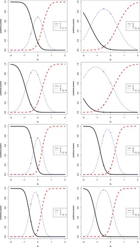
• The first and second predictive powers are related to the CP, the third and fourth predictive powers are related to the CCP, the fifth and sixth predictive powers are related to the BP, and the seventh and eighth predictive powers are related to the BCP.

• A negative $d_0$ favours tamoxifen, a positive $d_0$ favours control, and a $d_0$ near 0 favours equivocal.

• From the first plot, we see that $I_1^{-}$ is a decreasing function of $d_0$, $I_1$ is an increasing function of $d_0$, and $1-I_1^{-}-I_1$ is a first increasing and then decreasing function of $d_0$. The increase–decrease characteristics of $I_1^{-}$, $I_1$ and $1-I_1^{-}-I_1$ are compatible with the sign of $d_0$, as a negative $d_0$ favours tamoxifen and $I_1^{-}$ (the predictive power for tamoxifen superior) has a large value, a positive $d_0$ favours control and $I_1$ (the predictive power for control superior) has a large value, and a $d_0$ near 0 favours equivocal and $1-I_1^{-}-I_1$ (the predictive power for equivocal) has a large value.

• In the first plot, there are six markers labelled °, △, +, ×, ⋄ and ▽, which correspond to $({\mu }_s,I_1^{s-})$, $({\mu }_o,I_1^{o-})$, $({\mu }_s,E_1^s)$, $({\mu }_o,E_1^o)$, $({\mu }_s,I_1^s)$ and $({\mu }_o,I_1^o)$, respectively.

• In the first plot, the six values $I_1^{s-}$, $I_1^{o-}$, $E_1^s$, $E_1^o$, $I_1^s$ and $I_1^o$ are 0.156, 0.656, 0.687, 0.336, 0.156 and 0.008, which are the values in the first row of Table 3. The three values $I_1^{s-}=0.156$, $E_1^s=0.687$ and $I_1^s=0.156$ corresponding to $d_0={\mu }_s$ are for the sceptical prior, and the three values sum to 1 (in fact 0.999, due to the rounding error). Moreover, the three values $I_1^{o-}=0.656$, $E_1^o=0.336$ and $I_1^o=0.008$ corresponding to $d_0={\mu }_o$ are for the optimistic prior, and the three values sum to 1.

• The predictive powers $(I_i^{s-},I_i^{o-},E_i^s,E_i^o,I_i^s,I_i^o)$ for $i=1,\dots ,8$ in Table 3 are labelled in the figure by the six markers °, △, +, ×, ⋄ and ▽.

• In the first plot, a different $d_0$ value corresponds to a different prior, with $d_0={\mu }_s$ corresponding to the sceptical prior, and $d_0={\mu }_o$ corresponding to the optimistic prior.

• From the first plot, we see that as $d_0$ moves from ${\mu }_s=0$ to ${\mu }_o=\log \left(0.6\right)\approx -0.51$ and to below ${\mu }_o$, the $d_0$ values favour tamoxifen more and more, and the predictive powers for tamoxifen superior ($I_1^{-}$) are becoming larger and larger, while the predictive powers for control superior ($I_1$) and equivocal ($1-I_1^{-}-I_1$) are getting smaller and smaller. Conversely, as $d_0$ moves from ${\mu }_s=0$ to above ${\mu }_s$, the $d_0$ values favour control more and more, and the predictive powers for control superior ($I_1$) are becoming larger and larger, while the predictive powers for tamoxifen superior ($I_1^{-}$) and equivocal ($1-I_1^{-}-I_1$) are getting smaller and smaller.

• The other seven plots can be explained similarly to the first plot.

• It is interesting to note that for the first and fifth predictive powers, the predictive powers for equivocal are symmetric around $d_0=0$, and thus when $d_0$ moves from ${\mu }_s=0$ to ${\mu }_o=\log \left(0.6\right)\approx -0.51$, the predictive powers for equivocal are getting smaller and smaller. While for the other six predictive powers, the predictive powers for equivocal are symmetric around a negative $d_0$, and thus when $d_0$ moves from ${\mu }_s=0$ to ${\mu }_o=\log \left(0.6\right)\approx -0.51$, the predictive powers for equivocal may get bigger and bigger (e.g., the second, fourth and eighth predictive powers), or may get bigger and then smaller (e.g., the third, sixth and seventh predictive powers).

The sensitivity analysis of $m_0$ on the eight predictive powers is displayed in Figure 3. In the figure, we note the following issues.

• For the i-th ($i=1,\dots ,8$) predictive power, there are six markers labelled °, △, +, ×, ⋄ and ▽, which correspond to $(m_0^r,I_i^{s-})$, $(m_0^r,I_i^{o-})$, $(m_0^r,E_i^s)$, $(m_0^r,E_i^o)$, $(m_0^r,I_i^s)$ and $(m_0^r,I_i^o)$, respectively. The predictive powers $(I_i^{s-},I_i^{o-},E_i^s,E_i^o,I_i^s,I_i^o)$ for $i=1,\dots ,8$ in Table 3 are labelled in the figure by the six markers °, △, +, ×, ⋄ and ▽.

• Note that $\mathrm{V}\mathrm{a}\mathrm{r}\left(d_0|\delta \right)=2{\sigma }^2/m_0$, and thus when $m_0$ is large, the variance of $d_0|\delta$ will be small.

• The increase-decrease characteristics of $I_i^{s-}$, $I_i^s$, $1-I_i^{s-}-I_i^s$, $I_i^{o-}$, $I_i^o$ and $1-I_i^{o-}-I_i^o$ for $i=1,\dots ,8$ observed from Figure 3 are summarized in Table 4. From the table, we observe that as $m_0$ increases, $I_i^s$ decrease, $1-I_i^{s-}-I_i^s$ increase, and $I_i^o$ decrease for all eight predictive powers. $I_i^{s-}$ are decreasing functions of $m_0$ for the odd-numbered predictive powers, and they are zero constants for the even-numbered predictive powers. For $I_i^{o-}$, they are increasing functions of $m_0$ for the first, second, fourth, fifth, sixth and eighth predictive powers; it is a decreasing function of $m_0$ for the third predictive power; and it is a decreasing and then increasing function of $m_0$ for the seventh predictive power. $1-I_i^{o-}-I_i^o$ are increasing and then decreasing functions of $m_0$ for the first, second, fifth, sixth, seventh and eighth predictive powers, and they are increasing functions of $m_0$ for the third and fourth predictive powers.

Figure 3. The sensitivity analysis of $m_0$ on the eight predictive powers.

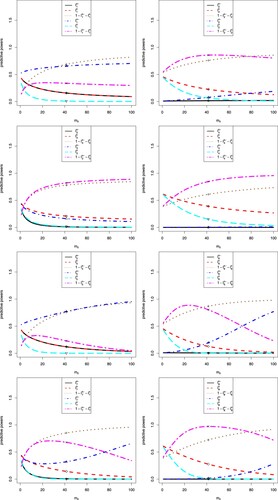
Table 4. The increase–decrease characteristics of $I_i^{s-}$, $I_i^s$, $1-I_i^{s-}-I_i^s$, $I_i^{o-}$, $I_i^o$ and $1-I_i^{o-}-I_i^o$ for $i=1,\dots ,8$ observed from Figure 3.

No.	$I_i^{s-}$	$I_i^s$	$1-I_i^{s-}-I_i^s$	$I_i^{o-}$	$I_i^o$	$1-I_i^{o-}-I_i^o$
1	↓	↓	↑	↑	↓	$\nearrow \searrow$
2	—	↓	↑	↑	↓	$\nearrow \searrow$
3	↓	↓	↑	↓	↓	↑
4	—	↓	↑	↑	↓	↑
5	↓	↓	↑	↑	↓	$\nearrow \searrow$
6	—	↓	↑	↑	↓	$\nearrow \searrow$
7	↓	↓	↑	$\searrow \nearrow$	↓	$\nearrow \searrow$
8	—	↓	↑	↑	↓	$\nearrow \searrow$

The sensitivity analysis of $d_1$ on the eight predictive powers is displayed in Figure 4. In the figure, we note the following issues.

• Note that $d_1$ is the observed treatment difference in the treatment group and the control (or placebo) group means of the interim data. The first and fifth predictive powers do not use the interim data, and thus they are missing in the figure.

• A negative $d_1$ favours tamoxifen, a positive $d_1$ favours control and a $d_1$ near 0 favours equivocal.

• From the figure, we see that $I_i^{s-}$ and $I_i^{o-}$ are decreasing functions of $d_1$, $I_i^s$ and $I_i^o$ are increasing functions of $d_1$, and $1-I_i^{s-}-I_i^s$ and $1-I_i^{o-}-I_i^o$ are first increasing and then decreasing functions of $d_1$, for i = 2, 3, 4, 6, 7, 8. The increase–decrease characteristics of $I_i^{s-}$, $I_i^{o-}$, $I_i^s$, $I_i^o$, $1-I_i^{s-}-I_i^s$ and $1-I_i^{o-}-I_i^o$ are compatible with the sign of $d_1$, for i = 2, 3, 4, 6, 7, 8, as a negative $d_1$ favours tamoxifen and $I_i^{s-}$ and $I_i^{o-}$ (the predictive powers for tamoxifen superior) have large values, a positive $d_1$ favours control and $I_i^s$ and $I_i^o$ (the predictive powers for control superior) have large values, and a $d_1$ near 0 favours equivocal and $1-I_i^{s-}-I_i^s$ and $1-I_i^{o-}-I_i^o$ (the predictive powers for equivocal) have large values.

• The optimistic prior favours tamoxifen, and thus $I_i^{o-}$ are consistently higher than $I_i^{s-}$, for i = 2, 3, 4, 6, 7, 8. Additionally, the sceptical prior favours control, and thus $I_i^s$ are consistently higher than $I_i^o$, for i = 2, 3, 4, 6, 7, 8.

• For the i-th (i = 2, 3, 4, 6, 7, 8) predictive power, there are six markers labelled °, △, +, ×, ⋄ and ▽, which correspond to $(d_1^r,I_i^{s-})$, $(d_1^r,I_i^{o-})$, $(d_1^r,E_i^s)$, $(d_1^r,E_i^o)$, $(d_1^r,I_i^s)$, and $(d_1^r,I_i^o)$, respectively. The predictive powers $(I_i^{s-},I_i^{o-},E_i^s,E_i^o,I_i^s,I_i^o)$ for i = 2, 3, 4, 6, 7, 8 in Table 3 are labelled in the figure by the six markers °, △, +, ×, ⋄ and ▽.

• In each plot, $1-I_i^{s-}-I_i^s$ and $1-I_i^{o-}-I_i^o$ are both bell shaped, with the latter being shifted right by a certain amount.

Figure 4. The sensitivity analysis of $d_1$ on the eight predictive powers.

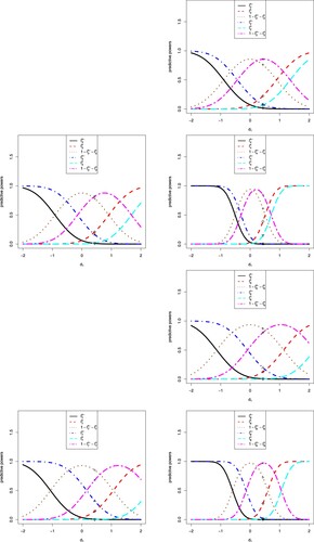
The sensitivity analysis of $m_1$ on the eight predictive powers are displayed in Figure 5. In the figure, we note the following issues.

• Note that $m_1$ is the per group number of patients of the interim data. The first and fifth predictive powers do not use the interim data, and thus they are missing in the figure.

• In each plot, s = 115 is fixed, $m_1=0,1,\dots ,s$, and $m_2=s-m_1=s,s-1,\dots ,0$.

• For the i-th (i = 2, 3, 4, 6, 7, 8) predictive power, there are six markers labelled °, △, +, ×, ⋄ and ▽, which correspond to $(m_1^r,I_i^{s-})$, $(m_1^r,I_i^{o-})$, $(m_1^r,E_i^s)$, $(m_1^r,E_i^o)$, $(m_1^r,I_i^s)$ and $(m_1^r,I_i^o)$, respectively. The predictive powers $(I_i^{s-},I_i^{o-},E_i^s,E_i^o,I_i^s,I_i^o)$ for i = 2, 3, 4, 6, 7, 8 in Table 3 are labelled in the figure by the six markers °, △, +, ×, ⋄ and ▽.

• Note that $\mathrm{V}\mathrm{a}\mathrm{r}\left(d_1|\delta \right)=2{\sigma }^2/m_1$, and thus when $m_1$ is large, the variance of $d_1|\delta$ will be small.

• When $m_1\to s=115$, the predictive powers tend to 1 or 0.

• The increase–decrease characteristics of $I_i^{s-}$, $I_i^s$, $1-I_i^{s-}-I_i^s$, $I_i^{o-}$, $I_i^o$ and $1-I_i^{o-}-I_i^o$ for i = 2, 3, 4, 6, 7, 8 observed from Figure 5 are summarized in Table 5. From the table, we observe that as $m_1$ increases, $I_i^{s-}$ decrease and $I_i^{o-}$ decrease for all eight predictive powers. $I_i^s$ are increasing and then decreasing functions of $m_1$ for the second and sixth predictive powers, and they are increasing functions of $m_1$ for the third, fourth, seventh and eighth predictive powers. $1-I_i^{s-}-I_i^s$ are increasing functions of $m_1$ for the second and sixth predictive powers, and they are increasing and then decreasing functions of $m_1$ for the third, fourth, seventh and eighth predictive powers. The $I_i^o$ is an increasing and then decreasing function of $m_1$ for the second predictive power, they are increasing functions of $m_1$ for the third and fourth predictive powers, and they are zero constants for the sixth, seventh and eighth predictive powers. $1-I_i^{o-}-I_i^o$ are increasing functions of $m_1$ for the second, sixth, seventh and eighth predictive powers, and they are increasing and then decreasing functions of $m_1$ for the third and fourth predictive powers.

Figure 5. The sensitivity analysis of $m_1$ on the eight predictive powers.

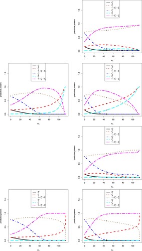
Table 5. The increase–decrease characteristics of $I_i^{s-}$, $I_i^s$, $1-I_i^{s-}-I_i^s$, $I_i^{o-}$, $I_i^o$ and $1-I_i^{o-}-I_i^o$ for i = 2, 3, 4, 6, 7, 8 observed from Figure 5.

No.	$I_i^{s-}$	$I_i^s$	$1-I_i^{s-}-I_i^s$	$I_i^{o-}$	$I_i^o$	$1-I_i^{o-}-I_i^o$
2	↓	$\nearrow \searrow$	↑	↓	$\nearrow \searrow$	↑
3	↓	↑	$\nearrow \searrow$	↓	↑	$\nearrow \searrow$
4	↓	↑	$\nearrow \searrow$	↓	↑	$\nearrow \searrow$
6	↓	$\nearrow \searrow$	↑	↓	—	↑
7	↓	↑	$\nearrow \searrow$	↓	—	↑
8	↓	↑	$\nearrow \searrow$	↓	—	↑

The sensitivity analysis of $m_2$ on the eight predictive powers is displayed in Figure 6. In the figure, we note the following issues.

• For the i-th ($i=1,\dots ,8$) predictive power, there are six markers labelled °, △, +, ×, ⋄ and ▽, which correspond to $(m_2^r,I_i^{s-})$, $(m_2^r,I_i^{o-})$, $(m_2^r,E_i^s)$, $(m_2^r,E_i^o)$, $(m_2^r,I_i^s)$ and $(m_2^r,I_i^o)$, respectively. The predictive powers $(I_i^{s-},I_i^{o-},E_i^s,E_i^o,I_i^s,I_i^o)$ for $i=1,\dots ,8$ in Table 3 are labelled in the figure by the six markers °, △, +, ×, ⋄ and ▽.

• Note that for the first and fifth predictive powers, the range of $m_2$ is $[50,200]$, and s = 115 for the real data is in this range, where $m_2$ is the whole sample size of the Phase III trial. For other predictive powers, the range of $m_2$ is $[0,s]=[0,115]$, $m_1=s-m_2$, and s = 115 is fixed, where $m_2$ is the per group number of patients of the future data after interim of the Phase III trial.

• Note that $\mathrm{V}\mathrm{a}\mathrm{r}\left(d_2|\delta \right)=2{\sigma }^2/m_2$, and thus when $m_2$ is large, the variance of $d_2|\delta$ will be small.

• The increase-decrease characteristics of $I_i^{s-}$, $I_i^s$, $1-I_i^{s-}-I_i^s$, $I_i^{o-}$, $I_i^o$ and $1-I_i^{o-}-I_i^o$ for $i=1,\dots ,8$ observed from Figure 6 are summarized in Table 6. From the table, we observe that as $m_2$ increases, $I_i^{s-}$ increase and $I_i^{o-}$ increase for all eight predictive powers. $I_i^s$ are increasing functions of $m_2$ for the first and fifth predictive powers, they are increasing and then decreasing functions of $m_2$ for the second and sixth predictive powers, and they are decreasing functions of $m_2$ for the third, fourth, seventh and eighth predictive powers. $1-I_i^{s-}-I_i^s$ are decreasing functions of $m_2$ for the first, second, fifth and sixth predictive powers, and they are increasing and then decreasing functions of $m_2$ for the third, fourth, seventh and eighth predictive powers. $I_i^o$ are zero constants for the first, fifth, sixth, seventh and eighth predictive powers, it is an increasing and then decreasing function of $m_2$ for the second predictive power, and they are decreasing functions of $m_2$ for the third and fourth predictive powers. $1-I_i^{o-}-I_i^o$ are decreasing functions of $m_2$ for the first, second, fifth, sixth, seventh and eighth predictive powers, and they are increasing and then decreasing functions of $m_2$ for the third and fourth predictive powers. Note that some predictive powers display the same increase–decrease characteristics, and they are the first and fifth predictive powers, the third and fourth predictive powers, and the seventh and eighth predictive powers.

Figure 6. The sensitivity analysis of $m_2$ on the eight predictive powers.

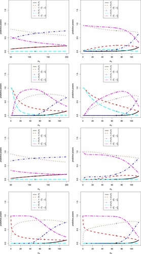
Table 6. The increase–decrease characteristics of $I_i^{s-}$, $I_i^s$, $1-I_i^{s-}-I_i^s$, $I_i^{o-}$, $I_i^o$ and $1-I_i^{o-}-I_i^o$ for $i=1,\dots ,8$ observed from Figure 6.

No.	$I_i^{s-}$	$I_i^s$	$1-I_i^{s-}-I_i^s$	$I_i^{o-}$	$I_i^o$	$1-I_i^{o-}-I_i^o$
1	↑	↑	↓	↑	—	↓
2	↑	$\nearrow \searrow$	↓	↑	$\nearrow \searrow$	↓
3	↑	↓	$\nearrow \searrow$	↑	↓	$\nearrow \searrow$
4	↑	↓	$\nearrow \searrow$	↑	↓	$\nearrow \searrow$
5	↑	↑	↓	↑	—	↓
6	↑	$\nearrow \searrow$	↓	↑	—	↓
7	↑	↓	$\nearrow \searrow$	↑	—	↓
8	↑	↓	$\nearrow \searrow$	↑	—	↓

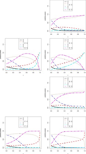
The sensitivity analysis of t on the eight predictive powers are displayed in Figure 7. In the figure, we note the following issues.

• Note that t is the information time of the interim data. The first and fifth predictive powers do not use the interim data, and thus they are missing in the figure.

• Figures 5 and 7 are the same with the only differences of the x-labels and x-ranges, which are $(m_1,[0,115\left]\right)$ and $(t,[0,1\left]\right)$, respectively. Note that $m_1=0,1,\dots ,s=115$and $t=\frac{m_1}{m_1+m_2}=\frac{m_1}{s}\in [0,1].$

• For the i-th (i = 2, 3, 4, 6, 7, 8) predictive power, there are six markers labelled °, △, +, ×, ⋄, and ▽, which correspond to $(t^r,I_i^{s-})$, $(t^r,I_i^{o-})$, $(t^r,E_i^s)$, $(t^r,E_i^o)$, $(t^r,I_i^s)$ and $(t^r,I_i^o)$, respectively. The predictive powers $(I_i^{s-},I_i^{o-},E_i^s,E_i^o,I_i^s,I_i^o)$ for i = 2, 3, 4, 6, 7, 8 in Table 3 are labelled in the figure by the six markers °, △, +, ×, ⋄ and ▽.

• When $t\to 1$, the predictive powers tend to 1 or 0.

• The increase–decrease characteristics of $I_i^{s-}$, $I_i^s$, $1-I_i^{s-}-I_i^s$, $I_i^{o-}$, $I_i^o$ and $1-I_i^{o-}-I_i^o$ for i = 2, 3, 4, 6, 7, 8 observed from Figure 7 are the same as those observed from Figure 5, which are summarized in Table 5.

Figure 7. The sensitivity analysis of t on the eight predictive powers.

5. Conclusion and discussion

For the randomized controlled early phase and Phase III trials, suppose that the model and the prior are given by (3(3) $\begin{array}{rl}& d_1|\delta \sim N(\delta ,\frac{2{\sigma }^2}{m_1}),d_2|\delta \sim N(\delta ,\frac{2{\sigma }^2}{m_2}),\\ & \times \delta |d_0\sim N(d_0,\frac{2{\sigma }^2}{m_0}).\end{array}$(3) ). We provide two tables in this article. The eight predictive powers with historical and interim data, their analytical expressions, the predictive distributions, the data used, and the references for the hypotheses $H_0:\delta \le {\delta }_0$ versus $H_1:\delta >{\delta }_0$ are given in Table 1. The eight predictive powers with historical and interim data, their analytical expressions, the predictive distributions and the data used for the reversed hypotheses $H_0:\delta \ge {\delta }_0$ versus $H_1:\delta <{\delta }_0$ are given in Table 2. Moreover, the data structures of the historical data, interim data and future data are described in Figure 1. Furthermore, the eight predictive powers with historical and interim data for the hypotheses and the reversed hypotheses are utilized to guide the futility analysis in the tamoxifen example. Finally, extensive simulations are conducted to investigate the sensitivity analysis of priors ($d_0$), sample sizes ($m_0$, $m_1$, $m_2$), interim result ($d_1$) and interim time (t) on the eight predictive powers.

In addition to the four predictive powers ($I_1$, $I_4$, $I_5$, $I_8$) summarized in Table 1, we discover and calculate another four predictive powers ($I_2$, $I_3$, $I_6$, $I_7$) also summarized in Table 1, for the hypotheses $H_0:\delta \le {\delta }_0$ versus $H_1:\delta >{\delta }_0$. Moreover, we calculate eight predictive powers ($I_1^{-}$ to $I_8^{-}$) summarized in Table 2, for the reversed hypotheses $H_0:\delta \ge {\delta }_0$ versus $H_1:\delta <{\delta }_0$. The combination of Tables 1 and 2 gives us a complete picture of the predictive powers with historical and interim data for futility and efficacy analysis, as illustrated in Table 3.

By comparing these eight predictive power calculations, one main difference among them is how many times the historical data and interim data are utilized. For example, the historical data and the interim data could be used once or twice in these calculations. It may be confusing to the reader why the historical data or interim data could be used twice. For example, if the predictive power is calculated at the time when the required interim data are collected, why the authors incorporate the interim data into the prior specification given the interim data have been contributed to the likelihood? These are the fourth and eighth predictive powers in Tables 1 and 2. Note that in Table 1, the fourth predictive power is (6.15) in Spiegelhalter et al. (2004), and it is the average classical conditional power with respect to the updated new prior $\pi (\delta |d_0,d_1)$; the eighth predictive power is (6.18) in Spiegelhalter et al. (2004), and it is the average Bayesian conditional power with respect to the updated new prior $\pi (\delta |d_0,d_1)$. If one is willing to use the historical data and interim data only once, then one could use the second and third predictive powers in the two tables, and the two predictive powers are discovered by us. Another possible solution to use the data twice is to use the external data.

Two sets of one-sided hypotheses are considered throughout the paper, and they are both needed. That is, both Tables 1 and 2 are needed. As discussed in the real data example, for $j=1,\dots ,8$, the j-th predictive power $I_j$ (see Table 1) is for control superior, the j-th predictive power $I_j^{-}$ (see Table 2) is for tamoxifen superior, and $1-I_j-I_j^{-}$ is for equivocal.

We have assumed a known variance (${\sigma }^2$), which is unrealistic. However, in the literature and real applications (see for instance Chuang-Stein, 2006; Kirby et al., 2012; Lan & Wittes, 2012; O'Hagan et al., 2005; Spiegelhalter et al., 2004; Wang et al., 2006), it is common practice to assume that the variance ${\sigma }^2$ is known to obtain analytical solutions, such as $\mathrm{\Phi }(\cdot )$ for powers and average powers. When the variance is unknown, one might use the historical data to specify a sampling prior for ${\sigma }^2$ (Chen et al., 2011). Alternatively, one might utilize a t statistic. As stated in O'Hagan et al. (2005), the sampling distribution of t is a non-central t distribution (which only becomes an ordinary Student t distribution if $\delta =0$). Nevertheless, based on previous Phase II trials or publications, the estimate of ${\sigma }^2$ is good enough, such that it provides some assurance to the practitioners that probably there is no need to have a prior for ${\sigma }^2$ when designing the Phase III trial. Furthermore, in practice and in publications, it is not common to add a prior to ${\sigma }^2$ in the calculations in frequentist framework and mixed frequentist and Bayesian framework. However, it is very common to include prior on ${\sigma }^2$ in pure Bayesian framework.

We have assumed equal variances for the normally distributed responses of two treatments of the Phase III trial. The equal variances assumption can be reasonably met in reality by exploiting the randomized controlled Phase III trial. This statement needs to be further justified. Consider a well-designed (patient-masked and outcome observer-blinded) placebo controlled trial where patients in the control group will demonstrate (approximately) the same outcome before and after treatment exposure. If the study drug is effective in a certain portion of patients in the treatment arm, the outcome for these patients will be different (shifted by a certain magnitude) before and after treatment. Hence, the variance in the treatment arm is expected to be higher than that in the control arm, unless the study drug is similarly effective in every patient who received it. On the other hand, if the study drug leads to an elevation (or decrease) of the outcome to a certain boundary value, the variance in the treatment group may be even smaller than that in the control group. Therefore, for simplicity, we assume equal variances for the normally distributed responses of two treatments. However, it is not uncommon to assume unequal variances in pure Bayesian framework.

The method demonstrated in Section 2 assumes the treatment arms have the same randomization ratio for illustration purpose, but the method can be easily adapted when the randomization ratios are not balanced. See the Conclusions and Discussion section in Deng et al. (2020) for details.

For simplicity, we assume that outcome measurements are available for all individuals in the study and that everyone in the treatment arm and the control arm is fully adherent to the treatment they are allocated to, i.e., no non-compliance or treatment arm cross-over. In other words, the meaning of the effect parameter we are going to identify from the observed data is the true average treatment effect.

For simplicity, we have assumed the true treatment effects based on the historical data of the early phase trial, the interim data, and the future data of the Phase III trial are the same. This assumption has also been used in the literature. For example, Chuang-Stein (2006) has assumed that the true treatment effects based on the Phase II trial and the Phase III trial are the same. Spiegelhalter et al. (2004) have assumed that the true treatment effects based on the interim data and the future data of the Phase III trial are the same.

The analytical derivations in Section 2 are based on normal likelihoods. As explained in Section 2.4 of Spiegelhalter et al. (2004), normal likelihoods can be used for binary data, survival data, count responses and continuous responses. In the real data example, we use a data example where survival data (disease-free survival time) is the primary outcome variable. Note that, in general, effect estimates such as log hazard ratios follow a normal distribution. It is important to stress that $m_0$, $m_1$ and $m_2$ do represent number of events and are not sample sizes in this context.

Intuitively, when the historical and interim data are available, they should be used to give a more accurate prediction, as the predictive powers shown in Table 3. Therefore, we recommend reporting all eight predictive powers in practice to have a complete picture for futility and efficacy analysis.

If one is interested in evaluating whether the incorporation of the historical data or interim data can improve the estimation of treatment effects for futility analysis, a real data example is not enough. One may need to conduct simulation studies to evaluate estimation accuracy or correct stopping rates by using the historical data (or interim data) or not. Alternatively, one may use the Receiver Operating Characteristic (ROC) curve as a tool to evaluate and compare operating characteristics by using the historical data (or interim data) or not. In fact, we are currently working on the analytical ROC analyses of the eight predictive powers, and the elaborated version deserves another publication.

Table 3 summarizes the predictive power values for the example data under three predefined scenarios (tamoxifen superior, equivocal, and control superior) considering sceptical and optimistic priors. Note that the three scenarios are based on the notion of ‘statistical significance’, i.e. if 0 is included in the $95\mathrm{\%}$ posterior interval for the target parameter δ or not. One could consider the specification of these scenarios as to consider clinically relevant equivalence margins for δ (say $\pm 5\mathrm{\%}$ or $\pm 10\mathrm{\%}$). The statement ‘equivocal’ would then only hold, if both credible interval limits fall within these margins.

The way the results are presented right now suggests to stop the trial for futility but this may in fact be an imprecision issue due to small $m_2$ (or limited overall number of events). This claim is supported by the fact that even for very low optimistic predictive power values under scenario ‘Tamoxifen superior’, the sceptical predictive power values under scenario ‘Control superior’ remain relatively low. This means that the confidence intervals or credible intervals of δ often are too wide to exclude 0 for the target parameter δ. The lengths of the confidence intervals or credible intervals of δ and the lengths of the intervals of $d_2$ of equivocal are decreasing functions of $m_2$. That is, when $m_2$ is small (imprecision), the lengths of the intervals of $d_2$ of equivocal are large. Hence, it is probably that the probabilities of equivocal for the powers and predictive powers will be large. It is worth noting that the imprecision issues due to small $m_2$ (or limited overall number of events) are related to all four powers (CP, CCP, BP and BCP) and all eight predictive powers. We are currently working on the imprecision issue, and the elaborated version deserves another publication.

Assuming a flat prior with infinite tales ($\pi \left(\delta \right)\propto 1$) seems overly conservative, the uniform prior interval would in practice rather be $[a,b]$ with $\left|b\right|>\left|a\right|$ and $a\le 0<b$ for the hypotheses $H_0:\delta \le 0$ versus $H_1:\delta >0$, expressing the optimism of the drug-developer as the drug made it already beyond lab and animal testing. That is, it is useful to allow for the incorporation of a proper uniform prior for δ when estimating the posterior $\delta |d_0$, into formula (3(3) $\begin{array}{rl}& d_1|\delta \sim N(\delta ,\frac{2{\sigma }^2}{m_1}),d_2|\delta \sim N(\delta ,\frac{2{\sigma }^2}{m_2}),\\ & \times \delta |d_0\sim N(d_0,\frac{2{\sigma }^2}{m_0}).\end{array}$(3) ) and following expressions. However, in this situation, one may not obtain analytical solutions. Then one should be able to derive the predictive powers numerically.

Acknowledgments

The authors are extremely grateful to the editor, the associate editor, and the reviewer for their insightful comments that led to significant improvement of the article.

Disclosure statement

No potential conflict of interest was reported by the authors.

Additional information

Funding

The research was supported by National Social Science Fund of China [grant number 21XTJ001].

References

- Chen, M. H., Ibrahim, J. G., Lam, P., Yu, A., & Zhang, Y. Y. (2011). Bayesian design of noninferiority trials for medical devices using historical data. Biometrics, 67(3), 1163–1170. https://doi.org/10.1111/biom.2011.67.issue-3
- Choi, S. C., Smith, P. J., & Becker, D. P. (1985). Early decision in clinical trials when the treatment differences are small. Controlled Clinical Trials, 6(4), 280–288. https://doi.org/10.1016/0197-2456(85)90104-7
- Chuang-Stein, C. (2006). Sample size and the probability of a successful trial. Pharmaceutical Statistics, 5(4), 305–309. https://doi.org/10.1002/(ISSN)1539-1612
- Chuang-Stein, C., & Kirby, S. (2017). Quantitative decisions in drug development. Springer.
- Deng, Q. Q., Zhang, Y. Y., Roy, D., & Chen, M. H. (2020). Superiority of combining two independent trials in interim futility analysis. Statistical Methods in Medical Research, 29(2), 522–540. https://doi.org/10.1177/0962280219840383
- Dignam, J. J., Bryant, J., Wieand, H. S., Fisher, B., & Wolmark, N. (1998). Early stopping of a clinical trial when there is evidence of no treatment benefit: protocol b-14 of the national surgical adjuvant breast and bowel project. Controlled Clinical Trials, 19(6), 575–588. https://doi.org/10.1016/S0197-2456(98)00041-5
- Dmitrienko, A., & Wang, M. D. (2006). Bayesian predictive approach to interim monitoring in clinical trials. Statistics in Medicine, 25(13), 2178–2195. https://doi.org/10.1002/(ISSN)1097-0258
- Ibrahim, J. G., Chen, M. H., Lakshminarayanan, M., Liu, G. F., & Heyse, J. F. (2015). Bayesian probability of success for clinical trials using historical data. Statistics in Medicine, 34(2), 249–264. https://doi.org/10.1002/sim.v34.2
- Jiang, K. (2011). Optimal sample sizes and go/no-go decisions for phase ii/iii development programs based on probability of success. Statistics in Biopharmaceutical Research, 3(3), 463–475. https://doi.org/10.1198/sbr.2011.10068
- Kirby, S., Burke, J., Chuang-Stein, C., & Sin, C. (2012). Discounting phase 2 results when planning phase 3 clinical trials. Pharmaceutical Statistics, 11(5), 373–385. https://doi.org/10.1002/pst.1521
- Lan, K. K. G., & Wittes, J. T. (2012). Some thoughts on sample size: a Bayesian frequentist hybrid approach. Clinical Trials, 9(5), 561–569. https://doi.org/10.1177/1740774512453784
- O'Hagan, A., Stevens, J. W., & Campbell, M. J. (2005). Assurance in clinical trial design. Pharmaceutical Statistics, 4(3), 187–201. https://doi.org/10.1002/(ISSN)1539-1612
- Schmidli, H., Bretz, F., & Racine-Poon, A. (2007). Bayesian predictive power for interim adaptation in seamless phase ii/iii trials where the endpoint is survival up to some specified timepoint. Statistics in Medicine, 26(27), 4925–4938. https://doi.org/10.1002/(ISSN)1097-0258
- Spiegelhalter, D. J., Abrams, K. R., & Myles, J. P. (2004). Bayesian approaches to clinical trials and health-care evaluation. Wiley.
- Spiegelhalter, D. J., Freedman, L. S., & Blackburn, P. R. (1986). Monitoring clinical trials: conditional or predictive power?. Controlled Clinical Trials, 7(1), 8–17. https://doi.org/10.1016/0197-2456(86)90003-6
- Trzaskoma, B., & Sashegyi, A. (2007). Predictive probability of success and the assessment of futility in large outcomes trials. Journal of Biopharmaceutical Statistics, 17(1), 45–63. https://doi.org/10.1080/10543400601001485
- Tsiatis, A. A. (1981). The asymptotic joint distribution of the efficient scores test for the proportional hazards model calculated over time. Biometrika, 68(1), 311–315. https://doi.org/10.1093/biomet/68.1.311
- Wang, S. J., Hung, H. M. J., & O'Neill, R. T. (2006). Adapting the sample size planning of a phase iii trial based on phase ii data. Pharmaceutical Statistics, 5(2), 85–97. https://doi.org/10.1002/(ISSN)1539-1612
- Zhang, J., Carlin, B. P., Neaton, J. D., Soon, G. G., Nie, L., Kane, R., Virnig, B. A., & Chu, H. (2014). Network meta-analysis of randomized clinical trials: reporting the proper summaries. Clinical Trials, 11(2), 246–262. https://doi.org/10.1177/1740774513498322
- Zhang, Y. Y., Rong, T. Z., & Li, M. M. (2020a). The contemplated average success probability for normally distributed models with an application to optimal sample sizes selection. Statistics in Medicine, 39(23), 3173–3183. https://doi.org/10.1002/sim.v39.23
- Zhang, Y. Y., Rong, T. Z., & Li, M. M. (2020b). A new expectation identity and its application in the calculations of predictive powers assuming normality. Chinese Journal of Applied Probability and Statistics, 36(5), 523–535. https://doi.org/10.3969/j.issn.1001-4268.2020.05.007
- Zhang, Y. Y., & Ting, N. (2018). Bayesian sample size determination for a phase iii clinical trial with diluted treatment effect. Journal of Biopharmaceutical Statistics, 28(6), 1119–1142. https://doi.org/10.1080/10543406.2018.1436556
- Zhang, Y. Y., & Ting, N. (2020). Sample size considerations for a phase iii clinical trial with diluted treatment effect. Statistics in Biopharmaceutical Research, 12(3), 311–321. https://doi.org/10.1080/19466315.2019.1599414