A new result on recovery sparse signals using orthogonal matching pursuit

Abstract

Orthogonal matching pursuit (OMP) algorithm is a classical greedy algorithm widely used in compressed sensing. In this paper, by exploiting the Wielandt inequality and some properties of orthogonal projection matrix, we obtained a new number of iterations required for the OMP algorithm to perform exact recovery of sparse signals, which improves significantly upon the latest results as we know.

Keywords:

• Compressed sensing
• orthogonal matching pursuit
• Wielandt inequality
• orthogonal projection matrix

1. Introduction

Orthogonal matching pursuit (OMP) has received growing attention due to its simplicity and competitive reconstruction performance recently. Consider the following compressed linear model: (1) $y=\mathrm{\Phi }x,$(1) where $x\in {\mathbf{C}}^n$ is a K-sparse signal (i.e., $\Vert x{\Vert }_0\le K$), $\mathrm{\Phi }=[{\varphi }_1,{\varphi }_2,\dots ,{\varphi }_n]\in {\mathbf{C}}^{m\times n}$ is a known measurement matrix with $m\ll n$ and $y\in {\mathbf{C}}^m$ is the observation signal. It has been demonstrated that under some appropriate conditions on Φ, OMP can reliably recover the signal x based on a set of compressive observations y by iteratively identifying the support of the sparse signal according to the maximum correlation between columns of measurement matrix and the current residual. See Table 1 for a detailed description of the OMP algorithm (Cai & Wang, 2011; Chang & Wu, 2014; Tropp & Gilbert, 2007; Wang & Shim, 2016; Wen et al., 2020, 2017; Wu et al., 2013). In Table 1, $supp\left(x\right)$ is the set of nonzero positions in x. $r^k$ denotes the residual after the kth iteration of OMP and $T^k$ the estimated support set within kth iteration of OMP.

Table 1. Orthogonal matching pursuit.

Input:	$\mathrm{\Phi },y$, and maximum iteration number $k_{max}$
Initialize:	$k=0,r^0=y,T^0=\mathrm{\varnothing }$
while	$k<k_{max}$, do
	k = k + 1,
	$t^k=\arg \underset{1\le i\le n}{max}|〈r^{k-1},{\varphi }_i〉|,$
	$T^k=T^{k-1}\cup \left\{t^k\right\},$
	${\hat{x}}^k=\arg \underset{u\in {\mathbb{C}}^n:\mathrm{s}\mathrm{u}\mathrm{p}\mathrm{p}\left(u\right)\subset T^k}{min}\Vert y-\mathrm{\Phi }u{\Vert }_2,$
	$r^k=y-\mathrm{\Phi }{\hat{x}}^k.$
Output:	$T^k$ and ${\hat{x}}^k$

In compressed sensing, a commonly used framework for analysing the recovery performance is the restricted isometry property (RIP) (Cai et al., 2010; Candes & Tao, 2005; Chang & Wu, 2014). A matrix Φ is said to satisfy the RIP of order K if there exists a constant $\delta \in [0,1)$ such that (2) $(1-\delta )\Vert x{\Vert }_2^2\le \Vert \mathrm{\Phi }x{\Vert }_2^2\le (1+\delta )\Vert x{\Vert }_2^2,$(2) for all K-sparse signal x. In particular, the minimum of all constants δ satisfying (2(2) $(1-\delta )\Vert x{\Vert }_2^2\le \Vert \mathrm{\Phi }x{\Vert }_2^2\le (1+\delta )\Vert x{\Vert }_2^2,$(2) ) is called the K-order Restricted Isometry Constant (RIC) and denoted by ${\delta }_K$. Over the years, many RIP-based conditions have been proposed to guarantee exact recovery of any K-sparse signals via OMP in K iterations. It has been shown in Davenport and Wakin (2010) that ${\delta }_{K+1}<(3\sqrt{K}{)}^{-1}$ is sufficient for OMP to recover any K-sparse signals x in K iterations. The sufficient reconstruction condition of OMP is then improved to ${\delta }_{K+1}<(1+2\sqrt{K}{)}^{-1}$ by Huang and Zhu (2011). Mo (2015) demonstrated that ${\delta }_{K+1}<(\sqrt{K+1}{)}^{-1}$ is a sharp condition for exact recovery of any K-sparse signal with OMP in K iterations. Our recent work Liu et al. (2017) provides some sufficient conditions for recovering restricted classes of K-sparse signals with a more relaxed bound on RIC.

Obviously, running fewer number of iterations of OMP offers many benefits and many efforts have been made to improve the condition (Cai et al., 2009; Chang & Wu, 2014; Li & Wen, 2019; Wen et al., 2017; Wu et al., 2013). In Livshitz (2012), Livshitz showed that with proper choices of α and β ($\alpha \sim 2\times {10}^5,\text{β}\sim {10}^{-6}$), OMP accurately reconstructs K-sparse signals in $\alpha K^{1.2}$ iterations under ${\delta }_{\alpha K^{1.2}}=\text{β}{K}^{-0.2}$. It has been shown by Zhang (2011) that OMP recovers any K-sparse signal in $30\mathrm{K}$ iterations under ${\delta }_{31K}\le 3^{-1}$. Livshitz and Temlyakov (2014) considered random sparse signals and showed that with high probability, these signals can be recovered within $\lceil (1+ϵ)K\rceil$ iterations of OMP for any $ϵ>0$. Recently, Wang and Shim (2016) showed that if (3) $c\ge -\frac{4(1+\delta )}{1-\delta }\ln (\frac{1}{2}-\sqrt{\frac{\delta }{2+2\delta }}),$(3) and ${\delta }_{\left[\right(c+1\left)K\right]}\le \delta$, OMP can recover the K-sparse signals in $\lceil cK\rceil$ iterations. It is the best result as we know in the literature.

In this paper, we present a new result on how many iterations of OMP would be enough to guarantee exact recovery of sparse signals: $c\ge -\frac{4(1+{\delta }_1)}{1-\delta }\ln \left(\frac{1-\delta }{2}\right),$ which improves significantly upon the results proposed in Wang and Shim (2016).

We first give some notation. Let $\mathbf{N}=\{0,1,2,\dots \},{\mathbf{N}}^{+}=\{1,2,\dots \}$ and ${\mathrm{\Omega }}_n=\{1,2,\dots ,n\}$. $[\cdot ]$ and $\lceil \cdot \rceil$ denote floor and ceiling function, respectively. For any two sets Λ and Γ, let $\mathrm{\Lambda }\setminus \mathrm{\Gamma }=\{i:i\in \mathrm{\Lambda },i\notin \mathrm{\Gamma }\}$, and $\left|\mathrm{\Lambda }\right|$ is the cardinality of Λ. For $\mathrm{\Lambda }\subset {\mathrm{\Omega }}_n$ and $\mathrm{\Lambda }\ne \mathrm{\varnothing }$, ${\mathrm{\Phi }}_{\mathrm{\Lambda }}$ denotes the submatrix of Φ that contains only the columns indexed by Λ and $x_{\mathrm{\Lambda }}$ denotes the subvector of x that contains only the entries indexed by Λ, and $\mathrm{s}\mathrm{p}\mathrm{a}\mathrm{n}\left({\mathrm{\Phi }}_{\mathrm{\Lambda }}\right)$ represents the span of columns in ${\mathrm{\Phi }}_{\mathrm{\Lambda }}$. Let $P_{\mathrm{\Lambda }}={\mathrm{\Phi }}_{\mathrm{\Lambda }}({\mathrm{\Phi }}_{\mathrm{\Lambda }}^{\ast }{\mathrm{\Phi }}_{\mathrm{\Lambda }}{)}^{+}{\mathrm{\Phi }}_{\mathrm{\Lambda }}^{\ast }$ stand for an orthogonal projection matrix onto $\mathrm{s}\mathrm{p}\mathrm{a}\mathrm{n}\left({\mathrm{\Phi }}_{\mathrm{\Lambda }}\right)$, where ${\mathrm{\Phi }}^{\ast }$ is the conjugate transpose of the matrix Φ, and $({\mathrm{\Phi }}_{\mathrm{\Lambda }}^{\ast }{\mathrm{\Phi }}_{\mathrm{\Lambda }}{)}^{+}$ is Moore–Penrose pseudo inverse of ${\mathrm{\Phi }}_{\mathrm{\Lambda }}^{\ast }{\mathrm{\Phi }}_{\mathrm{\Lambda }}$. $P_{\mathrm{\Lambda }}^{\mathrm{\perp }}=I_m-P_{\mathrm{\Lambda }}$ is an orthogonal projection matrix onto the orthogonal complement of $\mathrm{s}\mathrm{p}\mathrm{a}\mathrm{n}\left({\mathrm{\Phi }}_{\mathrm{\Lambda }}\right)$, where $I_m$ denotes the identity matrix. In particular, if $\mathrm{\Lambda }=\mathrm{\varnothing }$, then $x_{\mathrm{\varnothing }}$ is a 0-by-1 empty vector, ${\mathrm{\Phi }}_{\mathrm{\varnothing }}$ is an m-by-0 empty matrix, ${\mathrm{\Phi }}_{\mathrm{\varnothing }}{x}_{\mathrm{\varnothing }}$ is an m-by-1 zero matrix and $\mathrm{s}\mathrm{p}\mathrm{a}\mathrm{n}\left({\mathrm{\Phi }}_{\mathrm{\varnothing }}\right):=\left\{0\right\}$. For further details on empty matrices, see, e.g., Bernstein (2005).

2. Main results

For notational simplicity, we denote ${\mathrm{\Gamma }}^k=T\setminus T^k$.

Theorem 2.1

For any $\delta \in (0,1)$, let $\alpha =-\frac{4(1+{\delta }_1)}{1-\delta }\ln \left(\frac{1-\delta }{2}\right),$ and $\kappa =\left[\alpha K\right]$. If the measurement matrix Φ in (1(1) $y=\mathrm{\Phi }x,$(1) ) satisfies the RIP of order $K+\kappa$ and ${\delta }_{K+\kappa }\le \delta ,$ then $\left|{\mathrm{\Gamma }}^{\kappa }\right|=0$.

Remark 2.1

Performance of Theorem 2.1

From Theorem 2.1, if (4) $c\ge -\frac{4(1+{\delta }_1)}{1-\delta }\ln \left(\frac{1-\delta }{2}\right),$(4) and ${\delta }_{\left[\right(c+1\left)K\right]}\le \delta$, then OMP perfectly recovers the signal x from the measurements $y=\mathrm{\Phi }x$ in $\left[cK\right]$ iteration. In the following, we compare the lower bound in (4(4) $c\ge -\frac{4(1+{\delta }_1)}{1-\delta }\ln \left(\frac{1-\delta }{2}\right),$(4) ) with the result of Wang and Shim (2016), which has been showed in (3(3) $c\ge -\frac{4(1+\delta )}{1-\delta }\ln (\frac{1}{2}-\sqrt{\frac{\delta }{2+2\delta }}),$(3) ). We first establish an upper bound for the ratio of (4(4) $c\ge -\frac{4(1+{\delta }_1)}{1-\delta }\ln \left(\frac{1-\delta }{2}\right),$(4) ) to (3(3) $c\ge -\frac{4(1+\delta )}{1-\delta }\ln (\frac{1}{2}-\sqrt{\frac{\delta }{2+2\delta }}),$(3) ) by using monotonicity property of the RIC (${\delta }_1\le {\delta }_{K+\kappa }$) as $R\left(\delta \right):=\frac{\ln \left(\frac{1-\delta }{2}\right)}{\ln (\frac{1}{2}-\sqrt{\frac{\delta }{2+2\delta }})}.$ It is easy to check that $R\left(\delta \right)<1$ for $0<\delta <1$, 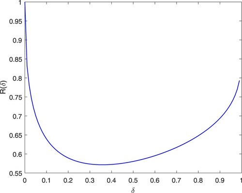which means the lower bound of c in this paper is uniformly smaller than the one proposed in Wang and Shim (2016). See Figure 1, for example, we have $R\left(3^{-1}\right)=0.57$ and $R\left(2^{-1}\right)=0.58$. For $0.015<\delta <0.993$, we have $0.57<R\left(\delta \right)<0.8$. That is, nearly 98% of the values of the bounds proposed in this paper is less than 0.8 times of the one in (3(3) $c\ge -\frac{4(1+\delta )}{1-\delta }\ln (\frac{1}{2}-\sqrt{\frac{\delta }{2+2\delta }}),$(3) ).

Figure 1. Performance of Theorem 2.1.

Remark 2.2

Main differences with the previous work

Our methods have several key distinctions in construction of the more efficient lower and upper bounds of resident in OMP. First, Wang and Shim (2016) obtained the upper bound of residual in OMP algorithm based on the following fundamental set: $\{\Vert x_{\mathrm{\Gamma }}{\Vert }_2:\mathrm{\Gamma }\subset {\mathrm{\Gamma }}^k\}.$ We modified the above set to $\{\Vert {\mathrm{\Phi }}_{\mathrm{\Gamma }}{x}_{\mathrm{\Gamma }}{\Vert }_2:\mathrm{\Gamma }\subset {\mathrm{\Gamma }}^k\},$ which leads to a more efficient upper bound of resident in OMP algorithm (see inequality (17(17) $\Vert r^{n_1}{\Vert }_2^2<(1-{\delta }^2)\Vert {\mathrm{\Phi }}_{{\mathrm{\Gamma }}_k\setminus {\mathrm{\Gamma }}_{L\left(k\right)}^k}{x}_{{\mathrm{\Gamma }}_k\setminus {\mathrm{\Gamma }}_{L\left(k\right)}^k}{\Vert }_2^2.$(17) ) of Section 3.3). Second, Livshitz and Temlyakov (2014), Wang and Shim (2016), and Zhang (2011) only use RIP to obtain the lower bound of resident. However, in this paper, we not only used RIP, but also utilized the Wielandt inequality (Wang & Ip, 1999) to derive more efficient lower bound of resident (see inequality (16(16) $\Vert r^{n_1}{\Vert }_2^2\ge (1-{\delta }^2)\Vert {\mathrm{\Phi }}_{{\mathrm{\Gamma }}^{n_1}}{x}_{{\mathrm{\Gamma }}^{n_1}}{\Vert }_2^2.$(16) ) of Section 3.3). The details can be found in the following sections.

3. Proof of the main theorem

3.1. Preliminaries

In the following, we introduce the subset ${\mathrm{\Gamma }}_{\tau }^k$ of ${\mathrm{\Gamma }}^k$ based on the magnitude of elements in the set $\{\Vert {\mathrm{\Phi }}_{\mathrm{\Gamma }}{x}_{\mathrm{\Gamma }}{\Vert }_2:\mathrm{\Gamma }\subset {\mathrm{\Gamma }}^k\}$. For $k,\tau \in N$ and ${\mathrm{\Gamma }}^k\ne \mathrm{\varnothing }$, let (5) $\begin{array}{rl}& {\mathrm{\aleph }}_{\tau }=\{\mathrm{\Lambda }:\mathrm{\Lambda }\subset {\mathrm{\Gamma }}^k,|\mathrm{\Lambda }|\le 2^{\tau }-1\},\end{array}$(5) (6) $\begin{array}{rl}& f\left(\tau \right)=min\{\Vert {\mathrm{\Phi }}_{{\mathrm{\Gamma }}^k\setminus \mathrm{\Lambda }}{x}_{{\mathrm{\Gamma }}^k\setminus \mathrm{\Lambda }}\Vert :\mathrm{\Lambda }\in {\mathrm{\aleph }}_{\tau }\}.\end{array}$(6) It is clear that ${\mathrm{\aleph }}_{\tau }\subset {\mathrm{\aleph }}_{\tau +1},$ and $f\left(\tau \right)\ge f(\tau +1)$ with $\tau \in \mathbf{N}$.

Definition 3.1

If subset ${\mathrm{\Gamma }}_{\tau }^k$ in ${\mathrm{\aleph }}_{\tau }$ satisfies: (a) $\Vert {\mathrm{\Phi }}_{{\mathrm{\Gamma }}^k\setminus {\mathrm{\Gamma }}_{\tau }^k}{x}_{{\mathrm{\Gamma }}^k\setminus {\mathrm{\Gamma }}_{\tau }^k}{\Vert }_2=f\left(\tau \right)$ and (b) $\left|{\mathrm{\Gamma }}_{\tau }^k\right|=max\left\{\right|\mathrm{\Lambda }|:\mathrm{\Lambda }\in {\mathrm{\aleph }}_{\tau },\Vert {\mathrm{\Phi }}_{{\mathrm{\Gamma }}^k\setminus \mathrm{\Lambda }}{x}_{{\mathrm{\Gamma }}^k\setminus \mathrm{\Lambda }}{\Vert }_2=f(\tau \left)\right\}$, then ${\mathrm{\Gamma }}_{\tau }^k$ is said to be the $\mathrm{\Phi }-k-\tau$ characteristic set of x.

It is easy to verify that the characteristic set ${\mathrm{\Gamma }}_{\tau }^k$ has the following properties:

1. $\left|{\mathrm{\Gamma }}_{\tau }^k\right|\le 2^{\tau }-1$, for $\tau \in \mathbf{N}$;

2. If $\mathrm{\Gamma }\subset {\mathrm{\Gamma }}^k$ and $\Vert {\mathrm{\Phi }}_{\mathrm{\Gamma }}{x}_{\mathrm{\Gamma }}{\Vert }_2<\Vert {\mathrm{\Phi }}_{{\mathrm{\Gamma }}^k\setminus {\mathrm{\Gamma }}_{\tau }^k}{x}_{{\mathrm{\Gamma }}^k\setminus {\mathrm{\Gamma }}_{\tau }^k}{\Vert }_2$, then $\left|\mathrm{\Gamma }\right|\le \left|{\mathrm{\Gamma }}^k\right|-2^{\tau }$;

3. $0=\left|{\mathrm{\Gamma }}_0^k\right|\le \left|{\mathrm{\Gamma }}_1^k\right|\le \cdots ,$ and ${\mathrm{\Gamma }}_{J_k}^{{}^k}={\mathrm{\Gamma }}_{J_k+1}^k=\cdots ={\mathrm{\Gamma }}^k$, with $J_k=1+[{\log }_2|{\mathrm{\Gamma }}^k\left|\right].$

In fact, (P.1) is obvious as ${\mathrm{\Gamma }}_{\tau }^k\in {\mathrm{\aleph }}_{\tau }$. For (P.2), since $\mathrm{\Gamma }\subset {\mathrm{\Gamma }}^k$, Γ can be rewritten as $\mathrm{\Gamma }={\mathrm{\Gamma }}^k\setminus ({\mathrm{\Gamma }}^k\setminus \mathrm{\Gamma })$. From (6(6) $\begin{array}{rl}& f\left(\tau \right)=min\{\Vert {\mathrm{\Phi }}_{{\mathrm{\Gamma }}^k\setminus \mathrm{\Lambda }}{x}_{{\mathrm{\Gamma }}^k\setminus \mathrm{\Lambda }}\Vert :\mathrm{\Lambda }\in {\mathrm{\aleph }}_{\tau }\}.\end{array}$(6) ) and $\Vert {\mathrm{\Phi }}_{{\mathrm{\Gamma }}^k\setminus {\mathrm{\Gamma }}_{\tau }^k}{x}_{{\mathrm{\Gamma }}^k\setminus {\mathrm{\Gamma }}_{\tau }^k}{\Vert }_2=f\left(\tau \right)$, we know that if $\Vert {\mathrm{\Phi }}_{\mathrm{\Gamma }}{x}_{\mathrm{\Gamma }}{\Vert }_2<\Vert {\mathrm{\Phi }}_{{\mathrm{\Gamma }}^k\setminus {\mathrm{\Gamma }}_{\tau }^k}{x}_{{\mathrm{\Gamma }}^k\setminus {\mathrm{\Gamma }}_{\tau }^k}{\Vert }_2$, then ${\mathrm{\Gamma }}^k\setminus \mathrm{\Gamma }\notin {\mathrm{\aleph }}_{\tau }$. Hence $|{\mathrm{\Gamma }}^k\setminus \mathrm{\Gamma }|=\left|{\mathrm{\Gamma }}^k\right|-\left|\mathrm{\Gamma }\right|\ge 2^{\tau }$. That is $\left|\mathrm{\Gamma }\right|\le \left|{\mathrm{\Gamma }}^k\right|-2^{\tau }.$ For (P.3), if $f\left(\tau \right)=f(\tau +1)$, it is obvious that $\left|{\mathrm{\Gamma }}_{\tau }^k\right|\le \left|{\mathrm{\Gamma }}_{\tau +1}^k\right|$ based on Definition 3.1. If $f\left(\tau \right)>f(\tau +1)$, then $\Vert {\mathrm{\Phi }}_{{\mathrm{\Gamma }}^k\setminus {\mathrm{\Gamma }}_{\tau +1}^k}{x}_{{\mathrm{\Gamma }}^k\setminus {\mathrm{\Gamma }}_{\tau +1}^k}{\Vert }_2<\Vert {\mathrm{\Phi }}_{{\mathrm{\Gamma }}^k\setminus {\mathrm{\Gamma }}_{\tau }^k}{x}_{{\mathrm{\Gamma }}^k\setminus {\mathrm{\Gamma }}_{\tau }^k}{\Vert }_2.$ From (P.2), $\left|{\mathrm{\Gamma }}^k\right|-\left|{\mathrm{\Gamma }}_{\tau +1}^k\right|=|{\mathrm{\Gamma }}^k\setminus {\mathrm{\Gamma }}_{\tau +1}^k|\le \left|{\mathrm{\Gamma }}^k\right|-2^{\tau }.$ Thus $\left|{\mathrm{\Gamma }}_{\tau +1}^k\right|\ge 2^{\tau }$. From (P.1), $\left|{\mathrm{\Gamma }}_{\tau }^k\right|\le 2^{\tau }-1<\left|{\mathrm{\Gamma }}_{\tau +1}^k\right|.$ Otherwise, it is easy to verify that $\left|{\mathrm{\Gamma }}^k\right|\le 2^{J_k}-1\le 2^{\tau }-1$ for $J_k\le \tau$. Thus we have ${\mathrm{\Gamma }}_{\tau }^k={\mathrm{\Gamma }}^k$ based on Definition 3.1.

From the fact $\left|{\mathrm{\Gamma }}_0^k\right|=0,\left|{\mathrm{\Gamma }}_{J_k}^k\right|=\left|{\mathrm{\Gamma }}^k\right|$, and (P.3), there exists $0\le {\nu }_k\le J_k-1$ such that ${\mathrm{\Gamma }}_0^k=\cdots ={\mathrm{\Gamma }}_{{\nu }_k}^k=\mathrm{\varnothing }$, and ${\mathrm{\Gamma }}_{{\nu }_k+1}^k\ne \mathrm{\varnothing }$. Then it follows from (P.3) that ${\mathrm{\Gamma }}_{{\nu }_k+i}^k\ne \mathrm{\varnothing },i=1,2,\dots$.

Let $\sigma =(1-\delta {)}^{-1}$, thus $\sigma >1$. It can be verified that there exists the maximum value of ${\sigma }^i\Vert {\mathrm{\Phi }}_{{\mathrm{\Gamma }}^k\setminus {\mathrm{\Gamma }}_i^k}{x}_{{\mathrm{\Gamma }}^k\setminus {\mathrm{\Gamma }}_i^k}{\Vert }_2^2$ over $i\in \mathbf{N}$. Since $\Vert {\mathrm{\Phi }}_{{\mathrm{\Gamma }}^k\setminus {\mathrm{\Gamma }}_i^k}{x}_{{\mathrm{\Gamma }}^k\setminus {\mathrm{\Gamma }}_i^k}{\Vert }_2^2=0$ based on the fact that ${\mathrm{\Gamma }}_i^k={\mathrm{\Gamma }}^k$ from (P.3) for $i\ge J_k$. Hence, we give the following definition.

Definition 3.2

Let ${\mathrm{\Gamma }}^k\ne \mathrm{\varnothing }$, integer $L\left(k\right)$ is said to be the $k-\sigma$ character of x if it satisfies the following condition: ${\sigma }^{L\left(k\right)}\Vert {\mathrm{\Phi }}_{{\mathrm{\Gamma }}^k\setminus {\mathrm{\Gamma }}_{L\left(k\right)}^k}{x}_{{\mathrm{\Gamma }}^k\setminus {\mathrm{\Gamma }}_{L\left(k\right)}^k}{\Vert }_2^2=\underset{i\in \mathbf{N}}{max}{\sigma }^i\Vert {\mathrm{\Phi }}_{{\mathrm{\Gamma }}^k\setminus {\mathrm{\Gamma }}_i^k}{x}_{{\mathrm{\Gamma }}^k\setminus {\mathrm{\Gamma }}_i^k}{\Vert }_2^2.$

By Definition 3.2, it is easy to check that $\Vert {\mathrm{\Phi }}_{{\mathrm{\Gamma }}^k\setminus {\mathrm{\Gamma }}_{L\left(k\right)}^k}{x}_{{\mathrm{\Gamma }}^k\setminus {\mathrm{\Gamma }}_{L\left(k\right)}^k}{\Vert }_2^2\ge {\sigma }^{-L\left(k\right)}\Vert {\mathrm{\Phi }}_{{\mathrm{\Gamma }}^k}{x}_{{\mathrm{\Gamma }}^k}\Vert >0$ and (7) $\begin{array}{rl}& \Vert {\mathrm{\Phi }}_{{\mathrm{\Gamma }}^k\setminus {\mathrm{\Gamma }}_i^k}{x}_{{\mathrm{\Gamma }}^k\setminus {\mathrm{\Gamma }}_i^k}{\Vert }_2^2\\ & \le {\sigma }^{L\left(k\right)-i}\Vert {\mathrm{\Phi }}_{{\mathrm{\Gamma }}^k\setminus {\mathrm{\Gamma }}_{L\left(k\right)}^k}{x}_{{\mathrm{\Gamma }}^k\setminus {\mathrm{\Gamma }}_{L\left(k\right)}^k}{\Vert }_2^2,i\in \mathbf{N}.\end{array}$(7) Recalling that $\Vert {\mathrm{\Phi }}_{{\mathrm{\Gamma }}^k\setminus {\mathrm{\Gamma }}_i^k}{x}_{{\mathrm{\Gamma }}^k\setminus {\mathrm{\Gamma }}_i^k}{\Vert }_2^2=0$ for $i\ge J_k$ and $\sigma >1$, we have ${\nu }_k\le L\left(k\right)\le J_k-1$. Thus (8) $2^{L\left(k\right)}\le 2^{J_k-1}\le \left|{\mathrm{\Gamma }}^k\right|.$(8) Based on $k-\sigma$ character $L\left(k\right)$, we define the following integer sequence $\left\{{\kappa }_i\right\}$ as (9) ${\kappa }_i=\{\begin{array}{ll}0& \mathrm{f}\mathrm{o}\mathrm{r}i=0,\\ {\kappa }_{i-1}& \mathrm{f}\mathrm{o}\mathrm{r}\left|{\mathrm{\Gamma }}^{{\kappa }_{i-1}}\right|=0,\\ {\kappa }_{i-1}+\left[\alpha 2^{L\left({\kappa }_{i-1}\right)}\right]& \mathrm{f}\mathrm{o}\mathrm{r}\left|{\mathrm{\Gamma }}^{{\kappa }_{i-1}}\right|\ne 0.\end{array}$(9) Obviously, the sequence $\left\{{\kappa }_i\right\}$ is monotonically non-decreasing, i.e., ${\kappa }_0\le {\kappa }_1\le \cdots .$

3.2. Main idea

Inspired by Wang and Shim (2016) and Zhang (2011), we show that after k iterations, OMP can select a substantial amount of indices in ${\mathrm{\Gamma }}^k$ for a specified number of additional iterations, and the rate of the number of additional iterations to the number of chosen indices is upper bounded by the constant α. More precisely, we give the following important proposition, which is the basis of Theorem 2.1.

Proposition 3.1

Suppose ${\mathrm{\Gamma }}^k\ne \mathrm{\varnothing },k+\left[\alpha \right|{\mathrm{\Gamma }}^k\left|\right]\le \kappa$, and ${\delta }_{K+\kappa }\le \delta$, then we have (10) $\left|{\mathrm{\Gamma }}^{k+\left[\alpha 2^{L\left(k\right)}\right]}\right|\le \left|{\mathrm{\Gamma }}^k\right|-2^{L\left(k\right)},$(10) where $L\left(k\right)$ is the $k-\sigma$ character of x.

Now, we can prove Theorem 2.1 based on Proposition 3.1. The proof can be divided into two steps.

Step 1: We first prove that (11) ${\kappa }_i+\left[\alpha \right|{\mathrm{\Gamma }}^{{\kappa }_i}\left|\right]\le \kappa ,i\in \mathbf{N}.$(11) Obviously, (11(11) ${\kappa }_i+\left[\alpha \right|{\mathrm{\Gamma }}^{{\kappa }_i}\left|\right]\le \kappa ,i\in \mathbf{N}.$(11) ) holds when i = 0 since ${\kappa }_0+\left[\alpha \right|{\mathrm{\Gamma }}^0\left|\right]=\left[\alpha \right|{\mathrm{\Gamma }}^0\left|\right]\le \left[\alpha K\right]=\kappa$. In the following, we assume that ${\kappa }_{i-1}+\left[\alpha \right|{\mathrm{\Gamma }}^{{\kappa }_{i-1}}\left|\right]\le \kappa$. If $\left|{\mathrm{\Gamma }}^{{\kappa }_{i-1}}\right|=0$, then $\left|{\mathrm{\Gamma }}^{{\kappa }_i}\right|=0$ from ${\mathrm{\Gamma }}^{{\kappa }_i}\subset {\mathrm{\Gamma }}^{{\kappa }_{i-1}}$. It follows that ${\kappa }_i+\left[\alpha \right|{\mathrm{\Gamma }}^{{\kappa }_i}\left|\right]={\kappa }_i={\kappa }_{i-1}+\left[\alpha \right|{\mathrm{\Gamma }}^{{\kappa }_{i-1}}\left|\right]\le \kappa .$ If $\left|{\mathrm{\Gamma }}^{{\kappa }_{i-1}}\right|\ne 0$, by substituting $k={\kappa }_{i-1}$ into (10(10) $\left|{\mathrm{\Gamma }}^{k+\left[\alpha 2^{L\left(k\right)}\right]}\right|\le \left|{\mathrm{\Gamma }}^k\right|-2^{L\left(k\right)},$(10) ), we have $\left|{\mathrm{\Gamma }}^{{\kappa }_i}\right|=\left|{\mathrm{\Gamma }}^{{\kappa }_{i-1}+\left[\alpha 2^{L\left({\kappa }_{i-1}\right)}\right]}\right|\le \left|{\mathrm{\Gamma }}^{{\kappa }_{i-1}}\right|-2^{L\left({\kappa }_{i-1}\right)}.$ Thus $\begin{array}{rl}& {\kappa }_i+\left[\alpha \right|{\mathrm{\Gamma }}^{{\kappa }_i}\left|\right]\\ & =[{\kappa }_i+\alpha |{\mathrm{\Gamma }}^{{\kappa }_i}\left|\right]\\ & \le [{\kappa }_{i-1}+\alpha 2^{L\left({\kappa }_{i-1}\right)}+\alpha (\left|{\mathrm{\Gamma }}^{{\kappa }_{i-1}}\right|-2^{L\left({\kappa }_{i-1}\right)}\left)\right]\\ & ={\kappa }_{i-1}+\left[\alpha \right|{\mathrm{\Gamma }}^{{\kappa }_{i-1}}\left|\right]\\ & \le \kappa .\end{array}$ This completes the proof of (11(11) ${\kappa }_i+\left[\alpha \right|{\mathrm{\Gamma }}^{{\kappa }_i}\left|\right]\le \kappa ,i\in \mathbf{N}.$(11) ).

Step 2: We prove that there exists a constant $s\in \mathbf{N}$ such that $\left|{\mathrm{\Gamma }}^{{\kappa }_s}\right|=0$. On one hand, from (11(11) ${\kappa }_i+\left[\alpha \right|{\mathrm{\Gamma }}^{{\kappa }_i}\left|\right]\le \kappa ,i\in \mathbf{N}.$(11) ) we have (12) ${\kappa }_i\le {\kappa }_i+\left[\alpha \right|{\mathrm{\Gamma }}^{{\kappa }_i}\left|\right]\le \kappa ,i\in \mathbf{N}.$(12) Thus $\left\{{\kappa }_i\right\}$ is a monotonically non-decreasing and bounded integer sequence. On the other hand, it is clear that $\alpha \ge 4\ln 2>2$. Then from (9(9) ${\kappa }_i=\{\begin{array}{ll}0& \mathrm{f}\mathrm{o}\mathrm{r}i=0,\\ {\kappa }_{i-1}& \mathrm{f}\mathrm{o}\mathrm{r}\left|{\mathrm{\Gamma }}^{{\kappa }_{i-1}}\right|=0,\\ {\kappa }_{i-1}+\left[\alpha 2^{L\left({\kappa }_{i-1}\right)}\right]& \mathrm{f}\mathrm{o}\mathrm{r}\left|{\mathrm{\Gamma }}^{{\kappa }_{i-1}}\right|\ne 0.\end{array}$(9) ), one can easily show that ${\kappa }_{i-1}<{\kappa }_i$ for $\left|{\mathrm{\Gamma }}^{{\kappa }_{i-1}}\right|\ne 0$. Therefore, there must exist a constant $s\in \mathbf{N}$ such that $\left|{\mathrm{\Gamma }}^{{\kappa }_s}\right|=0$. From (12(12) ${\kappa }_i\le {\kappa }_i+\left[\alpha \right|{\mathrm{\Gamma }}^{{\kappa }_i}\left|\right]\le \kappa ,i\in \mathbf{N}.$(12) ), we have ${\kappa }_s\le \kappa$, then $\left|{\mathrm{\Gamma }}^{\kappa }\right|\le \left|{\mathrm{\Gamma }}^{{\kappa }_s}\right|$. Hence $\left|{\mathrm{\Gamma }}^{\kappa }\right|=0$, which completes the proof.

3.3. Sketch of proof of Proposition 3.1

We here give a sketch of the proof of Proposition 3.1, the remaining details of (16(16) $\Vert r^{n_1}{\Vert }_2^2\ge (1-{\delta }^2)\Vert {\mathrm{\Phi }}_{{\mathrm{\Gamma }}^{n_1}}{x}_{{\mathrm{\Gamma }}^{n_1}}{\Vert }_2^2.$(16) ) and (17(17) $\Vert r^{n_1}{\Vert }_2^2<(1-{\delta }^2)\Vert {\mathrm{\Phi }}_{{\mathrm{\Gamma }}_k\setminus {\mathrm{\Gamma }}_{L\left(k\right)}^k}{x}_{{\mathrm{\Gamma }}_k\setminus {\mathrm{\Gamma }}_{L\left(k\right)}^k}{\Vert }_2^2.$(17) ) can be found in the Appendix. For notational simplicity, let $k+\left[\alpha 2^{L\left(k\right)}\right]=n_1$. From ${\mathrm{\Gamma }}^k\ne \mathrm{\varnothing },k+\left[\alpha \right|{\mathrm{\Gamma }}^k\left|\right]\le \kappa$, and (8(8) $2^{L\left(k\right)}\le 2^{J_k-1}\le \left|{\mathrm{\Gamma }}^k\right|.$(8) ), we have (13) $n_1=k+\left[\alpha 2^{L\left(k\right)}\right]\le k+\left[\alpha \right|{\mathrm{\Gamma }}^k\left|\right]\le \kappa ,$(13) and (10(10) $\left|{\mathrm{\Gamma }}^{k+\left[\alpha 2^{L\left(k\right)}\right]}\right|\le \left|{\mathrm{\Gamma }}^k\right|-2^{L\left(k\right)},$(10) ) can be rewritten as (14) $\left|{\mathrm{\Gamma }}^{n_1}\right|\le \left|{\mathrm{\Gamma }}^k\right|-2^{L\left(k\right)}.$(14) By (P.2), a sufficient condition of the above inequality is (15) $\Vert {\mathrm{\Phi }}_{{\mathrm{\Gamma }}^{n_1}}{x}_{{\mathrm{\Gamma }}^{n_1}}{\Vert }_2^2<\Vert {\mathrm{\Phi }}_{{\mathrm{\Gamma }}_k\setminus {\mathrm{\Gamma }}_{L\left(k\right)}^k}{x}_{{\mathrm{\Gamma }}_k\setminus {\mathrm{\Gamma }}_{L\left(k\right)}^k}{\Vert }_2^2.$(15) Now, what remains is the proof of (15(15) $\Vert {\mathrm{\Phi }}_{{\mathrm{\Gamma }}^{n_1}}{x}_{{\mathrm{\Gamma }}^{n_1}}{\Vert }_2^2<\Vert {\mathrm{\Phi }}_{{\mathrm{\Gamma }}_k\setminus {\mathrm{\Gamma }}_{L\left(k\right)}^k}{x}_{{\mathrm{\Gamma }}_k\setminus {\mathrm{\Gamma }}_{L\left(k\right)}^k}{\Vert }_2^2.$(15) ), which is based on the analysis of the residual of OMP. First, by exploiting Wielandt inequality and RIP, we construct a lower bound for $\Vert r^{n_1}{\Vert }_2^2$, that is, (16) $\Vert r^{n_1}{\Vert }_2^2\ge (1-{\delta }^2)\Vert {\mathrm{\Phi }}_{{\mathrm{\Gamma }}^{n_1}}{x}_{{\mathrm{\Gamma }}^{n_1}}{\Vert }_2^2.$(16) Next, by exploiting some properties of orthogonal projection matrix and RIP, we construct an upper bound for $\Vert r^{n_1}{\Vert }_2^2$, (17) $\Vert r^{n_1}{\Vert }_2^2<(1-{\delta }^2)\Vert {\mathrm{\Phi }}_{{\mathrm{\Gamma }}_k\setminus {\mathrm{\Gamma }}_{L\left(k\right)}^k}{x}_{{\mathrm{\Gamma }}_k\setminus {\mathrm{\Gamma }}_{L\left(k\right)}^k}{\Vert }_2^2.$(17) From (16(16) $\Vert r^{n_1}{\Vert }_2^2\ge (1-{\delta }^2)\Vert {\mathrm{\Phi }}_{{\mathrm{\Gamma }}^{n_1}}{x}_{{\mathrm{\Gamma }}^{n_1}}{\Vert }_2^2.$(16) ) and (17(17) $\Vert r^{n_1}{\Vert }_2^2<(1-{\delta }^2)\Vert {\mathrm{\Phi }}_{{\mathrm{\Gamma }}_k\setminus {\mathrm{\Gamma }}_{L\left(k\right)}^k}{x}_{{\mathrm{\Gamma }}_k\setminus {\mathrm{\Gamma }}_{L\left(k\right)}^k}{\Vert }_2^2.$(17) ), it is easy to verify (15(15) $\Vert {\mathrm{\Phi }}_{{\mathrm{\Gamma }}^{n_1}}{x}_{{\mathrm{\Gamma }}^{n_1}}{\Vert }_2^2<\Vert {\mathrm{\Phi }}_{{\mathrm{\Gamma }}_k\setminus {\mathrm{\Gamma }}_{L\left(k\right)}^k}{x}_{{\mathrm{\Gamma }}_k\setminus {\mathrm{\Gamma }}_{L\left(k\right)}^k}{\Vert }_2^2.$(15) ) holds. Hence the remains is the proof of (16(16) $\Vert r^{n_1}{\Vert }_2^2\ge (1-{\delta }^2)\Vert {\mathrm{\Phi }}_{{\mathrm{\Gamma }}^{n_1}}{x}_{{\mathrm{\Gamma }}^{n_1}}{\Vert }_2^2.$(16) ) and (17(17) $\Vert r^{n_1}{\Vert }_2^2<(1-{\delta }^2)\Vert {\mathrm{\Phi }}_{{\mathrm{\Gamma }}_k\setminus {\mathrm{\Gamma }}_{L\left(k\right)}^k}{x}_{{\mathrm{\Gamma }}_k\setminus {\mathrm{\Gamma }}_{L\left(k\right)}^k}{\Vert }_2^2.$(17) ) (see Appendices).

4. Conclusion

In this paper, we analyse the number of iterations required for OMP to exactly recover sparse signals. Our analysis shows that OMP can recover any K-sparse signals in $\left[cK\right]$ iterations ($c\ge -\frac{4(1+{\delta }_1)}{1-\delta }\ln \frac{1-\delta }{2}$), which is uniformly smaller than the one proposed in Wang and Shim (2016). For example, to accurately recover K-sparse signals, it has been shown in Wang and Shim (2016) that OMP requires $30\mathrm{K}$ iterations with ${\delta }_{31\mathrm{K}}\le 2^{-1}$ while our result shows that OMP requires only $\left[16.8\mathrm{K}\right]$ iterations with ${\delta }_{\left[17.8\mathrm{K}\right]}\le 2^{-1}$. In practical application, a large number of iterations often lead to a high computational complexity. Our result provides a theoretical basis for the reduction of the number of iterations required for OMP.

Disclosure statement

No potential conflict of interest was reported by the author(s).

Additional information

Funding

The corresponding author gratefully acknowledges support from the National Natural Science Foundation of China No. 11971204, Natural Science Foundation of Jiangsu Province of China No. BK20200108, and the Zhongwu Youth Innovative Talent Program of Jiangsu University of Technology.

Appendices

Appendix 1. Proof of (16)

The proof of (16(16) $\Vert r^{n_1}{\Vert }_2^2\ge (1-{\delta }^2)\Vert {\mathrm{\Phi }}_{{\mathrm{\Gamma }}^{n_1}}{x}_{{\mathrm{\Gamma }}^{n_1}}{\Vert }_2^2.$(16) ) is based on the Wielandt inequality (Wang & Ip, 1999), which is presented in the following Lemma.

Lemma A.1

Wielandt inequality

Let $A=\left(\begin{array}{cc}{A}_{11}& A_{12}\\ A_{21}& A_{22}\end{array}\right)$ be an n-order positive-definite matrix with $a{I}_n\le A\le b{I}_n,(a>0).$ Then we have (A1) $A_{21}{A}_{11}^{-1}{A}_{12}\le {\left(\frac{b-a}{b+a}\right)}^2{A}_{22}.$(A1)

We now proceed to the proof of (16(16) $\Vert r^{n_1}{\Vert }_2^2\ge (1-{\delta }^2)\Vert {\mathrm{\Phi }}_{{\mathrm{\Gamma }}^{n_1}}{x}_{{\mathrm{\Gamma }}^{n_1}}{\Vert }_2^2.$(16) ). The conclusion holds naturally if ${\mathrm{\Gamma }}^{n_1}=\mathrm{\varnothing }.$ In the following, we prove that (16(16) $\Vert r^{n_1}{\Vert }_2^2\ge (1-{\delta }^2)\Vert {\mathrm{\Phi }}_{{\mathrm{\Gamma }}^{n_1}}{x}_{{\mathrm{\Gamma }}^{n_1}}{\Vert }_2^2.$(16) ) still holds under ${\mathrm{\Gamma }}^{n_1}\ne \mathrm{\varnothing }$. Without loss of generality, we assume that $T^{n_1}=\{1,2,\dots ,n_1\}$, and ${\mathrm{\Gamma }}^{n_1}=\{n_1+1,n_1+2,\dots ,n_1+n_2\}$, where $n_2=\left|{\mathrm{\Gamma }}^{n_1}\right|$. Notice that (A2) $\begin{array}{r}{\mathrm{\Phi }}_{T^{n_1}\cup {\mathrm{\Gamma }}^{n_1}}^{\ast }{\mathrm{\Phi }}_{T^{n_1}\cup {\mathrm{\Gamma }}^{n_1}}=\left(\begin{array}{cc}{\mathrm{\Phi }}_{T^{n_1}}^{\ast }{\mathrm{\Phi }}_{T^{n_1}}& {\mathrm{\Phi }}_{T^{n_1}}^{\ast }{\mathrm{\Phi }}_{{\mathrm{\Gamma }}^{n_1}}\\ {\mathrm{\Phi }}_{{\mathrm{\Gamma }}^{n_1}}^{\ast }{\mathrm{\Phi }}_{T^{n_1}}& {\mathrm{\Phi }}_{{\mathrm{\Gamma }}^{n_1}}^{\ast }{\mathrm{\Phi }}_{{\mathrm{\Gamma }}^{n_1}}\end{array}\right).\end{array}$(A2) By (13(13) $n_1=k+\left[\alpha 2^{L\left(k\right)}\right]\le k+\left[\alpha \right|{\mathrm{\Gamma }}^k\left|\right]\le \kappa ,$(13) ), we have $n_1+n_2\le K+\kappa$. Furthermore, from the monotonicity of the RIC and ${\delta }_{K+\kappa }\le \delta$, we have ${\delta }_{n_1+n_2}\le {\delta }_{K+\kappa }\le \delta .$ It implies that (A3) $(1-\delta )I_{n_1+n_2}\le {\mathrm{\Phi }}_{T^{n_1}\cup {\mathrm{\Gamma }}^{n_1}}^{\ast }{\mathrm{\Phi }}_{T^{n_1}\cup {\mathrm{\Gamma }}^{n_1}}\le (1+\delta )I_{n_1+n_2}.$(A3) Since (A2(A2) $\begin{array}{r}{\mathrm{\Phi }}_{T^{n_1}\cup {\mathrm{\Gamma }}^{n_1}}^{\ast }{\mathrm{\Phi }}_{T^{n_1}\cup {\mathrm{\Gamma }}^{n_1}}=\left(\begin{array}{cc}{\mathrm{\Phi }}_{T^{n_1}}^{\ast }{\mathrm{\Phi }}_{T^{n_1}}& {\mathrm{\Phi }}_{T^{n_1}}^{\ast }{\mathrm{\Phi }}_{{\mathrm{\Gamma }}^{n_1}}\\ {\mathrm{\Phi }}_{{\mathrm{\Gamma }}^{n_1}}^{\ast }{\mathrm{\Phi }}_{T^{n_1}}& {\mathrm{\Phi }}_{{\mathrm{\Gamma }}^{n_1}}^{\ast }{\mathrm{\Phi }}_{{\mathrm{\Gamma }}^{n_1}}\end{array}\right).\end{array}$(A2) ), (A3(A3) $(1-\delta )I_{n_1+n_2}\le {\mathrm{\Phi }}_{T^{n_1}\cup {\mathrm{\Gamma }}^{n_1}}^{\ast }{\mathrm{\Phi }}_{T^{n_1}\cup {\mathrm{\Gamma }}^{n_1}}\le (1+\delta )I_{n_1+n_2}.$(A3) ), and Lemma A.1, we have (A4) $\begin{array}{rl}{\mathrm{\Phi }}_{{\mathrm{\Gamma }}^{n_1}}^{\ast }{P}_{T^{n_1}}{\mathrm{\Phi }}_{{\mathrm{\Gamma }}^{n_1}}& ={\mathrm{\Phi }}_{{\mathrm{\Gamma }}^{n_1}}^{\ast }{\mathrm{\Phi }}_{T^{n_1}}({\mathrm{\Phi }}_{T^{n_1}}^{\ast }{\mathrm{\Phi }}_{T^{n_1}}{)}^{-1}{\mathrm{\Phi }}_{T^{n_1}}^{\ast }{\mathrm{\Phi }}_{{\mathrm{\Gamma }}^{n_1}}\\ & \le {\delta }^2{\mathrm{\Phi }}_{{\mathrm{\Gamma }}^{n_1}}^{\ast }{\mathrm{\Phi }}_{{\mathrm{\Gamma }}^{n_1}}.\end{array}$(A4) Hence by (A4(A4) $\begin{array}{rl}{\mathrm{\Phi }}_{{\mathrm{\Gamma }}^{n_1}}^{\ast }{P}_{T^{n_1}}{\mathrm{\Phi }}_{{\mathrm{\Gamma }}^{n_1}}& ={\mathrm{\Phi }}_{{\mathrm{\Gamma }}^{n_1}}^{\ast }{\mathrm{\Phi }}_{T^{n_1}}({\mathrm{\Phi }}_{T^{n_1}}^{\ast }{\mathrm{\Phi }}_{T^{n_1}}{)}^{-1}{\mathrm{\Phi }}_{T^{n_1}}^{\ast }{\mathrm{\Phi }}_{{\mathrm{\Gamma }}^{n_1}}\\ & \le {\delta }^2{\mathrm{\Phi }}_{{\mathrm{\Gamma }}^{n_1}}^{\ast }{\mathrm{\Phi }}_{{\mathrm{\Gamma }}^{n_1}}.\end{array}$(A4) ), it follows that $\begin{array}{rl}\Vert r^{n_1}{\Vert }_2^2& =\Vert P_{T^{n_1}}^{\mathrm{\perp }}{\mathrm{\Phi }}_{{\mathrm{\Gamma }}^{n_1}}{x}_{{\mathrm{\Gamma }}^{n_1}}{\Vert }_2^2\\ & =x_{{\mathrm{\Gamma }}^{n_1}}^{\ast }{\mathrm{\Phi }}_{{\mathrm{\Gamma }}^{n_1}}^{\ast }{P}_{T^{n_1}}^{\mathrm{\perp }}{\mathrm{\Phi }}_{{\mathrm{\Gamma }}^{n_1}}{x}_{{\mathrm{\Gamma }}^{n_1}}\\ & =x_{{\mathrm{\Gamma }}^{n_1}}^{\ast }{\mathrm{\Phi }}_{{\mathrm{\Gamma }}^{n_1}}^{\ast }{\mathrm{\Phi }}_{{\mathrm{\Gamma }}^{n_1}}{x}_{{\mathrm{\Gamma }}^{n_1}}-x_{{\mathrm{\Gamma }}^{n_1}}^{\ast }{\mathrm{\Phi }}_{{\mathrm{\Gamma }}^{n_1}}^{\ast }{P}_{T^{n_1}}{\mathrm{\Phi }}_{{\mathrm{\Gamma }}^{n_1}}{x}_{{\mathrm{\Gamma }}^{n_1}}\\ & \ge (1-{\delta }^2)\Vert {\mathrm{\Phi }}_{{\mathrm{\Gamma }}^{n_1}}{x}_{{\mathrm{\Gamma }}^{n_1}}{\Vert }_2^2.\end{array}$ This completes the proof.

Appendix 2. Proof of (17)

The proof of (17(17) $\Vert r^{n_1}{\Vert }_2^2<(1-{\delta }^2)\Vert {\mathrm{\Phi }}_{{\mathrm{\Gamma }}_k\setminus {\mathrm{\Gamma }}_{L\left(k\right)}^k}{x}_{{\mathrm{\Gamma }}_k\setminus {\mathrm{\Gamma }}_{L\left(k\right)}^k}{\Vert }_2^2.$(17) ) is based on the following Lemma A.2, which generalized the results of Wang and Shim (2016) to the complex field.

Lemma A.2

Suppose ${\mathrm{\Gamma }}^k\ne \mathrm{\varnothing }$, and Γ be a nonempty subset of ${\mathrm{\Gamma }}^k$, the residual of OMP satisfies (A5) $\Vert r^{l^{\prime }}{\Vert }_2^2-\Vert {\mathrm{\Phi }}_{{\mathrm{\Gamma }}^k\setminus \mathrm{\Gamma }}{x}_{{\mathrm{\Gamma }}^k\setminus \mathrm{\Gamma }}{\Vert }_2^2\le C_{\mathrm{\Gamma },l,l^{\prime }}(\Vert r^l{\Vert }_2^2-\Vert {\mathrm{\Phi }}_{{\mathrm{\Gamma }}^k\setminus \mathrm{\Gamma }}{x}_{{\mathrm{\Gamma }}^k\setminus \mathrm{\Gamma }}{\Vert }_2^2),$(A5) where $C_{\mathrm{\Gamma },l,l^{\prime }}=\exp (-\frac{(1-{\delta }_{|T^{l^{\prime }-1}\cup \mathrm{\Gamma }|})(l^{\prime }-l)}{(1+{\delta }_1)\left|\mathrm{\Gamma }\right|})$ for any integer $l^{\prime }\ge l\ge k$.

Proof.

Since $l\le l^{\prime }$, it follows that $\Vert r^{l^{\prime }}{\Vert }_2^2\le \Vert r^l{\Vert }_2^2$. Notice that $0<C_{\mathrm{\Gamma },l,l^{\prime }}\le 1$. Thus if $l^{\prime }=l$ or $\Vert r^{l^{\prime }}{\Vert }_2^2-\Vert {\mathrm{\Phi }}_{{\mathrm{\Gamma }}^k\setminus \mathrm{\Gamma }}{x}_{{\mathrm{\Gamma }}^k\setminus \mathrm{\Gamma }}{\Vert }_2^2\le 0$, then Lemma A.2 holds evidently. In the following, we assume that $l^{\prime }>l$ and (A6) $\Vert r^{l^{\prime }}{\Vert }_2^2-\Vert {\mathrm{\Phi }}_{{\mathrm{\Gamma }}^k\setminus \mathrm{\Gamma }}{x}_{{\mathrm{\Gamma }}^k\setminus \mathrm{\Gamma }}{\Vert }_2^2>0.$(A6) It implies that (A7) $\begin{array}{rl}\Vert r^i{\Vert }_2^2-\Vert {\mathrm{\Phi }}_{{\mathrm{\Gamma }}^k\setminus \mathrm{\Gamma }}{x}_{{\mathrm{\Gamma }}^k\setminus \mathrm{\Gamma }}{\Vert }_2^2& \ge \Vert r^{l^{\prime }}{\Vert }_2^2-\Vert {\mathrm{\Phi }}_{{\mathrm{\Gamma }}^k\setminus \mathrm{\Gamma }}{x}_{{\mathrm{\Gamma }}^k\setminus \mathrm{\Gamma }}{\Vert }_2^2>0,\\ & i=0,1,\dots ,l^{\prime }.\end{array}$(A7) We later proved that the residual of OMP satisfies (A8) $\begin{array}{rl}& \Vert r^{i+1}{\Vert }_2^2-\Vert {\mathrm{\Phi }}_{{\mathrm{\Gamma }}^k\setminus \mathrm{\Gamma }}{x}_{{\mathrm{\Gamma }}^k\setminus \mathrm{\Gamma }}{\Vert }_2^2\\ & \le \exp (-\frac{1-{\delta }_{|T^{l^{\prime }-1}\cup \mathrm{\Gamma }|}}{(1+{\delta }_1)\left|\mathrm{\Gamma }\right|})(\Vert r^i{\Vert }_2^2-\Vert {\mathrm{\Phi }}_{{\mathrm{\Gamma }}^k\setminus \mathrm{\Gamma }}{x}_{{\mathrm{\Gamma }}^k\setminus \mathrm{\Gamma }}{\Vert }_2^2),\end{array}$(A8) for $i=l,l+1,\dots ,l^{\prime }-1.$ Then (A5(A5) $\Vert r^{l^{\prime }}{\Vert }_2^2-\Vert {\mathrm{\Phi }}_{{\mathrm{\Gamma }}^k\setminus \mathrm{\Gamma }}{x}_{{\mathrm{\Gamma }}^k\setminus \mathrm{\Gamma }}{\Vert }_2^2\le C_{\mathrm{\Gamma },l,l^{\prime }}(\Vert r^l{\Vert }_2^2-\Vert {\mathrm{\Phi }}_{{\mathrm{\Gamma }}^k\setminus \mathrm{\Gamma }}{x}_{{\mathrm{\Gamma }}^k\setminus \mathrm{\Gamma }}{\Vert }_2^2),$(A5) ) can be obtained by (A8(A8) $\begin{array}{rl}& \Vert r^{i+1}{\Vert }_2^2-\Vert {\mathrm{\Phi }}_{{\mathrm{\Gamma }}^k\setminus \mathrm{\Gamma }}{x}_{{\mathrm{\Gamma }}^k\setminus \mathrm{\Gamma }}{\Vert }_2^2\\ & \le \exp (-\frac{1-{\delta }_{|T^{l^{\prime }-1}\cup \mathrm{\Gamma }|}}{(1+{\delta }_1)\left|\mathrm{\Gamma }\right|})(\Vert r^i{\Vert }_2^2-\Vert {\mathrm{\Phi }}_{{\mathrm{\Gamma }}^k\setminus \mathrm{\Gamma }}{x}_{{\mathrm{\Gamma }}^k\setminus \mathrm{\Gamma }}{\Vert }_2^2),\end{array}$(A8) ) as follows, $\begin{array}{rl}& \Vert r^{l^{\prime }}{\Vert }_2^2-\Vert {\mathrm{\Phi }}_{{\mathrm{\Gamma }}^k\setminus \mathrm{\Gamma }}{x}_{{\mathrm{\Gamma }}^k\setminus \mathrm{\Gamma }}{\Vert }_2^2\\ & \le \exp (-\frac{1-{\delta }_{|T^{l^{\prime }-1}\cup \mathrm{\Gamma }|}}{(1+{\delta }_1)\left|\mathrm{\Gamma }\right|})(\Vert r^{l^{\prime }-1}{\Vert }_2^2-\Vert {\mathrm{\Phi }}_{{\mathrm{\Gamma }}^k\setminus \mathrm{\Gamma }}{x}_{{\mathrm{\Gamma }}^k\setminus \mathrm{\Gamma }}{\Vert }_2^2)\\ & \le \exp (-\frac{2(1-{\delta }_{|T^{l^{\prime }-1}\cup \mathrm{\Gamma }|})}{(1+{\delta }_1)\left|\mathrm{\Gamma }\right|})\\ & \times (\Vert r^{l^{\prime }-2}{\Vert }_2^2-\Vert {\mathrm{\Phi }}_{{\mathrm{\Gamma }}^k\setminus \mathrm{\Gamma }}{x}_{{\mathrm{\Gamma }}^k\setminus \mathrm{\Gamma }}{\Vert }_2^2)\\ & \le \dots \\ & \le \exp (-\frac{(1-{\delta }_{|T^{l^{\prime }-1}\cup \mathrm{\Gamma }|})(l^{\prime }-l)}{(1+{\delta }_1)\left|\mathrm{\Gamma }\right|})\\ & \times (\Vert r^l{\Vert }_2^2-\Vert {\mathrm{\Phi }}_{{\mathrm{\Gamma }}^k\setminus \mathrm{\Gamma }}{x}_{{\mathrm{\Gamma }}^k\setminus \mathrm{\Gamma }}{\Vert }_2^2).\end{array}$ (A8(A8) $\begin{array}{rl}& \Vert r^{i+1}{\Vert }_2^2-\Vert {\mathrm{\Phi }}_{{\mathrm{\Gamma }}^k\setminus \mathrm{\Gamma }}{x}_{{\mathrm{\Gamma }}^k\setminus \mathrm{\Gamma }}{\Vert }_2^2\\ & \le \exp (-\frac{1-{\delta }_{|T^{l^{\prime }-1}\cup \mathrm{\Gamma }|}}{(1+{\delta }_1)\left|\mathrm{\Gamma }\right|})(\Vert r^i{\Vert }_2^2-\Vert {\mathrm{\Phi }}_{{\mathrm{\Gamma }}^k\setminus \mathrm{\Gamma }}{x}_{{\mathrm{\Gamma }}^k\setminus \mathrm{\Gamma }}{\Vert }_2^2),\end{array}$(A8) ) can be proved as follows. It is easy to check that $P_{T^{i+1}}^{\mathrm{\perp }}=P_{T^{i+1}}^{\mathrm{\perp }}{P}_{T^i}^{\mathrm{\perp }}$. Thus $r^{i+1}=P_{T^{i+1}}^{\mathrm{\perp }}y=P_{T^{i+1}}^{\mathrm{\perp }}{P}_{T^i}^{\mathrm{\perp }}y=P_{T^{i+1}}^{\mathrm{\perp }}{r}^i.$ Furthermore, (A9) $\begin{array}{rl}& \Vert r^i{\Vert }_2^2-\Vert r^{i+1}{\Vert }_2^2=\Vert r^i{\Vert }_2^2-\Vert P_{T^{i+1}}^{\mathrm{\perp }}{r}^i{\Vert }_2^2\stackrel{\left(a\right)}{=}\Vert P_{T^{i+1}}{r}^i{\Vert }_2^2\\ & \stackrel{\left(b\right)}{\ge }\Vert P_{\left\{t^{i+1}\right\}}{r}^i{\Vert }_2^2\stackrel{\left(c\right)}{=}\frac{|〈r^i,{\varphi }_{t^{i+1}}〉{|}^2}{{\varphi }_{t^{i+1}}^{\ast }{\varphi }_{t^{i+1}}}\stackrel{\left(d\right)}{\ge }\frac{|〈r^i,{\varphi }_{t^{i+1}}〉{|}^2}{1+{\delta }_1},\end{array}$(A9) where (a), (b), (c), (d) above can be obtained as follows: (a) is from that fact that $\Vert P_{T^{i+1}}^{\mathrm{\perp }}{r}^i{\Vert }_2^2+\Vert P_{T^{i+1}}{r}^i{\Vert }_2^2=\Vert r^i{\Vert }_2^2;$ (b) is due to $t^{i+1}\in T^{i+1};$ (c) is because $\Vert P_{\left\{t^{i+1}\right\}}{r}^i{\Vert }_2^2=(r^i{)}^{\ast }{P}_{\left\{t^{i+1}\right\}}{r}^i=(r^i{)}^{\ast }{\varphi }_{t^{i+1}}({\varphi }_{t^{i+1}}^{\ast }{\varphi }_{t^{i+1}}{)}^{+}{\varphi }_{t^{i+1}}^{\ast }{r}^i$ and $({\varphi }_{t^{i+1}}^{\ast }{\varphi }_{t^{i+1}}{)}^{+}=\frac{1}{{\varphi }_{t^{i+1}}^{\ast }{\varphi }_{t^{i+1}}};$ (d) is followed from the definition of RIP.

Now we construct a lower bound for $|〈r^i,{\varphi }_{t^{i+1}}〉{|}^2$ below.

Notice that $P_{T^i}^{\mathrm{\perp }}{\mathrm{\Phi }}_{\mathrm{\Lambda }}{x}_{\mathrm{\Lambda }}=0$ for $\mathrm{\Lambda }\subset T^i$ and $T\setminus {\mathrm{\Gamma }}^k\subset T^k\subset T^i$. Thus we have (A10) $\begin{array}{rl}{r}^i& =P_{T^i}^{\mathrm{\perp }}y=P_{T^i}^{\mathrm{\perp }}{\mathrm{\Phi }}_T{x}_T=P_{T^i}^{\mathrm{\perp }}({\mathrm{\Phi }}_{{\mathrm{\Gamma }}^k}{x}_{{\mathrm{\Gamma }}^k}+{\mathrm{\Phi }}_{T\setminus {\mathrm{\Gamma }}^k}{x}_{T\setminus {\mathrm{\Gamma }}^k})\\ & =P_{T^i}^{\mathrm{\perp }}{\mathrm{\Phi }}_{{\mathrm{\Gamma }}^k}{x}_{{\mathrm{\Gamma }}^k}.\end{array}$(A10) From (A10(A10) $\begin{array}{rl}{r}^i& =P_{T^i}^{\mathrm{\perp }}y=P_{T^i}^{\mathrm{\perp }}{\mathrm{\Phi }}_T{x}_T=P_{T^i}^{\mathrm{\perp }}({\mathrm{\Phi }}_{{\mathrm{\Gamma }}^k}{x}_{{\mathrm{\Gamma }}^k}+{\mathrm{\Phi }}_{T\setminus {\mathrm{\Gamma }}^k}{x}_{T\setminus {\mathrm{\Gamma }}^k})\\ & =P_{T^i}^{\mathrm{\perp }}{\mathrm{\Phi }}_{{\mathrm{\Gamma }}^k}{x}_{{\mathrm{\Gamma }}^k}.\end{array}$(A10) ), it follows that (A11) $\begin{array}{rl}& \Vert r^i-P_{T^i}^{\mathrm{\perp }}{\mathrm{\Phi }}_{\mathrm{\Gamma }\setminus T^i}{x}_{\mathrm{\Gamma }\setminus T^i}{\Vert }_2^2\\ & =\Vert r^i-P_{T^i}^{\mathrm{\perp }}{\mathrm{\Phi }}_{\mathrm{\Gamma }}{x}_{\mathrm{\Gamma }}+P_{T^i}^{\mathrm{\perp }}{\mathrm{\Phi }}_{\mathrm{\Gamma }\cap T^i}{x}_{\mathrm{\Gamma }\cap T^i}{\Vert }_2^2\\ & =\Vert r^i-P_{T^i}^{\mathrm{\perp }}{\mathrm{\Phi }}_{\mathrm{\Gamma }}{x}_{\mathrm{\Gamma }}{\Vert }_2^2=\Vert P_{T^i}^{\mathrm{\perp }}({\mathrm{\Phi }}_{{\mathrm{\Gamma }}^k}{x}_{{\mathrm{\Gamma }}^k}-{\mathrm{\Phi }}_{\mathrm{\Gamma }}{x}_{\mathrm{\Gamma }}){\Vert }_2^2\\ & \le \Vert {\mathrm{\Phi }}_{{\mathrm{\Gamma }}^k}{x}_{{\mathrm{\Gamma }}^k}-{\mathrm{\Phi }}_{\mathrm{\Gamma }}{x}_{\mathrm{\Gamma }}{\Vert }_2^2=\Vert {\mathrm{\Phi }}_{{\mathrm{\Gamma }}^k\setminus \mathrm{\Gamma }}{x}_{{\mathrm{\Gamma }}^k\setminus \mathrm{\Gamma }}{\Vert }_2^2.\end{array}$(A11) Notice that $P_{T^i}^{\mathrm{\perp }}{r}^i=r^i$. From (A11(A11) $\begin{array}{rl}& \Vert r^i-P_{T^i}^{\mathrm{\perp }}{\mathrm{\Phi }}_{\mathrm{\Gamma }\setminus T^i}{x}_{\mathrm{\Gamma }\setminus T^i}{\Vert }_2^2\\ & =\Vert r^i-P_{T^i}^{\mathrm{\perp }}{\mathrm{\Phi }}_{\mathrm{\Gamma }}{x}_{\mathrm{\Gamma }}+P_{T^i}^{\mathrm{\perp }}{\mathrm{\Phi }}_{\mathrm{\Gamma }\cap T^i}{x}_{\mathrm{\Gamma }\cap T^i}{\Vert }_2^2\\ & =\Vert r^i-P_{T^i}^{\mathrm{\perp }}{\mathrm{\Phi }}_{\mathrm{\Gamma }}{x}_{\mathrm{\Gamma }}{\Vert }_2^2=\Vert P_{T^i}^{\mathrm{\perp }}({\mathrm{\Phi }}_{{\mathrm{\Gamma }}^k}{x}_{{\mathrm{\Gamma }}^k}-{\mathrm{\Phi }}_{\mathrm{\Gamma }}{x}_{\mathrm{\Gamma }}){\Vert }_2^2\\ & \le \Vert {\mathrm{\Phi }}_{{\mathrm{\Gamma }}^k}{x}_{{\mathrm{\Gamma }}^k}-{\mathrm{\Phi }}_{\mathrm{\Gamma }}{x}_{\mathrm{\Gamma }}{\Vert }_2^2=\Vert {\mathrm{\Phi }}_{{\mathrm{\Gamma }}^k\setminus \mathrm{\Gamma }}{x}_{{\mathrm{\Gamma }}^k\setminus \mathrm{\Gamma }}{\Vert }_2^2.\end{array}$(A11) ), we have (A12) $\begin{array}{rl}& 2\mathrm{R}\mathrm{e}〈r^i,{\mathrm{\Phi }}_{\mathrm{\Gamma }\setminus T^i}{x}_{\mathrm{\Gamma }\setminus T^i}〉=2\mathrm{R}\mathrm{e}〈P_{T^i}^{\mathrm{\perp }}{r}^i,{\mathrm{\Phi }}_{\mathrm{\Gamma }\setminus T^i}{x}_{\mathrm{\Gamma }\setminus T^i}〉\\ & =2\mathrm{R}\mathrm{e}〈r^i,P_{T^i}^{\mathrm{\perp }}{\mathrm{\Phi }}_{\mathrm{\Gamma }\setminus T^i}{x}_{\mathrm{\Gamma }\setminus T^i}〉\\ & =\Vert r^i{\Vert }_2^2+\Vert P_{T^i}^{\mathrm{\perp }}{\mathrm{\Phi }}_{\mathrm{\Gamma }\setminus T^i}{x}_{\mathrm{\Gamma }\setminus T^i}{\Vert }_2^2-\Vert r^i-P_{T^i}^{\mathrm{\perp }}{\mathrm{\Phi }}_{\mathrm{\Gamma }\setminus T^i}{x}_{\mathrm{\Gamma }\setminus T^i}{\Vert }_2^2\\ & \ge \Vert r^i{\Vert }_2^2+\Vert P_{T^i}^{\mathrm{\perp }}{\mathrm{\Phi }}_{\mathrm{\Gamma }\setminus T^i}{x}_{\mathrm{\Gamma }\setminus T^i}{\Vert }_2^2-\Vert {\mathrm{\Phi }}_{{\mathrm{\Gamma }}^k\setminus \mathrm{\Gamma }}{x}_{{\mathrm{\Gamma }}^k\setminus \mathrm{\Gamma }}{\Vert }_2^2.\end{array}$(A12) Hence by (A7(A7) $\begin{array}{rl}\Vert r^i{\Vert }_2^2-\Vert {\mathrm{\Phi }}_{{\mathrm{\Gamma }}^k\setminus \mathrm{\Gamma }}{x}_{{\mathrm{\Gamma }}^k\setminus \mathrm{\Gamma }}{\Vert }_2^2& \ge \Vert r^{l^{\prime }}{\Vert }_2^2-\Vert {\mathrm{\Phi }}_{{\mathrm{\Gamma }}^k\setminus \mathrm{\Gamma }}{x}_{{\mathrm{\Gamma }}^k\setminus \mathrm{\Gamma }}{\Vert }_2^2>0,\\ & i=0,1,\dots ,l^{\prime }.\end{array}$(A7) ) and (A12(A12) $\begin{array}{rl}& 2\mathrm{R}\mathrm{e}〈r^i,{\mathrm{\Phi }}_{\mathrm{\Gamma }\setminus T^i}{x}_{\mathrm{\Gamma }\setminus T^i}〉=2\mathrm{R}\mathrm{e}〈P_{T^i}^{\mathrm{\perp }}{r}^i,{\mathrm{\Phi }}_{\mathrm{\Gamma }\setminus T^i}{x}_{\mathrm{\Gamma }\setminus T^i}〉\\ & =2\mathrm{R}\mathrm{e}〈r^i,P_{T^i}^{\mathrm{\perp }}{\mathrm{\Phi }}_{\mathrm{\Gamma }\setminus T^i}{x}_{\mathrm{\Gamma }\setminus T^i}〉\\ & =\Vert r^i{\Vert }_2^2+\Vert P_{T^i}^{\mathrm{\perp }}{\mathrm{\Phi }}_{\mathrm{\Gamma }\setminus T^i}{x}_{\mathrm{\Gamma }\setminus T^i}{\Vert }_2^2-\Vert r^i-P_{T^i}^{\mathrm{\perp }}{\mathrm{\Phi }}_{\mathrm{\Gamma }\setminus T^i}{x}_{\mathrm{\Gamma }\setminus T^i}{\Vert }_2^2\\ & \ge \Vert r^i{\Vert }_2^2+\Vert P_{T^i}^{\mathrm{\perp }}{\mathrm{\Phi }}_{\mathrm{\Gamma }\setminus T^i}{x}_{\mathrm{\Gamma }\setminus T^i}{\Vert }_2^2-\Vert {\mathrm{\Phi }}_{{\mathrm{\Gamma }}^k\setminus \mathrm{\Gamma }}{x}_{{\mathrm{\Gamma }}^k\setminus \mathrm{\Gamma }}{\Vert }_2^2.\end{array}$(A12) ), we have (A13) $2\mathrm{R}\mathrm{e}〈r^i,{\mathrm{\Phi }}_{\mathrm{\Gamma }\setminus T^i}{x}_{\mathrm{\Gamma }\setminus T^i}〉\ge \Vert r^i{\Vert }_2^2-\Vert {\mathrm{\Phi }}_{{\mathrm{\Gamma }}^k\setminus \mathrm{\Gamma }}{x}_{{\mathrm{\Gamma }}^k\setminus \mathrm{\Gamma }}){\Vert }_2^2>0,$(A13) and $\mathrm{\Gamma }\setminus T^i\ne \mathrm{\varnothing }$.

Now we prove (A14) $\Vert P_{T^i}^{\mathrm{\perp }}{\mathrm{\Phi }}_{\mathrm{\Gamma }\setminus T^i}{x}_{\mathrm{\Gamma }\setminus T^i}{\Vert }_2^2\ge (1-{\delta }_{|T^i\cup \mathrm{\Gamma }|})\Vert x_{\mathrm{\Gamma }\setminus T^i}{\Vert }_2^2.$(A14) In fact, if $i=0,$ then $T^0=\mathrm{\varnothing }$ and $P_{T^0}^{\mathrm{\perp }}=I_m$. From RIP, we have $\begin{array}{rl}\Vert P_{T^0}^{\mathrm{\perp }}{\mathrm{\Phi }}_{\mathrm{\Gamma }\setminus T^0}{x}_{\mathrm{\Gamma }\setminus T^0}{\Vert }_2^2& =\Vert {\mathrm{\Phi }}_{\mathrm{\Gamma }}{x}_{\mathrm{\Gamma }}{\Vert }_2^2\ge (1-{\delta }_{\left|\mathrm{\Gamma }\right|})\Vert x_{\mathrm{\Gamma }}{\Vert }_2^2\\ & =(1-{\delta }_{|T^0\cup \mathrm{\Gamma }|})\Vert x_{\mathrm{\Gamma }\setminus T^0}{\Vert }_2^2.\end{array}$ For $i\ne 0,$ we have $\begin{array}{rl}& \Vert P_{T^i}^{\mathrm{\perp }}{\mathrm{\Phi }}_{\mathrm{\Gamma }\setminus T^i}{x}_{\mathrm{\Gamma }\setminus T^i}{\Vert }_2^2\\ & =\Vert {\mathrm{\Phi }}_{\mathrm{\Gamma }\setminus T^i}{x}_{\mathrm{\Gamma }\setminus T^i}-P_{T^i}{\mathrm{\Phi }}_{\mathrm{\Gamma }\setminus T^i}{x}_{\mathrm{\Gamma }\setminus T^i}{\Vert }_2^2\\ & =\Vert {\mathrm{\Phi }}_{\mathrm{\Gamma }\setminus T^i}{x}_{\mathrm{\Gamma }\setminus T^i}-{\mathrm{\Phi }}_{T^i}({\mathrm{\Phi }}_{T^i}^{\ast }{\mathrm{\Phi }}_{T^i}{)}^{+}{\mathrm{\Phi }}_{T^i}^{\ast }{\mathrm{\Phi }}_{\mathrm{\Gamma }\setminus T^i}{x}_{\mathrm{\Gamma }\setminus T^i}{\Vert }_2^2\\ & ={\Vert \left(\begin{array}{cc}{\mathrm{\Phi }}_{\mathrm{\Gamma }\setminus T^i}& {\mathrm{\Phi }}_{T^i}\end{array}\right)\left(\begin{array}{c}{x}_{\mathrm{\Gamma }\setminus T^i}\\ -({\mathrm{\Phi }}_{T^i}^{\ast }{\mathrm{\Phi }}_{T^i}{)}^{+}{\mathrm{\Phi }}_{T^i}^{\ast }{\mathrm{\Phi }}_{\mathrm{\Gamma }\setminus T^i}{x}_{\mathrm{\Gamma }\setminus T^i}\end{array}\right)\Vert }_2^2\\ & \ge (1-{\delta }_{|T^i\cup \mathrm{\Gamma }|})(\Vert x_{\mathrm{\Gamma }\setminus T^i}{\Vert }_2^2\\ & +\Vert \left({\mathrm{\Phi }}_{T^i}^{\ast }{\mathrm{\Phi }}_{T^i}{)}^{+}{\mathrm{\Phi }}_{T^i}^{\ast }{\mathrm{\Phi }}_{\mathrm{\Gamma }\setminus T^i}{x}_{\mathrm{\Gamma }\setminus T^i}{\Vert }_2^2\right)\\ & \ge (1-{\delta }_{|T^i\cup \mathrm{\Gamma }|})\Vert x_{\mathrm{\Gamma }\setminus T^i}{\Vert }_2^2.\end{array}$ Then from (A12(A12) $\begin{array}{rl}& 2\mathrm{R}\mathrm{e}〈r^i,{\mathrm{\Phi }}_{\mathrm{\Gamma }\setminus T^i}{x}_{\mathrm{\Gamma }\setminus T^i}〉=2\mathrm{R}\mathrm{e}〈P_{T^i}^{\mathrm{\perp }}{r}^i,{\mathrm{\Phi }}_{\mathrm{\Gamma }\setminus T^i}{x}_{\mathrm{\Gamma }\setminus T^i}〉\\ & =2\mathrm{R}\mathrm{e}〈r^i,P_{T^i}^{\mathrm{\perp }}{\mathrm{\Phi }}_{\mathrm{\Gamma }\setminus T^i}{x}_{\mathrm{\Gamma }\setminus T^i}〉\\ & =\Vert r^i{\Vert }_2^2+\Vert P_{T^i}^{\mathrm{\perp }}{\mathrm{\Phi }}_{\mathrm{\Gamma }\setminus T^i}{x}_{\mathrm{\Gamma }\setminus T^i}{\Vert }_2^2-\Vert r^i-P_{T^i}^{\mathrm{\perp }}{\mathrm{\Phi }}_{\mathrm{\Gamma }\setminus T^i}{x}_{\mathrm{\Gamma }\setminus T^i}{\Vert }_2^2\\ & \ge \Vert r^i{\Vert }_2^2+\Vert P_{T^i}^{\mathrm{\perp }}{\mathrm{\Phi }}_{\mathrm{\Gamma }\setminus T^i}{x}_{\mathrm{\Gamma }\setminus T^i}{\Vert }_2^2-\Vert {\mathrm{\Phi }}_{{\mathrm{\Gamma }}^k\setminus \mathrm{\Gamma }}{x}_{{\mathrm{\Gamma }}^k\setminus \mathrm{\Gamma }}{\Vert }_2^2.\end{array}$(A12) ), (A14(A14) $\Vert P_{T^i}^{\mathrm{\perp }}{\mathrm{\Phi }}_{\mathrm{\Gamma }\setminus T^i}{x}_{\mathrm{\Gamma }\setminus T^i}{\Vert }_2^2\ge (1-{\delta }_{|T^i\cup \mathrm{\Gamma }|})\Vert x_{\mathrm{\Gamma }\setminus T^i}{\Vert }_2^2.$(A14) ) and the arithmetic-geometric mean inequality, it can be verified that (A15) $\begin{array}{rl}& \mathrm{R}\mathrm{e}〈r^i,{\mathrm{\Phi }}_{\mathrm{\Gamma }\setminus T^i}{x}_{\mathrm{\Gamma }\setminus T^i}〉\\ & \ge \sqrt{1-{\delta }_{|T^i\cup \mathrm{\Gamma }|}}\Vert x_{\mathrm{\Gamma }\setminus T^i}{\Vert }_2\sqrt{\Vert r^i{\Vert }_2^2-\Vert {\mathrm{\Phi }}_{{\mathrm{\Gamma }}^k\setminus \mathrm{\Gamma }}{x}_{{\mathrm{\Gamma }}^k\setminus \mathrm{\Gamma }}{\Vert }_2^2}.\end{array}$(A15) On the other hand, we have $|〈r^i,{\varphi }_{\tau }〉|\le |〈r^i,{\varphi }_{t^{i+1}}〉|$ for $\tau \in {\mathrm{\Omega }}_n$. Thus (A16) $\begin{array}{rl}\mathrm{R}\mathrm{e}〈r^i,{\mathrm{\Phi }}_{\mathrm{\Gamma }\setminus T^i}{x}_{\mathrm{\Gamma }\setminus T^i}〉& =\mathrm{R}\mathrm{e}〈r^i,\sum _{\tau \in \mathrm{\Gamma }\setminus T^i}{x}_{\tau }{\varphi }_{\tau }〉\\ & \le \left|〈r^i,\sum _{\tau \in \mathrm{\Gamma }\setminus T^i}{x}_{\tau }{\varphi }_{\tau }〉\right|\\ & =|\sum _{\tau \in \mathrm{\Gamma }\setminus T^i}{x}_{\tau }〈r^i,{\varphi }_{\tau }〉|\\ & \le \Vert x_{\mathrm{\Gamma }\setminus T^i}{\Vert }_1|〈r^i,{\varphi }_{t^{i+1}}〉|.\end{array}$(A16) Notice that $\frac{\Vert x_{\mathrm{\Gamma }\setminus T^i}{\Vert }_1^2}{\Vert x_{\mathrm{\Gamma }\setminus T^i}{\Vert }_2^2}\le |\mathrm{\Gamma }\setminus T^i|\le \left|\mathrm{\Gamma }\right|$. Combining (A15(A15) $\begin{array}{rl}& \mathrm{R}\mathrm{e}〈r^i,{\mathrm{\Phi }}_{\mathrm{\Gamma }\setminus T^i}{x}_{\mathrm{\Gamma }\setminus T^i}〉\\ & \ge \sqrt{1-{\delta }_{|T^i\cup \mathrm{\Gamma }|}}\Vert x_{\mathrm{\Gamma }\setminus T^i}{\Vert }_2\sqrt{\Vert r^i{\Vert }_2^2-\Vert {\mathrm{\Phi }}_{{\mathrm{\Gamma }}^k\setminus \mathrm{\Gamma }}{x}_{{\mathrm{\Gamma }}^k\setminus \mathrm{\Gamma }}{\Vert }_2^2}.\end{array}$(A15) ) and (A16(A16) $\begin{array}{rl}\mathrm{R}\mathrm{e}〈r^i,{\mathrm{\Phi }}_{\mathrm{\Gamma }\setminus T^i}{x}_{\mathrm{\Gamma }\setminus T^i}〉& =\mathrm{R}\mathrm{e}〈r^i,\sum _{\tau \in \mathrm{\Gamma }\setminus T^i}{x}_{\tau }{\varphi }_{\tau }〉\\ & \le \left|〈r^i,\sum _{\tau \in \mathrm{\Gamma }\setminus T^i}{x}_{\tau }{\varphi }_{\tau }〉\right|\\ & =|\sum _{\tau \in \mathrm{\Gamma }\setminus T^i}{x}_{\tau }〈r^i,{\varphi }_{\tau }〉|\\ & \le \Vert x_{\mathrm{\Gamma }\setminus T^i}{\Vert }_1|〈r^i,{\varphi }_{t^{i+1}}〉|.\end{array}$(A16) ), we obtain (A17) $\begin{array}{rl}& |〈r^i,{\varphi }_{t^{i+1}}〉{|}^2\\ & \ge \frac{(1-{\delta }_{|T^i\cup \mathrm{\Gamma }|})\Vert x_{\mathrm{\Gamma }\setminus T^i}{\Vert }_2^2}{\Vert x_{\mathrm{\Gamma }\setminus T^i}{\Vert }_1^2}(\Vert r^i{\Vert }_2^2-\Vert {\mathrm{\Phi }}_{{\mathrm{\Gamma }}^k\setminus \mathrm{\Gamma }}{x}_{{\mathrm{\Gamma }}^k\setminus \mathrm{\Gamma }}{\Vert }_2^2)\\ & \ge \frac{(1-{\delta }_{|T^i\cup \mathrm{\Gamma }|})}{\left|\mathrm{\Gamma }\right|}(\Vert r^i{\Vert }_2^2-\Vert {\mathrm{\Phi }}_{{\mathrm{\Gamma }}^k\setminus \mathrm{\Gamma }}{x}_{{\mathrm{\Gamma }}^k\setminus \mathrm{\Gamma }}{\Vert }_2^2).\end{array}$(A17) This, together with (A9(A9) $\begin{array}{rl}& \Vert r^i{\Vert }_2^2-\Vert r^{i+1}{\Vert }_2^2=\Vert r^i{\Vert }_2^2-\Vert P_{T^{i+1}}^{\mathrm{\perp }}{r}^i{\Vert }_2^2\stackrel{\left(a\right)}{=}\Vert P_{T^{i+1}}{r}^i{\Vert }_2^2\\ & \stackrel{\left(b\right)}{\ge }\Vert P_{\left\{t^{i+1}\right\}}{r}^i{\Vert }_2^2\stackrel{\left(c\right)}{=}\frac{|〈r^i,{\varphi }_{t^{i+1}}〉{|}^2}{{\varphi }_{t^{i+1}}^{\ast }{\varphi }_{t^{i+1}}}\stackrel{\left(d\right)}{\ge }\frac{|〈r^i,{\varphi }_{t^{i+1}}〉{|}^2}{1+{\delta }_1},\end{array}$(A9) ), implies (A18) $\Vert r^i{\Vert }_2^2-\Vert r^{i+1}{\Vert }_2^2\ge \frac{1-{\delta }_{|T^i\cup \mathrm{\Gamma }|}}{(1+{\delta }_1)\left|\mathrm{\Gamma }\right|}(\Vert r^i{\Vert }_2^2-\Vert {\mathrm{\Phi }}_{{\mathrm{\Gamma }}^k\setminus \mathrm{\Gamma }}{x}_{{\mathrm{\Gamma }}^k\setminus \mathrm{\Gamma }}{\Vert }_2^2).$(A18) Hence (A18(A18) $\Vert r^i{\Vert }_2^2-\Vert r^{i+1}{\Vert }_2^2\ge \frac{1-{\delta }_{|T^i\cup \mathrm{\Gamma }|}}{(1+{\delta }_1)\left|\mathrm{\Gamma }\right|}(\Vert r^i{\Vert }_2^2-\Vert {\mathrm{\Phi }}_{{\mathrm{\Gamma }}^k\setminus \mathrm{\Gamma }}{x}_{{\mathrm{\Gamma }}^k\setminus \mathrm{\Gamma }}{\Vert }_2^2).$(A18) ) can be rewritten as (A19) $\begin{array}{rl}& \Vert r^{i+1}{\Vert }_2^2-\Vert {\mathrm{\Phi }}_{{\mathrm{\Gamma }}^k\setminus \mathrm{\Gamma }}{x}_{{\mathrm{\Gamma }}^k\setminus \mathrm{\Gamma }}{\Vert }_2^2\\ & \le (1-\frac{1-{\delta }_{|T^i\cup \mathrm{\Gamma }|}}{(1+{\delta }_1)\left|\mathrm{\Gamma }\right|})(\Vert r^i{\Vert }_2^2-\Vert {\mathrm{\Phi }}_{{\mathrm{\Gamma }}^k\setminus \mathrm{\Gamma }}{x}_{{\mathrm{\Gamma }}^k\setminus \mathrm{\Gamma }}{\Vert }_2^2).\end{array}$(A19) Let $a=\frac{1-{\delta }_{|T^i\cup \mathrm{\Gamma }|}}{(1+{\delta }_1)\left|\mathrm{\Gamma }\right|}$, then $1-a\le \exp (-a)$. From monotonicity of the RIC, we can obtain that ${\delta }_{|T^i\cup \mathrm{\Gamma }|}\le {\delta }_{|T^{l^{\prime }-1}\cup \mathrm{\Gamma }|}$ for $i\le l^{\prime }-1$. Thus from (A19(A19) $\begin{array}{rl}& \Vert r^{i+1}{\Vert }_2^2-\Vert {\mathrm{\Phi }}_{{\mathrm{\Gamma }}^k\setminus \mathrm{\Gamma }}{x}_{{\mathrm{\Gamma }}^k\setminus \mathrm{\Gamma }}{\Vert }_2^2\\ & \le (1-\frac{1-{\delta }_{|T^i\cup \mathrm{\Gamma }|}}{(1+{\delta }_1)\left|\mathrm{\Gamma }\right|})(\Vert r^i{\Vert }_2^2-\Vert {\mathrm{\Phi }}_{{\mathrm{\Gamma }}^k\setminus \mathrm{\Gamma }}{x}_{{\mathrm{\Gamma }}^k\setminus \mathrm{\Gamma }}{\Vert }_2^2).\end{array}$(A19) ), we have $\begin{array}{rl}& \Vert r^{i+1}{\Vert }_2^2-\Vert {\mathrm{\Phi }}_{{\mathrm{\Gamma }}^k\setminus \mathrm{\Gamma }}{x}_{{\mathrm{\Gamma }}^k\setminus \mathrm{\Gamma }}{\Vert }_2^2\\ & \le \exp (-\frac{1-{\delta }_{|T^i\cup \mathrm{\Gamma }|}}{(1+{\delta }_1)\left|\mathrm{\Gamma }\right|})(\Vert r^i{\Vert }_2^2-\Vert {\mathrm{\Phi }}_{{\mathrm{\Gamma }}^k\setminus \mathrm{\Gamma }}{x}_{{\mathrm{\Gamma }}^k\setminus \mathrm{\Gamma }}{\Vert }_2^2)\\ & \le \exp (-\frac{1-{\delta }_{|T^{l^{\prime }-1}\cup \mathrm{\Gamma }|}}{(1+{\delta }_1)\left|\mathrm{\Gamma }\right|})(\Vert r^i{\Vert }_2^2-\Vert {\mathrm{\Phi }}_{{\mathrm{\Gamma }}^k\setminus \mathrm{\Gamma }}{x}_{{\mathrm{\Gamma }}^k\setminus \mathrm{\Gamma }}{\Vert }_2^2),\end{array}$ for $i=l,l+1,\dots ,l^{\prime }-1$. This completes the proof of (A8(A8) $\begin{array}{rl}& \Vert r^{i+1}{\Vert }_2^2-\Vert {\mathrm{\Phi }}_{{\mathrm{\Gamma }}^k\setminus \mathrm{\Gamma }}{x}_{{\mathrm{\Gamma }}^k\setminus \mathrm{\Gamma }}{\Vert }_2^2\\ & \le \exp (-\frac{1-{\delta }_{|T^{l^{\prime }-1}\cup \mathrm{\Gamma }|}}{(1+{\delta }_1)\left|\mathrm{\Gamma }\right|})(\Vert r^i{\Vert }_2^2-\Vert {\mathrm{\Phi }}_{{\mathrm{\Gamma }}^k\setminus \mathrm{\Gamma }}{x}_{{\mathrm{\Gamma }}^k\setminus \mathrm{\Gamma }}{\Vert }_2^2),\end{array}$(A8) ).

We now proceed to the proof of (17(17) $\Vert r^{n_1}{\Vert }_2^2<(1-{\delta }^2)\Vert {\mathrm{\Phi }}_{{\mathrm{\Gamma }}_k\setminus {\mathrm{\Gamma }}_{L\left(k\right)}^k}{x}_{{\mathrm{\Gamma }}_k\setminus {\mathrm{\Gamma }}_{L\left(k\right)}^k}{\Vert }_2^2.$(17) ). Let $k_0=k$ and $k_i=k+\sum _{\tau ={\nu }_k+1}^{{\nu }_k+i}\lceil \frac{\alpha }{4}\left|{\mathrm{\Gamma }}_{\tau }^k\right|\rceil ,i=1,2,\dots ,L\left(k\right)+1-{\nu }_k.$ Let $l^{\prime }=k_i,l=k_{i-1}$ and $\mathrm{\Gamma }={\mathrm{\Gamma }}_{{\nu }_k+i}^k$ in (A5(A5) $\Vert r^{l^{\prime }}{\Vert }_2^2-\Vert {\mathrm{\Phi }}_{{\mathrm{\Gamma }}^k\setminus \mathrm{\Gamma }}{x}_{{\mathrm{\Gamma }}^k\setminus \mathrm{\Gamma }}{\Vert }_2^2\le C_{\mathrm{\Gamma },l,l^{\prime }}(\Vert r^l{\Vert }_2^2-\Vert {\mathrm{\Phi }}_{{\mathrm{\Gamma }}^k\setminus \mathrm{\Gamma }}{x}_{{\mathrm{\Gamma }}^k\setminus \mathrm{\Gamma }}{\Vert }_2^2),$(A5) ). Notice that $k_i-k_{i-1}=\lceil \frac{\alpha }{4}\left|{\mathrm{\Gamma }}_{{\nu }_k+i}^k\right|\rceil .$ Then it follows that (A20) $\begin{array}{rl}& \Vert r^{k_i}{\Vert }_2^2-\Vert {\mathrm{\Phi }}_{{\mathrm{\Gamma }}^k\setminus {\mathrm{\Gamma }}_{{\nu }_k+i}^k}{x}_{{\mathrm{\Gamma }}^k\setminus {\mathrm{\Gamma }}_{{\nu }_k+i}^k}{\Vert }_2^2\\ & \le C_{{\mathrm{\Gamma }}_{{\nu }_k+i}^k,k_{i-1},k_i}(\Vert r^{k_{i-1}}{\Vert }_2^2-\Vert {\mathrm{\Phi }}_{{\mathrm{\Gamma }}^k\setminus {\mathrm{\Gamma }}_{{\nu }_k+i}^k}{x}_{{\mathrm{\Gamma }}^k\setminus {\mathrm{\Gamma }}_{{\nu }_k+i}^k}{\Vert }_2^2),\end{array}$(A20) where $C_{{\mathrm{\Gamma }}_{{\nu }_k+i}^k,k_{i-1},k_i}=\exp (-\frac{(1-{\delta }_{|T^{k_i-1}\cup {\mathrm{\Gamma }}_{{\nu }_k+i}^k|})\lceil \frac{\alpha }{4}\left|{\mathrm{\Gamma }}_{{\nu }_k+i}^k\right|\rceil }{(1+{\delta }_1)\left|{\mathrm{\Gamma }}_{{\nu }_k+i}^k\right|}).$ In the following, we construct an upper bound for $C_{{\mathrm{\Gamma }}_{{\nu }_k+i}^k,k_{i-1},k_i}$. Recall that $\alpha \ge 4\ln 2\ge 2$. Then from Appendix 2 in Wang and Shim (2016), we have (A21) $\sum _{\tau =1}^l\lceil \frac{\alpha }{4}(2^l-1)\rceil \le \lceil \alpha 2^{l-1}\rceil -1.$(A21) By (P.1) and (A21(A21) $\sum _{\tau =1}^l\lceil \frac{\alpha }{4}(2^l-1)\rceil \le \lceil \alpha 2^{l-1}\rceil -1.$(A21) ), it follows that (A22) $\begin{array}{rl}{k}_{L\left(k\right)+1-{\nu }_k}& =k+\sum _{\tau ={\nu }_k+1}^{L\left(k\right)+1}\lceil \frac{\alpha }{4}\left|{\mathrm{\Gamma }}_{\tau }^k\right|\rceil \\ & \le k+\sum _{\tau =1}^{L\left(k\right)+1}\lceil \frac{\alpha }{4}(2^{\tau }-1)\rceil \\ & \le k+\lceil \alpha 2^{L\left(k\right)}\rceil -1\\ & \le k+\left[\alpha 2^{L\left(k\right)}\right]\\ & =n_1.\end{array}$(A22) Notice that ${\mathrm{\Gamma }}_{\tau }^k\subset {\mathrm{\Gamma }}^k\subset T,$ and $T^{k_i-1}\subset T^{k_{L\left(k\right)+1-{\nu }_k}}$ for $i=1,2,\dots ,L\left(k\right)+1-{\nu }_k$. From (13(13) $n_1=k+\left[\alpha 2^{L\left(k\right)}\right]\le k+\left[\alpha \right|{\mathrm{\Gamma }}^k\left|\right]\le \kappa ,$(13) ) and (A22(A22) $\begin{array}{rl}{k}_{L\left(k\right)+1-{\nu }_k}& =k+\sum _{\tau ={\nu }_k+1}^{L\left(k\right)+1}\lceil \frac{\alpha }{4}\left|{\mathrm{\Gamma }}_{\tau }^k\right|\rceil \\ & \le k+\sum _{\tau =1}^{L\left(k\right)+1}\lceil \frac{\alpha }{4}(2^{\tau }-1)\rceil \\ & \le k+\lceil \alpha 2^{L\left(k\right)}\rceil -1\\ & \le k+\left[\alpha 2^{L\left(k\right)}\right]\\ & =n_1.\end{array}$(A22) ), we obtain $|{\mathrm{\Gamma }}_{{\nu }_k+i}^k\cup T^{k_i-1}|\le |T\cup T^{k_{L\left(k\right)+1-{\nu }_k}}|\le |T\cup T^{n_1}|\le K+\kappa .$ Furthermore, from monotonicity of the RIC and ${\delta }_{K+\kappa }\le \delta$, we have (A23) $\frac{1-{\delta }_{|{\mathrm{\Gamma }}_{{\nu }_k+i}^k\cup T^{k_i-1}|}}{1+{\delta }_1}\ge \frac{1-{\delta }_{K+\kappa }}{1+{\delta }_1}\ge \frac{1-\delta }{1+{\delta }_1}.$(A23) Hence, (A24) $\begin{array}{rl}{C}_{{\mathrm{\Gamma }}_{{\nu }_k+i}^k,k_{i-1},k_i}& =\exp (-\frac{(1-{\delta }_{|T^{k_i-1}\cup {\mathrm{\Gamma }}_{{\nu }_k+i}^k|})\lceil \frac{\alpha }{4}\left|{\mathrm{\Gamma }}_{{\nu }_k+i}^k\right|\rceil }{(1+{\delta }_1)|{\mathrm{\Gamma }}_{{\nu }_k+i}^k\Vert })\\ & \le \exp (-\frac{(1-\delta )\frac{\alpha }{4}\left|{\mathrm{\Gamma }}_{{\nu }_k+i}^k\right|}{(1+{\delta }_1)\left|{\mathrm{\Gamma }}_{{\nu }_k+i}^k\right|})\\ & =(1-\delta )/2.\end{array}$(A24)

Together with (A20(A20) $\begin{array}{rl}& \Vert r^{k_i}{\Vert }_2^2-\Vert {\mathrm{\Phi }}_{{\mathrm{\Gamma }}^k\setminus {\mathrm{\Gamma }}_{{\nu }_k+i}^k}{x}_{{\mathrm{\Gamma }}^k\setminus {\mathrm{\Gamma }}_{{\nu }_k+i}^k}{\Vert }_2^2\\ & \le C_{{\mathrm{\Gamma }}_{{\nu }_k+i}^k,k_{i-1},k_i}(\Vert r^{k_{i-1}}{\Vert }_2^2-\Vert {\mathrm{\Phi }}_{{\mathrm{\Gamma }}^k\setminus {\mathrm{\Gamma }}_{{\nu }_k+i}^k}{x}_{{\mathrm{\Gamma }}^k\setminus {\mathrm{\Gamma }}_{{\nu }_k+i}^k}{\Vert }_2^2),\end{array}$(A20) ), it implies that (A25) $\begin{array}{r}\Vert r^{k_i}{\Vert }_2^2\le \frac{1-\delta }{2}\Vert r^{k_{i-1}}{\Vert }_2^2+\frac{1+\delta }{2}\Vert {\mathrm{\Phi }}_{{\mathrm{\Gamma }}^k\setminus {\mathrm{\Gamma }}_{{\nu }_k+i}^k}{x}_{{\mathrm{\Gamma }}^k\setminus {\mathrm{\Gamma }}_{{\nu }_k+i}^k}{\Vert }_2^2,\end{array}$(A25) for $i=1,2,\dots ,L\left(k\right)+1-{\nu }_k.$ Note that we only need to consider $\Vert r^{k_{i-1}}{\Vert }_2^2\ge \Vert {\mathrm{\Phi }}_{{\mathrm{\Gamma }}^k\setminus {\mathrm{\Gamma }}_{{\nu }_k+i}^k}{x}_{{\mathrm{\Gamma }}^k\setminus {\mathrm{\Gamma }}_{{\nu }_k+i}^k}{\Vert }_2^2$ since if $\Vert r^{k_{i-1}}{\Vert }_2^2<\Vert {\mathrm{\Phi }}_{{\mathrm{\Gamma }}^k\setminus {\mathrm{\Gamma }}_{{\nu }_k+i}^k}{x}_{{\mathrm{\Gamma }}^k\setminus {\mathrm{\Gamma }}_{{\nu }_k+i}^k}{\Vert }_2^2$, (A25(A25) $\begin{array}{r}\Vert r^{k_i}{\Vert }_2^2\le \frac{1-\delta }{2}\Vert r^{k_{i-1}}{\Vert }_2^2+\frac{1+\delta }{2}\Vert {\mathrm{\Phi }}_{{\mathrm{\Gamma }}^k\setminus {\mathrm{\Gamma }}_{{\nu }_k+i}^k}{x}_{{\mathrm{\Gamma }}^k\setminus {\mathrm{\Gamma }}_{{\nu }_k+i}^k}{\Vert }_2^2,\end{array}$(A25) ) holds from $\begin{array}{rl}\Vert r^{k_i}{\Vert }_2^2\le \Vert r^{k_{i-1}}{\Vert }_2^2& =\frac{1-\delta }{2}\Vert r^{k_{i-1}}{\Vert }_2^2+\frac{1+\delta }{2}\Vert r^{k_{i-1}}{\Vert }_2^2\\ & \le \frac{1-\delta }{2}\Vert r^{k_{i-1}}{\Vert }_2^2\\ & +\frac{1+\delta }{2}\Vert {\mathrm{\Phi }}_{{\mathrm{\Gamma }}^k\setminus {\mathrm{\Gamma }}_{{\nu }_k+i}^k}{x}_{{\mathrm{\Gamma }}^k\setminus {\mathrm{\Gamma }}_{{\nu }_k+i}^k}{\Vert }_2^2.\end{array}$ By substituting (7(7) $\begin{array}{rl}& \Vert {\mathrm{\Phi }}_{{\mathrm{\Gamma }}^k\setminus {\mathrm{\Gamma }}_i^k}{x}_{{\mathrm{\Gamma }}^k\setminus {\mathrm{\Gamma }}_i^k}{\Vert }_2^2\\ & \le {\sigma }^{L\left(k\right)-i}\Vert {\mathrm{\Phi }}_{{\mathrm{\Gamma }}^k\setminus {\mathrm{\Gamma }}_{L\left(k\right)}^k}{x}_{{\mathrm{\Gamma }}^k\setminus {\mathrm{\Gamma }}_{L\left(k\right)}^k}{\Vert }_2^2,i\in \mathbf{N}.\end{array}$(7) ) into (A25(A25) $\begin{array}{r}\Vert r^{k_i}{\Vert }_2^2\le \frac{1-\delta }{2}\Vert r^{k_{i-1}}{\Vert }_2^2+\frac{1+\delta }{2}\Vert {\mathrm{\Phi }}_{{\mathrm{\Gamma }}^k\setminus {\mathrm{\Gamma }}_{{\nu }_k+i}^k}{x}_{{\mathrm{\Gamma }}^k\setminus {\mathrm{\Gamma }}_{{\nu }_k+i}^k}{\Vert }_2^2,\end{array}$(A25) ), we further obtain (A26) $\begin{array}{rl}\Vert r^{k_i}{\Vert }_2^2& \le \frac{1-\delta }{2}\Vert r^{k_{i-1}}{\Vert }_2^2\\ & +\frac{1+\delta }{2}{\sigma }^{L\left(k\right)-{\nu }_k-i}\Vert {\mathrm{\Phi }}_{{\mathrm{\Gamma }}^k\setminus {\mathrm{\Gamma }}_{L\left(k\right)}^k}{x}_{{\mathrm{\Gamma }}^k\setminus {\mathrm{\Gamma }}_{L\left(k\right)}^k}{\Vert }_2^2.\end{array}$(A26) From ${\mathrm{\Gamma }}_{{\nu }_k}^k=\mathrm{\varnothing }$ and (7(7) $\begin{array}{rl}& \Vert {\mathrm{\Phi }}_{{\mathrm{\Gamma }}^k\setminus {\mathrm{\Gamma }}_i^k}{x}_{{\mathrm{\Gamma }}^k\setminus {\mathrm{\Gamma }}_i^k}{\Vert }_2^2\\ & \le {\sigma }^{L\left(k\right)-i}\Vert {\mathrm{\Phi }}_{{\mathrm{\Gamma }}^k\setminus {\mathrm{\Gamma }}_{L\left(k\right)}^k}{x}_{{\mathrm{\Gamma }}^k\setminus {\mathrm{\Gamma }}_{L\left(k\right)}^k}{\Vert }_2^2,i\in \mathbf{N}.\end{array}$(7) ), we have (A27) $\begin{array}{rl}\Vert r^k{\Vert }_2^2& =\Vert P_{T^k}^{\mathrm{\perp }}{\mathrm{\Phi }}_{{\mathrm{\Gamma }}^k}{x}_{{\mathrm{\Gamma }}^k}{\Vert }_2^2\\ & =\Vert P_{T^k}^{\mathrm{\perp }}{\mathrm{\Phi }}_{{\mathrm{\Gamma }}^k\setminus {\mathrm{\Gamma }}_{{\nu }_k}^k}{x}_{{\mathrm{\Gamma }}^k\setminus {\mathrm{\Gamma }}_{{\nu }_k}^k}{\Vert }_2^2\\ & \le \Vert {\mathrm{\Phi }}_{{\mathrm{\Gamma }}^k\setminus {\mathrm{\Gamma }}_{{\nu }_k}^k}{x}_{{\mathrm{\Gamma }}^k\setminus {\mathrm{\Gamma }}_{{\nu }_k}^k}{\Vert }_2^2\\ & \le {\sigma }^{L\left(k\right)-{\nu }_k}\Vert {\mathrm{\Phi }}_{{\mathrm{\Gamma }}^k\setminus {\mathrm{\Gamma }}_{L\left(k\right)}^k}{x}_{{\mathrm{\Gamma }}^k\setminus {\mathrm{\Gamma }}_{L\left(k\right)}^k}{\Vert }_2^2.\end{array}$(A27) Notice that $\sigma =\frac{1}{1-\delta }$ and $\Vert {\mathrm{\Phi }}_{{\mathrm{\Gamma }}^k\setminus {\mathrm{\Gamma }}_{L\left(k\right)}^k}{x}_{{\mathrm{\Gamma }}^k\setminus {\mathrm{\Gamma }}_{L\left(k\right)}^k}{\Vert }_2^2>0$, Then by (A22(A22) $\begin{array}{rl}{k}_{L\left(k\right)+1-{\nu }_k}& =k+\sum _{\tau ={\nu }_k+1}^{L\left(k\right)+1}\lceil \frac{\alpha }{4}\left|{\mathrm{\Gamma }}_{\tau }^k\right|\rceil \\ & \le k+\sum _{\tau =1}^{L\left(k\right)+1}\lceil \frac{\alpha }{4}(2^{\tau }-1)\rceil \\ & \le k+\lceil \alpha 2^{L\left(k\right)}\rceil -1\\ & \le k+\left[\alpha 2^{L\left(k\right)}\right]\\ & =n_1.\end{array}$(A22) ), (A26(A26) $\begin{array}{rl}\Vert r^{k_i}{\Vert }_2^2& \le \frac{1-\delta }{2}\Vert r^{k_{i-1}}{\Vert }_2^2\\ & +\frac{1+\delta }{2}{\sigma }^{L\left(k\right)-{\nu }_k-i}\Vert {\mathrm{\Phi }}_{{\mathrm{\Gamma }}^k\setminus {\mathrm{\Gamma }}_{L\left(k\right)}^k}{x}_{{\mathrm{\Gamma }}^k\setminus {\mathrm{\Gamma }}_{L\left(k\right)}^k}{\Vert }_2^2.\end{array}$(A26) ), (A27(A27) $\begin{array}{rl}\Vert r^k{\Vert }_2^2& =\Vert P_{T^k}^{\mathrm{\perp }}{\mathrm{\Phi }}_{{\mathrm{\Gamma }}^k}{x}_{{\mathrm{\Gamma }}^k}{\Vert }_2^2\\ & =\Vert P_{T^k}^{\mathrm{\perp }}{\mathrm{\Phi }}_{{\mathrm{\Gamma }}^k\setminus {\mathrm{\Gamma }}_{{\nu }_k}^k}{x}_{{\mathrm{\Gamma }}^k\setminus {\mathrm{\Gamma }}_{{\nu }_k}^k}{\Vert }_2^2\\ & \le \Vert {\mathrm{\Phi }}_{{\mathrm{\Gamma }}^k\setminus {\mathrm{\Gamma }}_{{\nu }_k}^k}{x}_{{\mathrm{\Gamma }}^k\setminus {\mathrm{\Gamma }}_{{\nu }_k}^k}{\Vert }_2^2\\ & \le {\sigma }^{L\left(k\right)-{\nu }_k}\Vert {\mathrm{\Phi }}_{{\mathrm{\Gamma }}^k\setminus {\mathrm{\Gamma }}_{L\left(k\right)}^k}{x}_{{\mathrm{\Gamma }}^k\setminus {\mathrm{\Gamma }}_{L\left(k\right)}^k}{\Vert }_2^2.\end{array}$(A27) ), we obtain $\begin{array}{rl}\Vert r^{n_1}{\Vert }_2^2& \le \Vert r^{k_{L\left(k\right)+1-{\nu }_k}}{\Vert }_2^2\\ & \le {\left(\frac{1-\delta }{2}\right)}^{L\left(k\right)+1-{\nu }_k}(\Vert r^k{\Vert }_2^2\\ & +\frac{1+\delta }{2}\sum _{\tau =1}^{L\left(k\right)+1-{\nu }_k}{\left(\frac{1-\delta }{2}\right)}^{-\tau }\\ & \times {\sigma }^{L\left(k\right)-{\nu }_k-\tau }\Vert {\mathrm{\Phi }}_{{\mathrm{\Gamma }}^k\setminus {\mathrm{\Gamma }}_{L\left(k\right)}^k}{x}_{{\mathrm{\Gamma }}^k\setminus {\mathrm{\Gamma }}_{L\left(k\right)}^k}{\Vert }_2^2)\\ & \le {\left(\frac{1-\delta }{2}\right)}^{L\left(k\right)+1-{\nu }_k}({\sigma }^{L\left(k\right)-{\nu }_k}\\ & +\left(\frac{1+\delta }{2}\right)\sum _{\tau =1}^{L\left(k\right)+1-{\nu }_k}{\left(\frac{1-\delta }{2}\right)}^{-\tau }\\ & \times {\sigma }^{L\left(k\right)-{\nu }_k-\tau })\Vert {\mathrm{\Phi }}_{{\mathrm{\Gamma }}^k\setminus {\mathrm{\Gamma }}_{L\left(k\right)}^k}{x}_{{\mathrm{\Gamma }}^k\setminus {\mathrm{\Gamma }}_{L\left(k\right)}^k}{\Vert }_2^2\\ & =(1-{\delta }^2-\frac{\delta (1-\delta )}{2^{L\left(k\right)+1-{\nu }_k}})\Vert {\mathrm{\Phi }}_{{\mathrm{\Gamma }}^k\setminus {\mathrm{\Gamma }}_{L\left(k\right)}^k}{x}_{{\mathrm{\Gamma }}^k\setminus {\mathrm{\Gamma }}_{L\left(k\right)}^k}{\Vert }_2^2\\ & <(1-{\delta }^2)\Vert {\mathrm{\Phi }}_{{\mathrm{\Gamma }}^k\setminus {\mathrm{\Gamma }}_{L\left(k\right)}^k}{x}_{{\mathrm{\Gamma }}^k\setminus {\mathrm{\Gamma }}_{L\left(k\right)}^k}{\Vert }_2^2.\end{array}$ Thus (17(17) $\Vert r^{n_1}{\Vert }_2^2<(1-{\delta }^2)\Vert {\mathrm{\Phi }}_{{\mathrm{\Gamma }}_k\setminus {\mathrm{\Gamma }}_{L\left(k\right)}^k}{x}_{{\mathrm{\Gamma }}_k\setminus {\mathrm{\Gamma }}_{L\left(k\right)}^k}{\Vert }_2^2.$(17) ) holds. This completes the proof.

References

- Bernstein, D. S. (2005). Matrix mathematics: Theory, facts, and formulas with application to linear systems theory. Princeton University Press.
- Cai, T., & Wang, L. (2011). Orthogonal matching pursuit for sparse signal recovery with noise. IEEE Transactions on Information Theory, 57(7), 4680–4688. https://doi.org/10.1109/TIT.2011.2146090
- Cai, T., Wang, L., & Xu, G. (2010). New bounds for restricted isometry constants. IEEE Transactions on Information Theory, 56(9), 4388–4394. https://doi.org/10.1109/TIT.2010.2054730
- Cai, T., Xu, G., & Zhang, J. (2009). On recovery of sparse signals via l1 minimization. IEEE Transactions on Information Theory, 55(7), 3388–3397. https://doi.org/10.1109/TIT.2009.2021377
- Candes, E. J., & Tao, T. (2005). Decoding by linear programming. IEEE Transactions on Information Theory, 51(12), 4203–4215. https://doi.org/10.1109/TIT.2005.858979
- Chang, L. H., & Wu, J. Y. (2014). An improved RIP-based performance guarantee for sparse signal recovery via orthogonal matching pursuit. IEEE Transactions on Information Theory, 60(9), 405–408. https://doi.org/10.1109/TIT.18
- Davenport, M. A., & Wakin, M. B. (2010). Analysis of orthogonal matching pursuit using the restricted isometry property. IEEE Transactions on Information Theory, 56(9), 4395–4401. https://doi.org/10.1109/TIT.2010.2054653
- Huang, S., & Zhu, J. (2011). Recovery of sparse signals using OMP and its variants: convergence analysis based on RIP. Inverse Problems, 27(3), 035003. https://doi.org/10.1088/0266-5611/27/3/035003
- Li, H. F., & Wen, J. M. (2019). A new analysis for support recovery with block orthogonal matching pursuit. IEEE Signal Processing Letters, 26(2), 247–251. https://doi.org/10.1109/LSP.2018.2885919
- Liu, C., Fang, Y., & Liu, J. Z. (2017). Some new results about sufficient conditions for exact support recovery of sparse signals via orthogonal matching pursuit. IEEE Transactions on Signal Processing, 65(17), 4511–4524. https://doi.org/10.1109/TSP.2017.2711543
- Livshitz, E. D. (2012). On the efficiency of the orthogonal matching pursuit in compressed sensing. Sbornik Mathematics, 203(2), 33–44. https://doi.org/10.4213/sm
- Livshitz, E. D., & Temlyakov, V. N. (2014). Sparse approximation and recovery by greedy algorithms. IEEE Transactions on Information Theory, 60(7), 3989–4000. https://doi.org/10.1109/TIT.2014.2320932
- Mo, Q. (2015). A sharp restricted isometry constant bound of orthogonal matching pursuit. arXiv: 1501.01708 [Online]. Available: http://arxiv.org/pdf/1501.01708v1.pdf.
- Tropp, J. A., & Gilbert, A. C. (2007). Signal recovery from random measurements via orthogonal matching pursuit. IEEE Transactions on Information Theory, 53(12), 4655–4666. https://doi.org/10.1109/TIT.2007.909108
- Wang, J., & Shim, B. (2016). Exact recovery of sparse signals using orthogonal matching pursuit: How many iterations do we need. IEEE Transactions on Signal Processing, 64(16), 4194–4202. https://doi.org/10.1109/TSP.2016.2568162
- Wang, S. G., & Ip, W. -C. (1999). A matrix version of the Wielandt inequality and its application to statistics. Linear Algebra Its Appl, 2, 118–120. https://doi.org/10.1016/S0024-3795(99)00117-2
- Wen, J., Zhang, R., & Yu, W. (2020). Signal-dependent performance analysis of orthogonal matching pursuit for exact sparse recovery. IEEE Transactions on Signal Processing, 68, 5031–5046. https://doi.org/10.1109/TSP.78
- Wen, J., Zhou, Z., Wang, J., Tang, X., & Mo, Q. (2017). A sharp condition for exact support recovery with orthogonal matching pursuit. IEEE Transactions on Signal Processing, 65(6), 1370–1382. https://doi.org/10.1109/TSP.2016.2634550
- Wu, R., Huang, W., & Chen, D.-R. (2013). The exact support recovery of sparse signals with noise via orthogonal matching pursuit. IEEE Signal Processing Letters, 20(4), 403–406. https://doi.org/10.1109/LSP.2012.2233734
- Zhang, T. (2011). Sparse recovery with orthogonal matching pursuit under RIP. IEEE Transactions on Information Theory, 57(9), 6215–6221. https://doi.org/10.1109/TIT.2011.2162263