Model averaging for generalized linear models in fragmentary data prediction

ABSTRACT

Fragmentary data is becoming more and more popular in many areas which brings big challenges to researchers and data analysts. Most existing methods dealing with fragmentary data consider a continuous response while in many applications the response variable is discrete. In this paper, we propose a model averaging method for generalized linear models in fragmentary data prediction. The candidate models are fitted based on different combinations of covariate availability and sample size. The optimal weight is selected by minimizing the Kullback–Leibler loss in the completed cases and its asymptotic optimality is established. Empirical evidences from a simulation study and a real data analysis about Alzheimer disease are presented.

KEYWORDS:

• Asymptotic optimality
• fragmentary data
• generalized linear models
• model averaging

1. Introduction

Our study is motivated by the study of Alzheimer disease (AD). Its main clinical features are the decline of cognitive function, mental symptoms, behaviour disorders, and the gradual decline of activities of daily living. It is the most common cause of dementia among people over age of 65, yet no prevention methods or cures have been discovered. The Alzheimer's Disease Neuroimaging Initiative (ADNI, http://adni.loni.usc.edu) is a global research programme that actively supports the investigation and development of treatments that slow or stop the progression of AD. The researchers collect multiple sources of data from voluntary subjects including: cerebrospinal fluid (CSF), positron emission tomography (PET), magnetic resonance imaging (MRI) and genetics data (GENE). In addition, mini-mental state examination (MMSE) score is collected for each subject, which is an important diagnostic criterion for AD. Our target is to establish a model focussing on the AD prediction (the probability of Alzheimer). This task is relatively easy if the data are fully observed. However, in ADNI data, not all the data sources are available for each subject. As we can see from Table 2 in Section 5, among the total of 1170 subjects, only 409 of them have all the covariate data available, 368 of them do not have the GENE data, 40 of them do not have the MRI data, and so on. Such kind of ‘fragmentary data’ nowadays is very common in the area of medical studies, risk management, marketing research and social sciences (Fang et al., 2019; Lin et al., 2021; Xue & Qu, 2021; Y. Zhang et al., 2020). But the extremely high missing rate and complicated missing patterns bring big challenges to the analysis of fragmentary data.

Table 1. An illustrative example for fragmentary data.

Subject	Y	$X_1$	$X_2$	$X_3$	$X_4$	$X_5$	$X_6$	$X_7$	$X_8$
1	*	*	*	*	*	*	*	*	*
2	*	*	*	*	*	*	*	*	*
3	*	*	*	*
4	*	*	*	*				*	*
5	*	*			*	*	*
6	*	*			*	*	*
7	*	*
8	*	*				*		*	*
9	*	*	*					*	*
10	*	*	*					*	*

* Means the datum is available.

Table 2. Response patterns and sample sizes for ADNI data.

	Data source
k	MMSE	CSF	PET	MRI	GENE	Sample size
1	*	*	*	*	*	409
2	*	*	*	*		368
3	*	*	*		*	40
4	*		*	*	*	105
5	*		*		*	86
6	*		*	*		53
7	*				*	53
8	*			*		56
					Total	1,170

* The datum is available.

In this paper we discuss the model averaging methods for fragmentary data prediction. Model averaging is historically proposed as an alternative to model selection. The most well-known model selection methods include AIC (Akaike, 1970), Mallows $C_p$ (Mallows, 1973), BIC (Schwarz, 1978), lasso (Tibshirani, 1996), smoothly clipped absolute deviation (Fan & Li, 2001), sure independence screening (Fan & Lv, 2008) and so on.

Model averaging, unlike most variable selection methods which focus on identifying a single ‘correct model’, aims to the prediction accuracy given several predictors (Ando & Li, 2014). Without ‘putting all inferential eggs in one unevenly woven basket’ (Longford, 2005), model averaging takes all the candidate models into account and makes prediction by a weighted average, which can be classified into Bayesian and frequentist model averaging. In this paper, we focus on frequentist model averaging (Buckland et al., 1997; Hansen, 2007; Hjort & Claeskens, 2003; Leung & Barron, 2006; Yang, 2001, 2003, among many others) and refer readers being interested in Bayesian model averaging to Hoeting et al. (1999) and the references therein. Researchers have developed many frequestist model averaging methods over the past two decades. To just name a few, the smoothed AIC and smoothed BIC (Buckland et al., 1997), Mallows model averaging (Hansen, 2007), Jackknife model averaging (Hansen & Racine, 2012) and heteroskedasticity-robust $C_p$ (Liu & Okui, 2013) mainly focus on low dimensional linear models. Ando and Li (2014) and X. Zhang et al. (2020) consider least squares model averaging with high dimensional data. For more complex models, we have model averaging for generalized linear models (Ando & Li, 2017; Zhang et al., 2016), quantile regression (Lu & Su, 2015), semiparametric ‘model averaging marginal regression’ for time series (Chen et al., 2018; D. Li et al., 2015), model averaging for covariance matrix estimation (Zheng et al., 2017), varying-coefficient models (C. Li et al., 2018; Zhu et al., 2019), vector autoregressions (Liao et al., 2019), semiparametric model averaging for the dichotomous response (Fang et al., 2022), and so on.

All the model averaging methods mentioned above assume that the data are fully observed and can not be applied to fragmentary data directly. Due to the extra large missing rate and complex response patterns, the traditional missing data techniques such as imputation and inverse propensity weighting (Kim & Shao, 2013; Little & Rubin, 2002) can not be efficiently applied either. Recently, Y. Zhang et al. (2020), Xue and Qu (2021) and Lin et al. (2021) develop some methods for block-wise missing or individual-specific missing data. But they only consider a continuous response.

On the other hand, Schomaker et al. (2010) and Dardanoni et al. (2015, 2011) propose model averaging methods based on imputation with no asymptotic optimality. Zhang (2013) proposes a model averaging method by imputing the missing data by zeros for linear models. Liu and Zheng (2020) extends it to generalized linear models. In the context of fragmentary data, Fang et al. (2019) proposes a model averaging method to select weight by cross-validation on the complete cases and shows its advantage to the previous model averaging methods. Ding et al. (2021) extends it to multiple quantile regression. Asymptotic optimalities are established for the last four methods but they are only applicable to a continuous response except Liu and Zheng (2020).

In this paper, we propose a model averaging method for fragmentary data prediction in generalized linear models. The candidate models are fitted based on different combinations of covariate availability and sample size. The optimal weight is selected by minimizing the Kullback–Leibler loss in the completed cases and its asymptotic optimality is established. Unlike the methods in Fang et al. (2019), our method does not need to refit the candidate models in the complete cases for weight selection. Empirical results from a simulation study and a real data analysis about Alzheimer disease show the superiority of the proposed method.

The paper is organized as follows. Section 2 discusses the proposed method in details. Asymptotic optimality is established in Section 3. Empirical results of a simulation study and a real data analysis are presented in Sections 4 and 5, respectively. Section 6 concludes the paper with some remarks. All the proofs are provided in the Appendix.

2. The proposed method

For illustration, we consider the fragmentary data in Fang et al. (2019) as presented in Table 1. Assume we observe n subjects with a response variable Y and a covariate set $V=\{X_j:j=1,\dots ,p\}$. Only a covariate subset $V_i\subseteq V$ for each subject i can be observed. Note that $V_1=V_2=\{X_1,\dots ,X_8\}$, $V_3=\{X_1,X_2,X_3\}$ and so on. All the covariate subsets can be classified into different response patterns denoted by $\{{\mathrm{\Delta }}_k:k=1,\dots ,K\}$. In Table 1, K = 7, ${\mathrm{\Delta }}_1=\{X_1,\dots ,X_8\}$, ${\mathrm{\Delta }}_2=\{X_1,X_2,X_3\}$, …, and ${\mathrm{\Delta }}_7=\{X_1,X_2,X_7,X_8\}$. For notation simplicity, throughout the paper we also use $V_i$ or ${\mathrm{\Delta }}_k$ to denote the set of indices of the covariates in $V_i$ or ${\mathrm{\Delta }}_k$, e.g., $V_i=\{X_1,X_2,X_3\}=\{1,2,3\}$ or ${\mathrm{\Delta }}_k=\{X_1,X_4,X_5,X_6\}=\{1,4,5,6\}$. Denote $S_k=\{i:V_i\supseteq {\mathrm{\Delta }}_k\}$ as the subject set with covariates in ${\mathrm{\Delta }}_k$ being available. In Table 1, $S_1=\{1,2\}$, $S_2=\{1,2,3,4\}$, …, and $S_7=\{1,2,4,9,10\}$.

Our target is to make prediction given the fragmentary data $\left\{\right(y_i,x_{ij}):i=1,\dots ,n,j\in V_i\}$, where $y_i$'s and $x_{ij}$'s are observations of Y and $X_j$ whenever they are observed. Specifically, consider that Y given $X=(X_1,\dots ,X_p{)}^{\mathrm{\top }}$ has an exponential family distribution (1) $f\left(Y|X\right)=\exp \{\frac{Y\theta \left(X\right)-b\left(\theta \right(X\left)\right)}{\varphi }+c(Y,\varphi \left)\right\}$(1) for some known functions $b(\cdot )$, $c(\cdot ,\cdot )$ and a known dispersion parameter ϕ. The canonical parameter $\theta (\cdot )$ is unknown. For a new subject with available covariate data $V^{\ast }\in \{{\mathrm{\Delta }}_k:k=1,\dots ,K\}$, we need to estimate $\theta \left(V^{\ast }\right)$.

Without loss of generality, we assume that ${\mathrm{\Delta }}_1=V=\{1,2,\dots ,p\}$. Then $S_1$ is the CC (complete cases) sample in the missing data terminology. Similar to Fang et al. (2019), we mainly focus on prediction of $\theta \left({\mathrm{x}}^{\ast }\right)$ with ${\mathrm{x}}^{\ast }=(x_1^{\ast },\dots ,x_p^{\ast }{)}^{\mathrm{\top }}$ from pattern ${\mathrm{\Delta }}_1$, i.e., $V^{\ast }={\mathrm{\Delta }}_1=V$. Any ${\mathrm{x}}^{\ast }$ from other pattern ${\mathrm{\Delta }}_k$ can be handled in the same way by ignoring the covariates not in ${\mathrm{\Delta }}_k$, which will be illustrated in the real data analysis.

As discussed in Fang et al. (2019), there exists a natural trade-off between the covariates included in the prediction model and available sample size. Taking Table 1 as an example, if we want to include all the 8 covariates in the model, only subjects 1 and 2 can be used without imputation. But if we only include the first covariate in the model, all the 10 subjects can be used. This trade-off naturally prepares a sequence of candidate models for model averaging.

Specifically, we can fit a generalized linear model $M_k$ on the data $\left\{\right(y_i,x_{ij}):i\in S_k,j\in {\mathrm{\Delta }}_k\}$ and try to combine the prediction results from all the candidate models $\{M_k:k=1,\dots ,K\}$. Denote $\mathrm{y}=(y_1,\dots ,y_n{)}^{\mathrm{\top }}$ and $x_i=(x_{i1},\dots ,x_{ip}{)}^{\mathrm{\top }}$. Besides, the design matrix of $M_k$ is expressed as ${\mathrm{X}}_k=(x_{ij}:i\in S_k,j\in {\mathrm{\Delta }}_k)\in {\mathbb{R}}^{n_k\times p_k}$, where $n_k=|S_k|$ and $p_k=|{\mathrm{\Delta }}_k|$. We assume $n_1\ge p$. Consequently $n_k\ge p_k$ since $n_k\ge n_1$ and $p_k\le p$. The candidate model $M_k$ is expressed as (2) $\begin{array}{rl}& f(y_i|{\theta }_i^{\left(k\right)},\varphi )\\ & =\exp \{\frac{y_i{\theta }_i^{\left(k\right)}-b\left({\theta }_i^{\left(k\right)}\right)}{\varphi }+c(y_i,\varphi \left)\right\},i\in S_k,\end{array}$(2) where ${\theta }_i^{\left(k\right)}$ is the i-th element of the parameter ${\theta }_{\left(k\right)}=({\theta }_i^{\left(k\right)},i\in S_k{)}^{\mathrm{\top }}$. It is modelled by a linear model ${\theta }_{\left(k\right)}={\mathrm{X}}_k{\text{β}}_{\left(k\right)}$. Denote the maximum likelihood estimator of ${\text{β}}_{\left(k\right)}$ by ${\widehat{\text{β}}}_{\left(k\right)}$. Note that we do not assume that the true model $\theta \left(X\right)$ in (1(1) $f\left(Y|X\right)=\exp \{\frac{Y\theta \left(X\right)-b\left(\theta \right(X\left)\right)}{\varphi }+c(Y,\varphi \left)\right\}$(1) ) is indeed a linear function of X. Thus, all the candidate models can be misspecified. For a new ${\mathrm{x}}^{\ast }=(x_1^{\ast },\dots ,x_p^{\ast }{)}^{\mathrm{\top }}$, we predict $\theta \left({\mathrm{x}}^{\ast }\right)$ by ${\hat{\theta }}^{\ast }\left(w\right)=\sum _{k=1}^K{w}_k{\mathrm{x}}_k^{{\ast }^{\mathrm{\top }}}{\widehat{\text{β}}}_{\left(k\right)}={\mathrm{x}}^{{\ast }^{\mathrm{\top }}}\widehat{\text{β}}\left(w\right),$ where ${\mathrm{x}}_k^{\ast }=(x_j^{\ast }:j\in {\mathrm{\Delta }}_k{)}^{\mathrm{\top }}$, $\widehat{\text{β}}\left(w\right)=\sum _{k=1}^K{w}_k{\mathrm{\Pi }}_k^{\mathrm{\top }}{\widehat{\text{β}}}_{\left(k\right)}$, ${\mathrm{\Pi }}_k$ is a projection matrix of size $p_k\times p$ consisting of 0 or 1 such that ${\mathrm{x}}_k^{\ast }={\mathrm{\Pi }}_k{\mathrm{x}}^{\ast }$, and the weight vector $w=(w_1,\dots ,w_K{)}^{\mathrm{\top }}$ belongs to ${\mathcal{H}}_n=\{w\in [0,1{]}^K:\sum _{k=1}^K{w}_k=1\}.$ Let $\theta \left\{\widehat{\text{β}}\right(w\left)\right\}=\left({\theta }_1\right\{\widehat{\text{β}}\left(w\right)\},\dots ,{\theta }_{n_1}\{\widehat{\text{β}}\left(w\right)\}{)}^{\mathrm{\top }}={\mathrm{X}}_1\widehat{\text{β}}(w)$ be the model averaging estimator of ${\theta }_{\left(1\right)}$. Our weight choice criterion is motivated by the Kullback–Leibler (KL) loss in Zhang et al. (2016) and is defined as follows. Denote the true value of ${\theta }_{\left(1\right)}$ as ${\theta }_0=({\theta }_{0_1},\dots ,{\theta }_{0_{n_1}}{)}^{\mathrm{\top }}$. Let ${\mathrm{y}}^{\ast }=(y_1^{\ast },\dots ,y_{n_1}^{\ast }{)}^{\mathrm{\top }}$ be another realization from $f(\cdot |{\theta }_0,\varphi )$ and independent of $\mathrm{y}$. The KL loss of $\theta \left\{\widehat{\text{β}}\right(w\left)\right\}$ is (3) $\begin{array}{rl}\mathrm{K}\mathrm{L}\left(w\right)& =2\sum _{i\in S_1}{E}_{{\mathrm{y}}^{\ast }}\{\log \{f({\mathrm{y}}_i^{\ast }|{\theta }_{0i},\varphi )\}\phantom{\log \left(f\right[{\mathrm{y}}_i^{\ast }|{\theta }_i\left\{\widehat{\text{β}}\right(w\left)\right\},\varphi \left]\right)}\\ & -\log \left(f\right[{\mathrm{y}}_i^{\ast }|{\theta }_i\left\{\widehat{\text{β}}\right(w\left)\right\},\varphi \left]\right)\}\\ & =2{\varphi }^{-1}B\left\{\widehat{\text{β}}\right(w\left)\right\}-2{\varphi }^{-1}{\mu }_{S_1}^{\mathrm{\top }}\theta \left\{\widehat{\text{β}}\right(w\left)\right\}\\ & -2{\varphi }^{-1}{B}_0+2{\varphi }^{-1}{\mu }_{S_1}^{\mathrm{\top }}{\theta }_0\\ & =2J\left(w\right)-2{\varphi }^{-1}{B}_0+2{\varphi }^{-1}{\mu }_{S_1}^{\mathrm{\top }}{\theta }_0,\end{array}$(3) where $B_0=\sum _{i\in S_1}b\left({\theta }_{0i}\right)$, $B\left\{\widehat{\text{β}}\right(w\left)\right\}=\sum _{i\in S_1}b\left[{\theta }_i\right\{\widehat{\text{β}}\left(w\right)\left\}\right]$, ${\mu }_{S_1}=({\mu }_{S_1,1},\dots ,{\mu }_{S_1,n_1}{)}^{\mathrm{\top }}=(E(y_i|i\in S_1),i=1,\dots ,n_1{)}^{\mathrm{\top }}$ and $\begin{array}{rl}J\left(w\right)& ={\varphi }^{-1}B\left\{\widehat{\text{β}}\right(w\left)\right\}-{\varphi }^{-1}{\mu }_{S_1}^{\mathrm{\top }}\theta \left\{\widehat{\text{β}}\right(w\left)\right\}\\ & ={\varphi }^{-1}\left\{\sum _{i\in S_1}b\right[{\theta }_i\left\{\widehat{\text{β}}\right(w\left)\right\}]-\sum _{i\in S_1}{\mu }_{S_1,i}{\theta }_i\{\widehat{\text{β}}\left(w\right)\left\}\right\}.\end{array}$ As Zhang et al. (2016) discussed, we would obtain a weight vector by minimizing $J\left(w\right)$ given ${\mu }_{S_1}$. However, it is infeasible in practice to do so since the parameter ${\mu }_{S_1}$ is unknown. Instead, we replace ${\mu }_{S_1}$ by $y_{S_1}=(y_i,i\in S_1{)}^{\mathrm{\top }}$ and add an penalty term to $J\left(w\right)$ to avoid overfitting, which gives us the following weight choice criterion $\begin{array}{rl}\mathcal{G}\left(w\right)& =2{\varphi }^{-1}\left\{\sum _{i\in S_1}b\right[{\theta }_i\left\{\widehat{\text{β}}\right(w\left)\right\}]-\sum _{i\in S_1}{y}_i{\theta }_i\{\widehat{\text{β}}\left(w\right)\left\}\right\}\\ & +{\lambda }_n\sum _{k=1}^K{w}_k{p}_k,\end{array}$ where ${\lambda }_n\sum _{k=1}^K{w}_k{p}_k$ is the penalty term, ${\lambda }_n$ is a tuning parameter that usually takes value 2 or $\log \left(n_1\right)$, and $p_k$ is the number of variables in the k-th candidate model. The optimal weight vector is defined as (4) $\hat{w}={\mathrm{a}\mathrm{r}\mathrm{g}\mathrm{m}\mathrm{i}\mathrm{n}}_{w\in {\mathcal{H}}_n}\mathcal{G}\left(w\right).$(4)

Remark 2.1

Basically, our idea is to use all available data to estimate parameters for each candidate model and use CC data to construct the optimal weights. This is similar to Fang et al. (2019) that deals with linear models for fragmentary data. However, unlike Fang et al. (2019), our proposed method does not need to refit the candidate models in the CC data to decide the optimal weight. Similar to Zhang (2013), Liu and Zheng (2020) selects weights by applying KL loss to the entire data with unavailable covariate data replaced by zeros, which does not perform quite well in the empirical studies.

Remark 2.2

Under the logistic regression model, $\varphi =1$ and $b\left(\theta \right)=\log (1+{\mathrm{e}}^{\theta })$. Let ${\theta }_i\left\{\widehat{\text{β}}\right(w\left)\right\}=\log \frac{{\hat{p}}_i\left(w\right)}{1-{\hat{p}}_i\left(w\right)}$. Then (5) $\begin{array}{rl}J\left(w\right)& =\sum _{i\in S_1}\log [1+{\mathrm{e}}^{{\theta }_i\left\{\widehat{\text{β}}\right(w\left)\right\}}]-\sum _{i\in S_1}{\mu }_{S_1,i}{\theta }_i\left\{\widehat{\text{β}}\right(w\left)\right\}\\ & =-\sum _{i\in S_1}\log \{1-{\hat{p}}_i(w\left)\right\}-\sum _{i\in S_1}{\mu }_{S_1,i}\log \frac{{\hat{p}}_i\left(w\right)}{1-{\hat{p}}_i\left(w\right)}\\ & =-\sum _{i\in S_1}[{\mu }_{S_1,i}\log {\hat{p}}_i(w)+(1-{\mu }_{S_1,i})\log \{1-{\hat{p}}_i\left(w\right)\left\}\right]\end{array}$(5) and $\begin{array}{rl}\mathcal{G}\left(w\right)& =-2\sum _{i\in S_1}[y_i\log {\hat{p}}_i(w)+(1-y_i)\log \{1-{\hat{p}}_i\left(w\right)\left\}\right]\\ & +{\lambda }_n\sum _{k=1}^K{w}_k{p}_k.\end{array}$

3. Asymptotic optimality

Let ${\text{β}}_{\left(k\right)}^{\ast }$ be the parameter vector that minimizes the KL divergence between the true model and the k-th candidate model (2(2) $\begin{array}{rl}& f(y_i|{\theta }_i^{\left(k\right)},\varphi )\\ & =\exp \{\frac{y_i{\theta }_i^{\left(k\right)}-b\left({\theta }_i^{\left(k\right)}\right)}{\varphi }+c(y_i,\varphi \left)\right\},i\in S_k,\end{array}$(2) ). From Theorem 3.2 of White (1982), we know that, under certain regularity conditions, (6) ${\widehat{\text{β}}}_{\left(k\right)}-{\text{β}}_{\left(k\right)}^{\ast }=O_p\left(n_k^{-1/2}\right)=O_p\left(n_1^{-1/2}\right).$(6) Let ${ϵ}_{S_1}=({ϵ}_{S_1,1},\dots ,{ϵ}_{S_1,n_1}{)}^{\mathrm{\top }}=(y_1,\dots ,y_{n_1}{)}^{\mathrm{\top }}-{\mu }_{S_1}$,${\overline{\sigma }}^2=\underset{i\in S_1}{max}\mathrm{V}\mathrm{a}\mathrm{r}\left({ϵ}_{S_1,i}\right)$, ${\text{β}}^{\ast }\left(w\right)=\sum _{k=1}^K{w}_k{\mathrm{\Pi }}_k^{\mathrm{\top }}{\text{β}}_{\left(k\right)}^{\ast }$, $\begin{array}{rl}{\mathrm{K}\mathrm{L}}^{\ast }\left(w\right)& =2{\varphi }^{-1}B\left\{{\text{β}}^{\ast }\right(w\left)\right\}-2{\varphi }^{-1}{B}_0\\ & -2{\varphi }^{-1}{\mu }_{S_1}^{\mathrm{\top }}\left[\theta \right\{{\text{β}}^{\ast }\left(w\right)\}-{\theta }_0],\end{array}$ and ${\xi }_n=\underset{w\in {\mathcal{H}}_n}{inf}{\mathrm{K}\mathrm{L}}^{\ast }\left(w\right)$. We assume the following conditions.

(C1)	$\parallel {\mathrm{X}}_1^{\mathrm{\top }}{\mu }_{S_1}\parallel =O\left(n_1\right),\parallel {\mathrm{X}}_1^{\mathrm{\top }}{ϵ}_{S_1}\parallel =O_p\left(n_1^{1/2}\right)$, anduniformly for $w\in {\mathcal{H}}_n$, $\parallel \mathrm{\partial }B\left(\text{β}\right)/\mathrm{\partial }{\text{β}}^{\mathrm{\top }}{|}_{\text{β}=\widetilde{\text{β}}\left(w\right)}\parallel =O_p\left(n_1\right)$ for every $\widetilde{\text{β}}\left(w\right)$ between $\widehat{\text{β}}\left(w\right)$ and ${\text{β}}^{\ast }\left(w\right)$.
(C2)	Uniformly for $k\in \{1,\dots ,K\}$, $n_1^{-1}{\overline{\sigma }}^2\times \parallel \theta \left({\mathrm{\Pi }}_k^{\mathrm{\top }}{\text{β}}_{\left(k\right)}^{\ast }\right){\parallel }^2=O\left(1\right)$.
(C3)	$n_1{\xi }_n^{-2}=o\left(1\right)$.

The following theorem establishes the asymptotic optimality of the model averaging estimator $\theta \left\{\widehat{\text{β}}\right(\hat{w}\left)\right\}$.

Theorem 3.1

Under Equation (6(6) ${\widehat{\text{β}}}_{\left(k\right)}-{\text{β}}_{\left(k\right)}^{\ast }=O_p\left(n_k^{-1/2}\right)=O_p\left(n_1^{-1/2}\right).$(6) ), conditions (C1)∼(C3), and $n_1^{-1/2}{\lambda }_n=O\left(1\right)$, we have $\frac{\mathrm{K}\mathrm{L}\left(\hat{w}\right)}{\underset{w\in {\mathcal{H}}_n}{inf}\mathrm{K}\mathrm{L}\left(w\right)}{\to }_{p}1,$ where $\mathrm{K}\mathrm{L}\left(w\right)$ is defined in (3(3) $\begin{array}{rl}\mathrm{K}\mathrm{L}\left(w\right)& =2\sum _{i\in S_1}{E}_{{\mathrm{y}}^{\ast }}\{\log \{f({\mathrm{y}}_i^{\ast }|{\theta }_{0i},\varphi )\}\phantom{\log \left(f\right[{\mathrm{y}}_i^{\ast }|{\theta }_i\left\{\widehat{\text{β}}\right(w\left)\right\},\varphi \left]\right)}\\ & -\log \left(f\right[{\mathrm{y}}_i^{\ast }|{\theta }_i\left\{\widehat{\text{β}}\right(w\left)\right\},\varphi \left]\right)\}\\ & =2{\varphi }^{-1}B\left\{\widehat{\text{β}}\right(w\left)\right\}-2{\varphi }^{-1}{\mu }_{S_1}^{\mathrm{\top }}\theta \left\{\widehat{\text{β}}\right(w\left)\right\}\\ & -2{\varphi }^{-1}{B}_0+2{\varphi }^{-1}{\mu }_{S_1}^{\mathrm{\top }}{\theta }_0\\ & =2J\left(w\right)-2{\varphi }^{-1}{B}_0+2{\varphi }^{-1}{\mu }_{S_1}^{\mathrm{\top }}{\theta }_0,\end{array}$(3) ) and $\hat{w}$ is defined in (4(4) $\hat{w}={\mathrm{a}\mathrm{r}\mathrm{g}\mathrm{m}\mathrm{i}\mathrm{n}}_{w\in {\mathcal{H}}_n}\mathcal{G}\left(w\right).$(4) ).

Conditions (C1)–(C3) are similar to Conditions (C.1)–(C.3) in Zhang et al. (2016). What is slightly different is the order $O\left(n_1\right)$ other than $O\left(n\right)$. It is rational because our weights selection is based on CC ($i\in S_1$) data with sample size $n_1$. Condition (C3) requires that ${\xi }_n$ grows at a rate no slower than $n_1^{1/2}$, which is the same as the third part of Condition (A7) of Zhang et al. (2014), and is also implied by Conditions (7) and (8) of Ando and Li (2014). Condition (C3) is imposed in order to obtain the asymptotic optimality, which is slightly stronger than that ${\xi }_n\to \mathrm{\infty }$. Note that Theorem 3.1 holds when both ${\lambda }_n=2$ and ${\lambda }_n=\log \left(n_1\right)$. These two versions of model averaging methods are both applied in Sections 4 and 5.

4. Simulation

In this section, we conduct a simulation study to compare the finite sample performances of the following methods.

1. CC: a generalized linear regression using subjects that all the covariates are available.

2. SAIC & SBIC: use the smoothed AIC and smoothed BIC in Buckland et al. (1997) to decide the model weights.

3. IMP: the zero imputation method in Liu and Zheng (2020). We use IMP1 and IMP2 to denote the IMP method with ${\lambda }_n=2$ and $\log \left(n_1\right)$, respectively.

4. GLASSO: the method using CC data and group lasso of Meier et al. (2008) to select covariates and fitting a model with the subjects that have all the selected covariates available.

5. OPT: the proposed method. We use OPT1 and OPT2 to denote the OPT method with ${\lambda }_n=2$ and $\log \left(n_1\right)$, respectively.

The data is generated as follows. A binary $y_i$ is generated from model Binomial(1,$p_i$) with $\begin{array}{rl}{p}_i& =\exp \left(\sum _{j=1}^p{\text{β}}_j{x}_{ij}\right)/\{1+\exp \left(\sum _{j=1}^p{\text{β}}_j{x}_{ij}\right)\},\\ i& =1,\dots ,n,\end{array}$ where p = 14, $\text{β}=0.4\times (1,1/2,\dots ,1/p)$, $0.1\times (1,1,\dots ,1)$ or $0.2\times (1/p,\dots ,1/2,1)$, $x_{i1}=1$, $(x_{i2},\dots ,x_{ip})$ is generated from a multivariate normal distribution with $\mathrm{E}\left(x_{ij}\right)=1,\mathrm{V}\mathrm{a}\mathrm{r}\left(x_{ij}\right)=1$, and $\mathrm{C}\mathrm{o}\mathrm{v}(x_{i{j}_1},x_{i{j}_2})=\rho$ for $j_1\ne j_2$, $\rho =0.3$, 0.6 or 0.9, and the sample size n = 400 or 800.

To mimic the situation that all candidate models are misspecified, we pretend that the last covariate is not available for all the candidate models. The remaining 12 covariates other than the intercept are divided into 3 groups. The s-th group consists of $X_{4(s-1)+2}$ to $X_{4s+1},$ s = 1, 2, 3. The covariates in the s-th group are available if the first covariate of each group $X_{4(s-1)+2}<1$, which results in K = 8. The percentages of CC ($S_1$) data are $19\mathrm{\%}$, $25.5\mathrm{\%}$ and $38.8\mathrm{\%}$, respectively for $\rho =0.3$, 0.6 and 0.9. We consider the prediction when $V^{\ast }=V$ and use KL loss (divided by $n_1$) defined in (5(5) $\begin{array}{rl}J\left(w\right)& =\sum _{i\in S_1}\log [1+{\mathrm{e}}^{{\theta }_i\left\{\widehat{\text{β}}\right(w\left)\right\}}]-\sum _{i\in S_1}{\mu }_{S_1,i}{\theta }_i\left\{\widehat{\text{β}}\right(w\left)\right\}\\ & =-\sum _{i\in S_1}\log \{1-{\hat{p}}_i(w\left)\right\}-\sum _{i\in S_1}{\mu }_{S_1,i}\log \frac{{\hat{p}}_i\left(w\right)}{1-{\hat{p}}_i\left(w\right)}\\ & =-\sum _{i\in S_1}[{\mu }_{S_1,i}\log {\hat{p}}_i(w)+(1-{\mu }_{S_1,i})\log \{1-{\hat{p}}_i\left(w\right)\left\}\right]\end{array}$(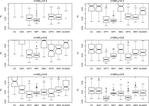5) ) for assessment. The number of simulation runs is 200. Figures 1–3 present the KL loss boxplots for each method under different simulation settings. The main conclusions are as follows.

1. The SAIC, SBIC and CC methods perform much worse than OPT1 and OPT2. In many situations, these three methods perform quite similar, indicating that SAIC and SBIC tend to select the model with more covariates and smaller sample size ($M_1$ with CC data).

2. The zero imputation methods IMP1 and IMP2 generally perform not as well as the proposed methods OPT1 and OPT2. Some exceptions happen when n and ρ are small (for example, the first panel in Figure 1), in which the usage of zeros to replace unavailable covariates has relatively small effect on the prediction.

3. The performance of GLASSO is also worse than the proposed methods, which shows the model selection method does not work quite well when the models are misspecified.

4. The proposed method OPT1 produces the lowest KL loss in most situations.

Figure 1. The KLs of all the methods in 200 replications when $\text{β}=0.4\times (1,1/2,\dots ,1/p)$.

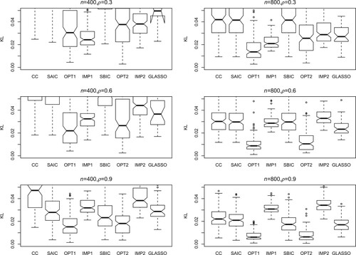
Figure 2. The KLs of all the methods in 200 replications when $\text{β}=0.1\times (1,1,\dots ,1)$.

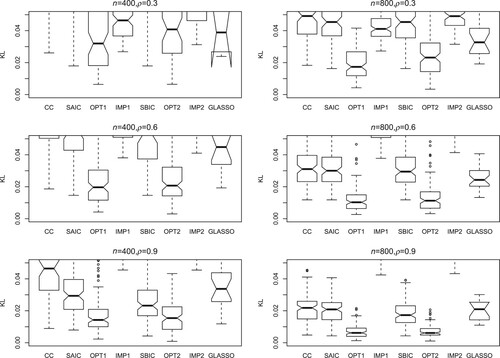
Figure 3. The KLs of all the methods in 200 replications when $\text{β}=0.2\times (1/p,\dots ,1/2,1)$.

5. A real data example

To illustrate the application of our proposed method, we consider the ADNI data which is available at http://adni.loni.usc.edu. The ADNI data contains three different phases: ADNI1, ADNIGO, and ADNI2. In this paper, we use ADNI2 in which some new model data are added. For every subject, different visits at longitudinal time points are recorded and here we focus on the baseline data. As we have mentioned in Section 1, the ADNI data mainly includes four different sources: CSF, PET, MRI and GENE. The CSF data includes 3 variables: ABETA, TAU and PTAU. Quantitative variables from the PET images are computed by Helen Wills Neuroscience Institute, UC Berkeley and Lawrence Berkeley National Laboratory containing 241 variables. The MRI is segmented and analysed in FreeSurfer by the Center for Imaging of Neurodegenerative Diseases at the University of California -- San Francisco, which produces 341 variables on volume, surface area, and thickness of regions of interest. GENE, which plays an important role in AD, contains 49,386 variables.

The overall sample size is 1170. The K = 8 response patterns and sample size for each pattern are presented in Table 2. The total missing rate is about $65\mathrm{\%}$. The MMSE provides a picture of an individual's present cognitive performance based on direct observation of completion of test items. A score of $<28$ is the general cutoff indicating the presence of cognitive impairment. As a result, we classify the MMSE score into two levels and consider the binary response Y = 1 if the MMSE score is no less than 28 and Y = 0 otherwise.

It can be seen that the data is high dimensional, which may contain variables with redundant information. Thus, we first use correlation screening to select features that are most likely to be related to the response variable. All the 3 variables in CSF are kept and 10 variables each for PET, MRI and GENE are screened. We also tried other variable number but found that this screening procedure gave us the smallest KL loss.

To compare the prediction performances of the methods considered in the simulation, we randomly select $75\mathrm{\%}$ of the subjects from each response pattern, combine them to a training data for model fitting, and use the rest of the subjects as the test data for performance evaluation. For each of the considered methods, we use the training data to fit the model, apply it to the test data, and compute the KL loss of the predictions on test data. The KL loss instead of misclassification rate is considered because the probability of AD is what we really care. We repeat this procedure independently for 100 replications.

Note that in this real data analysis, we do not only consider the prediction for $V^{\ast }=V$. For $V^{\ast }\ne \{\mathrm{C}\mathrm{S}\mathrm{F},\mathrm{P}\mathrm{E}\mathrm{T},\mathrm{M}\mathrm{R}\mathrm{I},\mathrm{G}\mathrm{E}\mathrm{N}\mathrm{E}\}$, the proposed method ignores the covariates not in $V^{\ast }$ for modelling and prediction. For example, when $V^{\ast }=\left\{\mathrm{P}\mathrm{E}\mathrm{T},\mathrm{M}\mathrm{R}\mathrm{I},\mathrm{G}\mathrm{E}\mathrm{N}\mathrm{E}\right\}$, the covariates from ‘CSF’ are ignored and only 5 candidate models are considered. More details for this kind of procedure can be found in Fang et al. (2019).

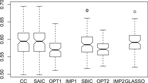
Figure 4 displays boxplots of the KL losses over 100 replications for different methods. The boxplots for IMP1 and IMP2 are not shown in the figure because their KL losses are too large. The proposed methods OPT1 and OPT2 outperform the other methods.

Figure 4. The KL loss of all the methods in 100 replications for ADNI data.

6. Concluding remarks

Fragmentary data is becoming more and more popular in many areas and it is not easy to handle. Most existing methods dealing with fragmentary data consider a continuous response while in many applications the response variable is discrete. We propose a model averaging method to deal with fragmentary data under generalized linear models. The asymptotic optimality is established and empirical results from a simulation study and a real data analysis about Alzheimer disease show the superiority of the proposed method.

There are several topics for our future study. First, the covariate dimension p and the number of candidate models K are assumed to be fixed. The asymptotic optimality with diverging p and K needs further investigation. Second, we do not focus on the comparison of ${\lambda }_n=2$ and ${\lambda }_n=\log \left(n_1\right)$. Which tuning parameter should we use in the practice? In fact, how to choose the best tuning parameter for model averaging is still a challenging problem even under linear models. Third, we assume the overall model belongs to an exponential family which is still restrictive. The extension to more general models deserves further study.

Disclosure statement

No potential conflict of interest was reported by the author(s).

Additional information

Funding

The research of Fang was supported by National Key R&D Program of China [grant numbers 2021YFA1000100, 2021YFA1000101] and National Natural Science Foundation of China [grant numbers 11831008, 12071143].

Appendix. Proof of Theorem 3.1

Proof.

Let $\tilde{\mathcal{G}}\left(w\right)=\mathcal{G}\left(w\right)-2{\varphi }^{-1}{B}_0+2{\varphi }^{-1}{\mu }_{S_1}^{\mathrm{\top }}{\theta }_0$. It is obvious that $\hat{w}={\mathrm{a}\mathrm{r}\mathrm{g}\mathrm{m}\mathrm{i}\mathrm{n}}_{w\in {\mathcal{H}}_n}\tilde{\mathcal{G}}\left(w\right)$. From the proof of Theorem 1 in Wan et al. (2010), Theorem 3.1 is valid if the following two conclusions hold: (A1) $\left(\mathrm{i}\right)\underset{w\in {\mathcal{H}}_n}{sup}\frac{|\mathrm{K}\mathrm{L}\left(w\right)-{\mathrm{K}\mathrm{L}}^{\ast }\left(w\right)|}{{\mathrm{K}\mathrm{L}}^{\ast }\left(w\right)}{\to }_{p}0,$(A1) and (A2) $\left(\mathrm{i}\mathrm{i}\right)\underset{w\in {\mathcal{H}}_n}{sup}\frac{|\tilde{\mathcal{G}}\left(w\right)-{\mathrm{K}\mathrm{L}}^{\ast }\left(w\right)|}{{\mathrm{K}\mathrm{L}}^{\ast }\left(w\right)}{\to }_{p}0.$(A2) By (6(6) ${\widehat{\text{β}}}_{\left(k\right)}-{\text{β}}_{\left(k\right)}^{\ast }=O_p\left(n_k^{-1/2}\right)=O_p\left(n_1^{-1/2}\right).$(6) ), we know that uniformly for $w\in {\mathcal{H}}_n$, (A3) $\begin{array}{r}\widehat{\text{β}}\left(w\right)-{\text{β}}^{\ast }\left(w\right)=\sum _{k=1}^K{w}_k{\mathrm{\Pi }}_k^{\mathrm{\top }}({\widehat{\text{β}}}_{\left(k\right)}-{\text{β}}_{\left(k\right)}^{\ast })=O_p\left(n_1^{-1/2}\right).\end{array}$(A3) It follows from (A3(A3) $\begin{array}{r}\widehat{\text{β}}\left(w\right)-{\text{β}}^{\ast }\left(w\right)=\sum _{k=1}^K{w}_k{\mathrm{\Pi }}_k^{\mathrm{\top }}({\widehat{\text{β}}}_{\left(k\right)}-{\text{β}}_{\left(k\right)}^{\ast })=O_p\left(n_1^{-1/2}\right).\end{array}$(A3) ), Condition (C1), and Taylor expansion that uniformly for $w\in {\mathcal{H}}_n$, $\begin{array}{rl}& |B\left\{\widehat{\text{β}}\right(w\left)\right\}-B\left\{{\text{β}}^{\ast }\right(w\left)\right\}|\\ & \le \Vert \frac{\mathrm{\partial }B\left(\text{β}\right)}{\mathrm{\partial }{\text{β}}^{\mathrm{\top }}}{|}_{\text{β}=\widetilde{\text{β}}\left(w\right)}\Vert \parallel \widehat{\text{β}}\left(w\right)-{\text{β}}^{\ast }\left(w\right)\parallel =O_p\left(n_1^{1/2}\right),\\ & {\mu }_{S_1}^{\mathrm{\top }}\left[\theta \right\{\widehat{\text{β}}\left(w\right)\}-\theta \{{\text{β}}^{\ast }\left(w\right)\left\}\right]\\ & \le \parallel {\mu }_{S_1}^{\mathrm{\top }}{\mathrm{X}}_1\parallel \parallel \widehat{\text{β}}\left(w\right)-{\text{β}}^{\ast }\left(w\right)\parallel =O_p\left(n_1^{1/2}\right),\end{array}$ and $\begin{array}{rl}& {ϵ}_{S_1}^{\mathrm{\top }}\left[\theta \right\{\widehat{\text{β}}\left(w\right)\}-\theta \{{\text{β}}^{\ast }\left(w\right)\left\}\right]\\ & \le \parallel {ϵ}_{S_1}^{\mathrm{\top }}{\mathrm{X}}_1\parallel \parallel \widehat{\text{β}}\left(w\right)-{\text{β}}^{\ast }\left(w\right)\parallel =O_p\left(1\right),\end{array}$ where $\widetilde{\text{β}}\left(w\right)$ is a vector between $\widehat{\text{β}}\left(w\right)$ and ${\text{β}}^{\ast }\left(w\right)$. In addition, using the central limit theorem and Condition (C.2), we know that uniformly for $w\in {\mathcal{H}}_n$, ${ϵ}_{S_1}^{\mathrm{\top }}\theta \left\{{\text{β}}^{\ast }\right(w\left)\right\}=\sum _{k=1}^K{w}_k{ϵ}_{S_1}^{\mathrm{\top }}\theta \left({\mathrm{\Pi }}_k^{\mathrm{\top }}{\text{β}}_{\left(k\right)}^{\ast }\right)=O_p\left(n_1^{1/2}\right).$

Then we have (A4) $\begin{array}{rl}& \underset{w\in {\mathcal{H}}_n}{sup}|\mathrm{K}\mathrm{L}\left(w\right)-{\mathrm{K}\mathrm{L}}^{\ast }\left(w\right)|\\ & \le 2{\varphi }^{-1}\underset{w\in {\mathcal{H}}_n}{sup}|B\left\{\widehat{\text{β}}\right(w\left)\right\}-B\left\{{\text{β}}^{\ast }\right(w\left)\right\}|\\ & +2{\varphi }^{-1}\underset{w\in {\mathcal{H}}_n}{sup}|{\mu }_{S_1}^{\mathrm{\top }}\left[\theta \right\{\widehat{\text{β}}\left(w\right)\}-\theta \{{\text{β}}^{\ast }\left(w\right)\left\}\right]|\\ & =O_p\left(n_1^{1/2}\right)\end{array}$(A4) and (A5) $\begin{array}{rl}& \underset{w\in {\mathcal{H}}_n}{sup}|\tilde{\mathcal{G}}\left(w\right)-{\mathrm{K}\mathrm{L}}^{\ast }\left(w\right)|\\ & \le 2{\varphi }^{-1}\underset{w\in {\mathcal{H}}_n}{sup}|B\left\{\widehat{\text{β}}\right(w\left)\right\}-B\left\{{\text{β}}^{\ast }\right(w\left)\right\}|\\ & +2{\varphi }^{-1}\underset{w\in {\mathcal{H}}_n}{sup}|y_{S_1}^{\mathrm{\top }}\theta \left\{\widehat{\text{β}}\right(w\left)\right\}-{\mu }_{S_1}^{\mathrm{\top }}\theta \left\{{\text{β}}^{\ast }\right(w\left)\right\}|\\ & +{\lambda }_n\sum _{k=1}^K{w}_k{p}_k\\ & \le 2{\varphi }^{-1}\underset{w\in {\mathcal{H}}_n}{sup}|B\left\{\widehat{\text{β}}\right(w\left)\right\}-B\left\{{\text{β}}^{\ast }\right(w\left)\right\}|\\ & +2{\varphi }^{-1}\underset{w\in {\mathcal{H}}_n}{sup}|{\mu }_{S_1}^{\mathrm{\top }}\left[\theta \right\{\widehat{\text{β}}\left(w\right)\}-\theta \{{\text{β}}^{\ast }\left(w\right)\left\}\right]|\\ & +2{\varphi }^{-1}\underset{w\in {\mathcal{H}}_n}{sup}|{ϵ}_{S_1}^{\mathrm{\top }}\theta \left\{{\text{β}}^{\ast }\right(w\left)\right\}|\\ & +2{\varphi }^{-1}\underset{w\in {\mathcal{H}}_n}{sup}|{ϵ}_{S_1}^{\mathrm{\top }}\left[\theta \right\{\widehat{\text{β}}\left(w\right)\}-\theta \{{\text{β}}^{\ast }\left(w\right)\left\}\right]|\\ & +{\lambda }_n\sum _{k=1}^K{w}_k{p}_k\\ & =O_p\left(n_1^{1/2}\right)+{\lambda }_n\sum _{k=1}^K{w}_k{p}_k.\end{array}$(A5) Now, from (A4(A4) $\begin{array}{rl}& \underset{w\in {\mathcal{H}}_n}{sup}|\mathrm{K}\mathrm{L}\left(w\right)-{\mathrm{K}\mathrm{L}}^{\ast }\left(w\right)|\\ & \le 2{\varphi }^{-1}\underset{w\in {\mathcal{H}}_n}{sup}|B\left\{\widehat{\text{β}}\right(w\left)\right\}-B\left\{{\text{β}}^{\ast }\right(w\left)\right\}|\\ & +2{\varphi }^{-1}\underset{w\in {\mathcal{H}}_n}{sup}|{\mu }_{S_1}^{\mathrm{\top }}\left[\theta \right\{\widehat{\text{β}}\left(w\right)\}-\theta \{{\text{β}}^{\ast }\left(w\right)\left\}\right]|\\ & =O_p\left(n_1^{1/2}\right)\end{array}$(A4) ) to (A5(A5) $\begin{array}{rl}& \underset{w\in {\mathcal{H}}_n}{sup}|\tilde{\mathcal{G}}\left(w\right)-{\mathrm{K}\mathrm{L}}^{\ast }\left(w\right)|\\ & \le 2{\varphi }^{-1}\underset{w\in {\mathcal{H}}_n}{sup}|B\left\{\widehat{\text{β}}\right(w\left)\right\}-B\left\{{\text{β}}^{\ast }\right(w\left)\right\}|\\ & +2{\varphi }^{-1}\underset{w\in {\mathcal{H}}_n}{sup}|y_{S_1}^{\mathrm{\top }}\theta \left\{\widehat{\text{β}}\right(w\left)\right\}-{\mu }_{S_1}^{\mathrm{\top }}\theta \left\{{\text{β}}^{\ast }\right(w\left)\right\}|\\ & +{\lambda }_n\sum _{k=1}^K{w}_k{p}_k\\ & \le 2{\varphi }^{-1}\underset{w\in {\mathcal{H}}_n}{sup}|B\left\{\widehat{\text{β}}\right(w\left)\right\}-B\left\{{\text{β}}^{\ast }\right(w\left)\right\}|\\ & +2{\varphi }^{-1}\underset{w\in {\mathcal{H}}_n}{sup}|{\mu }_{S_1}^{\mathrm{\top }}\left[\theta \right\{\widehat{\text{β}}\left(w\right)\}-\theta \{{\text{β}}^{\ast }\left(w\right)\left\}\right]|\\ & +2{\varphi }^{-1}\underset{w\in {\mathcal{H}}_n}{sup}|{ϵ}_{S_1}^{\mathrm{\top }}\theta \left\{{\text{β}}^{\ast }\right(w\left)\right\}|\\ & +2{\varphi }^{-1}\underset{w\in {\mathcal{H}}_n}{sup}|{ϵ}_{S_1}^{\mathrm{\top }}\left[\theta \right\{\widehat{\text{β}}\left(w\right)\}-\theta \{{\text{β}}^{\ast }\left(w\right)\left\}\right]|\\ & +{\lambda }_n\sum _{k=1}^K{w}_k{p}_k\\ & =O_p\left(n_1^{1/2}\right)+{\lambda }_n\sum _{k=1}^K{w}_k{p}_k.\end{array}$(A5) ), $n_1{\xi }_n^{-2}=o\left(1\right)$, and $n_1^{-1/2}{\lambda }_n=O\left(1\right)$, we can obtain (A1(A1) $\left(\mathrm{i}\right)\underset{w\in {\mathcal{H}}_n}{sup}\frac{|\mathrm{K}\mathrm{L}\left(w\right)-{\mathrm{K}\mathrm{L}}^{\ast }\left(w\right)|}{{\mathrm{K}\mathrm{L}}^{\ast }\left(w\right)}{\to }_{p}0,$(A1) ) and (A2(A2) $\left(\mathrm{i}\mathrm{i}\right)\underset{w\in {\mathcal{H}}_n}{sup}\frac{|\tilde{\mathcal{G}}\left(w\right)-{\mathrm{K}\mathrm{L}}^{\ast }\left(w\right)|}{{\mathrm{K}\mathrm{L}}^{\ast }\left(w\right)}{\to }_{p}0.$(A2) ). This completes the proof.

References

- Akaike, H. (1970). Statistical predictor identification. Annals of the Institute of Statistical Mathematics, 22(1), 203–217. https://doi.org/10.1007/BF02506337
- Ando, T., & Li, K.-C. (2014). A model averaging approach for high dimensional regression. Journal of American Statistical Association, 109(505), 254–265. https://doi.org/10.1080/01621459.2013.838168
- Ando, T., & Li, K.-C. (2017). A weight-relaxed model averaging approach for high-dimensional generalized linear models. The Annals of Statistics, 45(6), 2654–2679. https://doi.org/10.1214/17-AOS1538
- Buckland, S. T., Burnham, K. P., & Augustin, N. H. (1997). Model selection: An integral part of inference. Biometrics, 53(2), 603–618. https://doi.org/10.2307/2533961
- Chen, J., Li, D., Linton, O., & Lu, Z. (2018). Semiparametric ultra-high dimensional model averaging of nonlinear dynamic time series. Journal of the American Statistical Association, 113(522), 919–932. https://doi.org/10.1080/01621459.2017.1302339
- Dardanoni, V., Luca, G. D., Modica, S., & Peracchi, F. (2015). Model averaging estimation of generalized linear models with imputed covariates. Journal of Econometrics, 184(2), 452–463. https://doi.org/10.1016/j.jeconom.2014.06.002
- Dardanoni, V., Modica, S., & Peracchi, F. (2011). Regression with imputed covariates: A generalized missing indicator approach. Journal of Econometrics, 162(2), 362–368. https://doi.org/10.1016/j.jeconom.2011.02.005
- Ding, X., Xie, J., & Yan, X. (2021). Model averaging for multiple quantile regression with covariates missing at random. Journal of Statistical Computation and Simulation, 91(11), 2249–2275. https://doi.org/10.1080/00949655.2021.1890733
- Fan, J., & Li, R. (2001). Variable selection via nonconcave penalized likelihood and its oracle properties. Journal of American Statistical Association, 96(456), 1348–1360. https://doi.org/10.1198/016214501753382273
- Fan, J., & Lv, J. (2008). Sure independence screening for ultrahigh dimensional feature space (with discussions). Journal of the Royal Statistical Society: Series B (Statistical Methodology), 70(5), 849–911. https://doi.org/10.1111/rssb.2008.70.issue-5
- Fang, F., Li, J., & Xia, X. (2022). Semiparametric model averaging prediction for dichotomous response. Journal of Econometrics, 229(2), 219–245. https://doi.org/10.1016/j.jeconom.2020.09.008
- Fang, F., Wei, L., Tong, J., & Shao, J. (2019). Model averaging for prediction with fragmentary data. Journal of Business & Economic Statistics, 37(3), 517–527. https://doi.org/10.1080/07350015.2017.1383263
- Hansen, B. E. (2007). Least squares model averaging. Econometrica, 75(4), 1175–1189. https://doi.org/10.1111/ecta.2007.75.issue-4
- Hansen, B. E., & Racine, J. S. (2012). Jackknife model averaging. Journal of Econometrics, 167(1), 38–46. https://doi.org/10.1016/j.jeconom.2011.06.019
- Hjort, N. L., & Claeskens, G. (2003). Frequentist model average estimators. Journal of American Statistical Association, 98(464), 879–899. https://doi.org/10.1198/016214503000000828
- Hoeting, J., Madigan, D., Raftery, A., & Volinsky, C. (1999). Bayesian model averaging: A tutorial. Statistical Science, 14(4), 382–401. https://doi.org/10.1214/ss/1009212519
- Kim, J. K., & Shao, J. (2013). Statistical methods for handling incomplete data. Chapman & Hall/CRC.
- Leung, G., & Barron, A. R. (2006). Information theory and mixing least-squares regressions. IEEE Transactions on Information Theory, 52(8), 3396–3410. https://doi.org/10.1109/TIT.2006.878172
- Li, C., Li, Q., Racine, J. S., & Zhang, D. (2018). Optimal model averaging of varying coefficient models. Statistica Sinica, 28(2), 2795–2809. https://doi.org/10.5705/ss.202017.0034
- Li, D., Linton, O., & Lu, Z. (2015). A flexible semiparametric forecasting model for time series. Journal of Econometrics, 187(1), 345–357. https://doi.org/10.1016/j.jeconom.2015.02.025
- Liao, J., Zong, X., Zhang, X., & Zou, G. (2019). Model averaging based on leave-subject-out cross-validation for vector autoregressions. Journal of Econometrics, 209(1), 35–60. https://doi.org/10.1016/j.jeconom.2018.10.007
- Lin, H., Liu, W., & Lan, W. (2021). Regression analysis with individual-specific patterns of missing covariates. Journal of Business & Economic Statistics, 39(1), 179–188. https://doi.org/10.1080/07350015.2019.1635486
- Little, R. J. A., & Rubin, D. B. (2002). Statistical analysis with missing data. 2nd ed. Wiley.
- Liu, Q., & Okui, R. (2013). Heteroskedasticity-robust Cp model averaging. The Econometrics Journal, 16(3),463–472. https://doi.org/10.1111/ectj.12009
- Liu, Q., & Zheng, M. (2020). Model averaging for generalized linear model with covariates that are missing completely at random. The Journal of Quantitative Economics, 11(4), 25–40. https://doi.org/10.16699/b.cnki.jqe.2020.04.003
- Longford, N. T. (2005). Editorial: Model selection and efficiency is ‘Which model…?’ the right question? Journal of the Royal Statistical Society: Series A (Statistics in Society), 168(3), 469–472. https://doi.org/10.1111/rssa.2005.168.issue-3
- Lu, X., & Su, L. (2015). Jackknife model averaging for quantile regressions. Journal of Econometrics, 188(1), 40–58. https://doi.org/10.1016/j.jeconom.2014.11.005
- Mallows, C. (1973). Some comments on Cp. Technometrics, 15(4), 661–675. https://doi.org/10.2307/1267380
- Meier, L., Geer, S. V. D., & Peter, B. (2008). The group lasso for logistic regression. Journal of the Royal Statistical Society: Series B (Statistical Methodology), 70(1), 53–71. https://doi.org/10.1111/j.1467-9868.2007.00627.x
- Schomaker, M., Wan, A. T. K., & Heumann, C. (2010). Frequentist model averaging with missing observations. Computational Statistics and Data Analysis, 54(12), 3336–3347. https://doi.org/10.1016/j.csda.2009.07.023
- Schwarz, G. (1978). Estimating the dimension of a model. The Annals of Statistics, 6(2), 461–464. https://doi.org/10.1214/aos/1176344136
- Tibshirani, R. (1996). Regression shrinkage and selection via the lasso. Journal of the Royal Statistical Society: Series B (Methodological), 58(1), 267–288. https://doi.org/10.1111/j.2517-6161.1996.tb02080.x
- Wan, A. T. K., Zhang, X., & Zou, G. (2010). Least squares model averaging by Mallows criterion. Journal of Econometrics, 156(2), 277–283. https://doi.org/10.1016/j.jeconom.2009.10.030
- White, H. (1982). Maximum likelihood estimation of misspecified models. Econometrica, 50(1), 1–25. https://doi.org/10.2307/1912526
- Xue, F., & Qu, A. (2021). Integrating multi-source block-wise missing data in model selection. Journal of American Statistical Association, 116(536), 1914–1927. https://doi.org/10.1080/01621459.2020.1751176
- Yang, Y. (2001). Adaptive regression by mixing. Journal of American Statistical Association, 96(454), 574–588. https://doi.org/10.1198/016214501753168262
- Yang, Y. (2003). Regression with multiple candidate models: Selecting or mixing? Statistica Sinica, 13, 783–809.
- Zhang, X. (2013). Model averaging with covariates that are missing completely at random. Economics Letters, 121(3), 360–363. https://doi.org/10.1016/j.econlet.2013.09.008
- Zhang, X., Yu, D., Zou, G., & Liang, H. (2016). Optimal model averaging estimation for generalized linear models and generalized linear mixed-effects models. Journal of the American Statistical Association, 111(516), 1775–1790. https://doi.org/10.1080/01621459.2015.1115762
- Zhang, X., Zou, G., & Liang, H. (2014). Model averaging and weight choice in linear mixed effects models. Biometrika, 101(1), 205–218. https://doi.org/10.1093/biomet/ast052
- Zhang, X., Zou, G., Liang, H., & Carroll, R. J. (2020). Parsimonious model averaging with a diverging number of parameters. Journal of the American Statistical Association, 115(530), 972–984. https://doi.org/10.1080/01621459.2019.1604363
- Zhang, Y., Tang, N., & Qu, A. (2020). Imputed factor regression for high-dimensional block-wise missing data. Statistica Sinica, 30(2), 631–651. https://doi.org/10.5705/ss.202018.0008
- Zheng, H., Tsui, K-W, Kang, X., & Deng, X. (2017). Cholesky-based model averaging for covariance matrix estimation. Statistical Theory and Related Fields, 1(1), 48–58. https://doi.org/10.1080/24754269.2017.1336831
- Zhu, R., Wan, A. T. K., Zhang, X., & Zou, G. (2019). A Mallow-type model averaging estimator for the varying-coefficient partially linear model. Journal of the American Statistical Association, 114(526), 882–892. https://doi.org/10.1080/01621459.2018.1456936