Variable selection in finite mixture of median regression models using skew-normal distribution

Abstract

A regression model with skew-normal errors provides a useful extension for traditional normal regression models when the data involve asymmetric outcomes. Moreover, data that arise from a heterogeneous population can be efficiently analysed by a finite mixture of regression models. These observations motivate us to propose a novel finite mixture of median regression model based on a mixture of the skew-normal distributions to explore asymmetrical data from several subpopulations. With the appropriate choice of the tuning parameters, we establish the theoretical properties of the proposed procedure, including consistency for variable selection method and the oracle property in estimation. A productive nonparametric clustering method is applied to select the number of components, and an efficient EM algorithm for numerical computations is developed. Simulation studies and a real data set are used to illustrate the performance of the proposed methodologies.

Keywords:

• Variable selection
• mixture of median regression
• skew-normal distribution
• heterogeneous population
• EM algorithm

1. Introduction

When the data involve asymmetrical outcomes, inference under the linear regression model with the skewed random errors can be viewed as an alternative procedure to the classical regression models with symmetric errors, since the use of a skewed distribution for the errors could reduce the influence of outliers and thus make statistical analysis more robust. Specifically, suppose that a response variable Y given a set of predictors $\mathit{x}$ takes the form of (1) $y={\mathit{x}}^{\mathrm{\top }}\text{β}+ϵ,$(1) where $\text{β}$ represents a vector of the unknown regression coefficients and the conditional density of the error term ϵ given $\mathit{x}$ follows an unknown distribution with the probability density function (pdf) $g(ϵ\mid \mathit{x})$. It is known that if $g(ϵ\mid \mathit{x})$ is symmetrical about 0, the estimation of β in (1(1) $y={\mathit{x}}^{\mathrm{\top }}\text{β}+ϵ,$(1) ) will be the same as the coefficients obtained by conventional mean linear regression. However, if $g(ϵ\mid \mathit{x})$ is skewed, the median regression provides a more reliable statistical analysis with adaptive robustness to outliers, since the median of a distribution is less susceptible to outliers, especially when the data involve asymmetrical outcomes. We here refer the interested readers to Kottas and Gelfand (2001), Zhou and Liu (2016) and Hu et al. (2019) for relevant research on the median regression of population distributions.

It is noteworthy to mention that the median regression has been widely used for studying the relationship between the response variable Y and a set of predictors $\mathit{x}$ in symmetrical distribution, whereas such a median regression may not be suitable for analysing the data exhibiting asymmetrical behaviour or the data that arise from a heterogeneous population. To tackle this difficulty, mixture of regression models (known as switching regression models in econometrics), initially introduced by Goldfeld and Quandt (1973), may be employed as a flexible tool for studying the skewed data from two or more subpopulations. Since then, finite mixture of regression (FMR) models has been widely used in a variety of fields including but not limited to biology, medicine, economics, environmental science, sampling survey and engineering technology. The book by McLachlan and Peel (2004) contains a comprehensive review of FMR models. An FMR model is obtained when a response variable with a finite mixture distribution depends on a set of covariates, and FMR models have been discussed extensively when the normality is assumed for the regression error in each component.

However, it has been shown that the commonly used normal mixture model tends to be an over fitting model, since additional components are usually needed to capture the skewness of the data. To overcome the potential inappropriateness of normal mixtures in some context, we may consider the use of the skew-normal distributions (Azzalini, 1985) as component densities of the errors; see, for example, Wu et al. (2013), Wu (2014), Tang and Tang (2015), and H. Li et al. (2016, 2017), to name just a few. These observations motivate us to develop a novel finite mixture of the median regression (FMMeR) model based on a mixture of the skew-normal distributions to explore asymmetrical data that arise from several subpopulations. There exist two barriers for the development of the FMMeR model. The first barrier is to deal with computational aspects of parameter estimation when fitting the FMMeR model with the skew-normal distribution for the errors. We tackle this barrier by utilizing the stochastic representation and hierarchical representation (see, for example, Liu & Lin, 2014) of skew-normal mixtures. A second technical barrier is to determine the number of components of the FMMeR model under consideration. Popularly, the log-likelihood maximum and two information-based criteria, AIC (Akaike, 1973) and BIC (Schwarz, 1978), can be used to select the number of components. Although some success has been shown using the model choice criteria, choosing the right number of components for a mixture model is known to be difficult. Thus, we consider a procedure of clustering to determine the number of components, which has been shown to be very effective via real-data example, and it is introduced in Subsection 5.3.

To enhance predictability and to give a concise model, it is reasonable to include only the significant covariates in the model. As a result, variable selection has also become increasingly important for FMR models and a rich literature has been generated in recent several decades. All-subset selection methods, such as the AIC and BIC, and their modifications, have been widely investigated in the context of FMR models; for instance, P. Wang et al. (1996) researched model selection in a finite mixture of Poisson regression models via AIC and BIC. However, all-subset selection methods for FMR models are computationally intensive. To improve computational efficiency, the least absolute shrinkage and selection operator (LASSO) of Tibshirani (1996) and the smoothly clipped absolute deviation (SCAD) method of Fan and Li (2001) are proposed as new methods for variable selection. The penalized likelihood for FMR models, the extension of penalized least square methods, were proposed by Khalili and Chen (2007). Recently, Wu et al. (2020) proposed an estimation and variable selection method for mixture of joint mean and variance models; Yin, Wu, and Dai (2020) proposed variable selection procedures in FMR models using the skew-normal distribution.

The remainder of this paper is organized as follows. In Section 2, we briefly introduce the skew-normal distribution and its median expression. In Section 3, we develop a variable selection method for FMMeR model via the penalized likelihood-based procedure for analysing asymmetrical data from several subpopulations. Section 4 studies asymptotic properties of the resulting estimators. In Section 5, a numerical algorithm, a productive nonparametric clustering method for determining the number of components and a data-adaptive method for choosing tuning parameters are discussed. In Section 6, we carry out simulation studies to investigate the finite sample performance of the proposed methodology. A real-data example is provided in Section 7 for illustrative purposes. Some concluding remarks are given in Section 8. Brief proofs of theorems and some technical derivations are given in Appendices 1 and 2.

2. The skew-normal mixture of median regression models

2.1. Skew-normal distribution

A random variable Y is said to follow a univariate skew-normal distribution with location parameter μ, scale parameter $\sigma \in (0,\mathrm{\infty })$ and skewness parameter $\lambda \in \mathbb{R}$, denoted by $Y\sim SN(\mu ,{\sigma }^2,\lambda )$, if its pdf is given by (2) $f(y\mid \mu ,{\sigma }^2,\lambda )=\frac{2}{\sigma }\varphi \left(\frac{y-\mu }{\sigma }\right)\mathrm{\Phi }\left(\lambda \left(\frac{y-\mu }{\sigma }\right)\right),$(2) where $\varphi (\cdot )$ and $\mathrm{\Phi }(\cdot )$ denote the pdf and cumulative distribution function (cdf) of the standard normal distribution, respectively. It is worth noting that if $\lambda =0$, the density of Y reduces to a normal density $N(\mu ,{\sigma }^2)$ and that the distribution is positively skewed if $\lambda >0$ and is negatively skewed if $\lambda <0$.

We represent the skew-normal distribution in an incomplete data framework. Specifically, the stochastic representation for random variable $Y\sim SN(\mu ,{\sigma }^2,\lambda )$ is given by (3) $Y_i=\mu +\sigma \left(\delta \right(\lambda )R_i+\sqrt{1-{\delta }^2\left(\lambda \right)}{V}_i),$(3)

where $i=1,\dots ,n$ with a sample size of n, $\delta \left(\lambda \right)=\lambda /\sqrt{1+{\lambda }^2}$. Here, $R_i\sim TN(0,1)I\{r_i>0\}$ and $V_i\sim N(0,1)$, where $R_i$ and $V_i$ are independent. $R\sim TN(\mu ,{\sigma }^2)I\{a_1<r<a_2\}$ is a truncated normal distribution with the density $\begin{array}{r}{f}_R(r\mid \mu ,{\sigma }^2)={\{\mathrm{\Phi }\left(\frac{a_2-\mu }{\sigma }\right)-\mathrm{\Phi }\left(\frac{a_1-\mu }{\sigma }\right)\}}^{-1}\times \frac{1}{\sqrt{2\text{π}}\sigma }\exp \{-\frac{1}{2{\sigma }^2}(r-\mu {)}^2\},\end{array}$where $a_1<r<a_2$ and $I\{\cdot \}$ represents an indicator function. For notational simplicity, let $\mathit{Y}=(Y_1,\dots ,Y_n{)}^{\mathrm{\top }}$ and $\mathit{R}=(R_1,\dots ,R_n{)}^{\mathrm{\top }}$. Furthermore, the skew-normal distribution can be decomposed into a normal distribution and a truncated normal distribution by a hierarchical representation given by (4) $\begin{array}{rl}{Y}_i\mid R_i=r_i& \sim N(\mu +\sigma r_i\delta \left(\lambda \right),{\sigma }^2(1-{\delta }^2(\lambda \left)\right)),\\ R_i& \sim TN(0,1)I\{r_i>0\}.\end{array}$(4) Azzalini and Capitanio (2013) adopted the moment-generating function to calculate the mean and variance for the skew-normal distribution in (2(2) $f(y\mid \mu ,{\sigma }^2,\lambda )=\frac{2}{\sigma }\varphi \left(\frac{y-\mu }{\sigma }\right)\mathrm{\Phi }\left(\lambda \left(\frac{y-\mu }{\sigma }\right)\right),$(2) ) and they are given by (5) $E\left(Y\right)=\mu +{\mu }_0\left(\lambda \right)\sigma ,\mathrm{V}\mathrm{a}\mathrm{r}\left(Y\right)={\sigma }_0^2\left(\lambda \right){\sigma }^2,$(5) respectively, where ${\mu }_0\left(\lambda \right)\widehat{=}\sqrt{2/\pi }\delta \left(\lambda \right)$ and ${\sigma }_0^2\left(\lambda \right)\widehat{=}1-{\mu }_0^2\left(\lambda \right)$. Of particular note is that Lin et al. (2007) introduced a simple way of obtaining higher moments of the skew-normal distribution without the use of its moment-generating function. Letting $m_0\left(\lambda \right)$ be the mode of the distribution $SN(0,1,\lambda )$, a quite accurate approximation of $m_0\left(\lambda \right)$ evaluated by the numerical maximization method is given by $\begin{array}{r}{m}_0\left(\lambda \right)\approx {\mu }_0\left(\lambda \right)-\frac{t_0\left(\lambda \right){\sigma }_0\left(\lambda \right)}{2}-\frac{\mathrm{s}\mathrm{i}\mathrm{g}\mathrm{n}\left(\lambda \right)}{2}\exp \{-\frac{2\pi }{|\lambda |}\},\end{array}$where $\mathrm{s}\mathrm{i}\mathrm{g}\mathrm{n}\left(\lambda \right)$ indicates the sign function for λ and $t_0\left(\lambda \right)\widehat{=}\frac{4-\text{π}}{2}\frac{{\mu }_0^3\left(\lambda \right)}{{\sigma }_0^3\left(\lambda \right)}.$It deserves mentioning that the logarithm of the density for the skew-normal distribution is a concave function and that this property is not altered by a change of location and scale parameters. Thus, $m_0\left(\lambda \right)$ is unique and the mode of the skew-normal distribution in (2(2) $f(y\mid \mu ,{\sigma }^2,\lambda )=\frac{2}{\sigma }\varphi \left(\frac{y-\mu }{\sigma }\right)\mathrm{\Phi }\left(\lambda \left(\frac{y-\mu }{\sigma }\right)\right),$(2) ) can be reexpressed as $\mathrm{M}\mathrm{o}\mathrm{d}\mathrm{e}\left(Y\right)=\mu +m_0\left(\lambda \right)\sigma$. Mean(Y), Mode(Y) and Median(Y) have the quantitative relationship when the observations follow a skew-normal distribution: $\mathrm{M}\mathrm{e}\mathrm{d}\mathrm{i}\mathrm{a}\mathrm{n}\left(Y\right)\approx \left[\mathrm{M}\mathrm{o}\mathrm{d}\mathrm{e}\right(Y)+2\mathrm{M}\mathrm{e}\mathrm{a}\mathrm{n}(Y\left)\right]/3$, that is, (6) $\mathrm{M}\mathrm{e}\mathrm{a}\mathrm{d}\mathrm{i}\mathrm{a}\mathrm{n}\left(Y\right)\approx \mu +\frac{\left[m_0\right(\lambda )+2{\mu }_0(\lambda \left)\right]\sigma }{3},$(6) which could facilitate the development of the median regression with the skew-normal mixtures discussed below.

2.2. Median regression for skew-normal mixtures

In this paper, we assume that the response variable $Y_i$ follows a skew-normal distribution with location parameter ${\mu }_i$, scale parameter σ and skewness parameter λ, denoted by $Y_i\sim SN({\mu }_i,{\sigma }^2,\lambda )$ for $i=1,\dots ,n$. A linear mode regression model with skew-normal errors can be expressed as (7) $y_i={\mathit{x}}_i^{\mathrm{\top }}\text{β}+{ϵ}_i,$(7) where $\mathrm{M}\mathrm{e}\mathrm{d}\mathrm{i}\mathrm{a}\mathrm{n}(Y_i\mid \mathit{X})={\mathit{x}}_i^{\mathrm{\top }}\text{β}={\mu }_i+\left[m_0\right(\lambda )+2{\mu }_0(\lambda \left)\right]\sigma /3$ defined by (6(6) $\mathrm{M}\mathrm{e}\mathrm{a}\mathrm{d}\mathrm{i}\mathrm{a}\mathrm{n}\left(Y\right)\approx \mu +\frac{\left[m_0\right(\lambda )+2{\mu }_0(\lambda \left)\right]\sigma }{3},$(6) ). Here $\mathit{X}=({\mathit{x}}_1,\dots ,{\mathit{x}}_n)$ is a $p\times n$ design matrix, such that each of its element ${\mathit{x}}_i=(x_{i1},\dots ,x_{ip}{)}^{\mathrm{\top }}$ is the p-dimensional vector of predictors, and $\text{β}=({\text{β}}_1,\dots ,{\text{β}}_p{)}^{\mathrm{\top }}$ is a p-dimensional vector of the unknown regression coefficients, and $\mathit{ϵ}=({ϵ}_1,\dots ,{ϵ}_n{)}^{\mathrm{\top }}$ stands for the n-dimensional vector of random errors such that ${ϵ}_i\stackrel{iid}{\sim }SN(-[m_0\left(\lambda \right)+2{\mu }_0\left(\lambda \right)]\sigma /3,{\sigma }^2,\lambda )$.

We consider the case where the data from heterogeneous populations. A finite mixture median regression (FMMeR) model with m-components of the skew-normal distributions is defined as (8) $\{\begin{array}{rl}f(y_i\mid \mathbf{\Psi })& ={\displaystyle \sum _{j=1}^m{\nu }_{j}SN(y_i\mid {\mu }_{ij},{\sigma }_j^2,{\lambda }_j),i=1,2,\dots ,n,j=1,2,\dots ,m,}\\ \mathrm{M}\mathrm{e}\mathrm{d}\mathrm{i}\mathrm{a}\mathrm{n}\left(y_{ij}\right)& ={\mathit{x}}_i^{\mathrm{\top }}{\text{β}}_j,\end{array}$(8) where $SN(y_i\mid {\mu }_{ij},{\sigma }_j^2,{\lambda }_j)=\frac{2}{{\sigma }_j}\varphi \left(\frac{y_i-{\mu }_j}{{\sigma }_j}\right)\mathrm{\Phi }\left({\lambda }_j\frac{y_i-{\mu }_j}{{\sigma }_j}\right),$$\mathit{\nu }=({\nu }_1,\dots ,{\nu }_m{)}^{\mathrm{\top }}$ are the mixing proportions which are constrained to be non-negative and sum to unity, ${\text{β}}_{\mathit{j}}=({\text{β}}_{j1},\dots ,{\text{β}}_{jp}{)}^{\mathrm{\top }}$ and $\mathbf{\Psi }=({\nu }_1,\dots ,{\nu }_{m-1},{\text{β}}_1^{\mathrm{\top }},\dots ,{\text{β}}_m^{\mathrm{\top }},{\sigma }_1,\dots ,{\sigma }_m,{\lambda }_1,\dots ,{\lambda }_m{)}^{\mathrm{\top }}$. It is obvious that (9) ${\mu }_{ij}={\mathit{x}}_i^{\mathrm{\top }}{\text{β}}_j-\frac{{\sigma }_j}{3}\left[m_0\right({\lambda }_j)+2\sqrt{\frac{2}{\text{π}}}\delta ({\lambda }_j\left)\right],$(9) which shows that the location in the FMMeR model is altered by a change of scale and skewness parameters.

2.3. Identifiability

An important part associated with statistical inference for FMR models is their identifiability. It is well known that mixture models are not absolutely identifiable in general. However, in some mixture model settings, it is possible to establish a weaker sense of identifiability. Titterington et al. (1985) have given relevant conclusions that the FMR models of continuous distribution are identifiable in most cases. Otiniano et al. (2015) introduced the identifiability of finite mixture of skew-normal distribution and gave detailed explanation. The cumulative distribution function of Y is denoted by $F_Y$. It is possible to define the skew-normal family as the set $\mathcal{F}=\{F:F_Y(y\mid \mu ,{\sigma }^2,\lambda )={\int }_{-\mathrm{\infty }}^{y}f(t\mid \mu ,{\sigma }^2,\lambda \left)\mathrm{d}t\right\}$and $\begin{array}{rl}\mathcal{H}& =\{H:H(y\mid \mathbf{\Psi })=\sum _{j=1}^m{\nu }_j{F}_j(y\mid {\mu }_{ij},{\sigma }_j^2,{\lambda }_j);F_j(y\mid {\mu }_{ij},{\sigma }_j^2,{\lambda }_j)\in \mathcal{F}\phantom{\sum _{j=1}^m}\}\end{array}$as the class of finite mixture of skew-normal distributions. The class $\mathcal{H}$ of all finite mixtures of $\mathcal{F}$ is identifiable if and only if for any $H,\overline{H}\in \mathcal{H}$, $H=\sum _{j=1}^m{\nu }_j{F}_j,\overline{H}=\sum _{j=1}^{\overline{m}}{\overline{\nu }}_j{\overline{F}}_j.$The equality $H=\overline{H}$ implies $m=\overline{m}$ and $({\nu }_1,F_1),\dots ,({\nu }_m,F_m)$ are a permutation of $({\overline{\nu }}_1,{\overline{F}}_1),\dots ,({\overline{\nu }}_m,{\overline{F}}_m)$. The following theorem given by Atienza et al. (2006) gives a sufficient condition for the identifiability of finite mixtures of distributions. $A^{\mathrm{\prime }}$ denotes the accumulation set of A.

Theorem 2.1

Atienza et al., 2006

Let $\mathcal{F}$ be a family of distributions. Let M be a linear mapping which transforms any $F\in \mathcal{F}$ into a real function ${\phi }_F$ with domain $S_{\phi }\left(F\right)$. Let $S_0\left(F\right)=\{k\in S_{\phi }(F):{\phi }_F(k)\ne 0\}$. Suppose that there exists a total order ≺ on $\mathcal{F}$, such that for any $F\in \mathcal{F}$ there exists a point $k\left(F\right)\in S_0(F{)}^{\mathrm{\prime }}$ verifying

1. if $F_1,F_2,\dots ,F_l\in \mathcal{F}$,with $F_1\prec F_j$ for $2\le j\le l$, then $k\left(F_1\right)\in \left[S_0\right(F_1)\cup [{\cup }_{j=2}^l{S}_{\phi }\left(F_j\right)]{]}^{\mathrm{\prime }}$;

2. if $F_1\prec F_2$, then $\underset{k\to k\left(F_1\right)}{lim}\frac{{\phi }_{F_2}\left(k\right)}{{\phi }_{F_1}\left(k\right)}=0$.

Then, the class $\mathcal{H}$ of all finite mixture distributions of $\mathcal{F}$ is identifiable.

3. The method for variable selection

Various classical variable selection criteria can be considered as tradeoffs based on the estimation variance and modelling biases of penalized likelihood. The density $f\left(\mathit{x}\right)$ is functionally independent of the parameters as an assumption in FMMeR model when $\mathit{x}$ is random. Hence, the variable selection can be done based absolutely on the conditional density function specified in (2(2) $f(y\mid \mu ,{\sigma }^2,\lambda )=\frac{2}{\sigma }\varphi \left(\frac{y-\mu }{\sigma }\right)\mathrm{\Phi }\left(\lambda \left(\frac{y-\mu }{\sigma }\right)\right),$(2) ). Denote $\left\{\right({\mathit{x}}_i,y_i){\}}_{i=1}^n$ as a sample of observations from FMMeR model specified in (8(8) $\{\begin{array}{rl}f(y_i\mid \mathbf{\Psi })& ={\displaystyle \sum _{j=1}^m{\nu }_{j}SN(y_i\mid {\mu }_{ij},{\sigma }_j^2,{\lambda }_j),i=1,2,\dots ,n,j=1,2,\dots ,m,}\\ \mathrm{M}\mathrm{e}\mathrm{d}\mathrm{i}\mathrm{a}\mathrm{n}\left(y_{ij}\right)& ={\mathit{x}}_i^{\mathrm{\top }}{\text{β}}_j,\end{array}$(8) ). The log-likelihood function of $\mathbf{\Psi }$ is given by $\ell \left(\mathbf{\Psi }\right)=\sum _{i=1}^n\log \sum _{j=1}^m{\nu }_{j}SN(y_i\mid {\mu }_{ij},{\sigma }_j^2,{\lambda }_j).$A maximum likelihood estimate (MLE) is obtained via maximizing $\ell \left(\mathbf{\Psi }\right)$. The MLE is often close to, but not strictly equal to 0 when a component of $\mathit{x}$ is not important. Thus, this covariate is not excluded from the model. To address this problem, according to Khalili and Chen (2007), we define a penalized log-likelihood function as (10) $L\left(\mathbf{\Psi }\right)=\ell \left(\mathbf{\Psi }\right)-p\left(\mathbf{\Psi }\right),$(10) with the penalty function $p\left(\mathbf{\Psi }\right)=n\sum _{j=1}^m{\nu }_j\sum _{t=1}^p{p}_{{\tau }_j}\left(|{\text{β}}_{jt}|\right),$where $p_{{\tau }_j}(\cdot )$ is a given penalty function with the tuning parameter ${\tau }_j\ge 0(j=1,2,\dots ,m)$, and the tuning parameters and the penalty functions are not necessarily the same for all the parameters. A data-driven criterion for determining tuning parameters is introduced in Subsection 5.2. By choosing appropriate tuning parameters and maximizing function $L\left(\mathbf{\Psi }\right)$ in (10(10) $L\left(\mathbf{\Psi }\right)=\ell \left(\mathbf{\Psi }\right)-p\left(\mathbf{\Psi }\right),$(10) ) to obtain penalized maximum likelihood estimator of $\mathbf{\Psi }$, denoted by $\hat{\mathbf{\Psi }}$, the coefficients in the vicinity of 0 are compressed to 0 and automatically excluded. Thus, the procedure combines the parameter estimation and variable selection and reduces the computational burden substantially. We use the following three penalty functions to illustrate the theory that we develop for the FMMeR model: $\begin{array}{rl}& \text{LASSO penalty}:p_{{\tau }_j}\left(|{\text{β}}_{jt}|\right)={\tau }_j|{\text{β}}_{jt}|,\\ & \text{HARD penalty}:p_{{\tau }_j}\left(|{\text{β}}_{jt}|\right)={{\tau }_j}^2-(|{\text{β}}_{jt}|-{\tau }_j{)}^{2}I(|{\text{β}}_{jt}|<{\tau }_j),\\ & \text{SCAD penalty}:p_{{\tau }_j}^{\mathrm{\prime }}\left(|{\text{β}}_{jt}|\right)={\tau }_j\{I(|{\text{β}}_{jt}|\le {\tau }_j)+\frac{(a{\tau }_j-|{\text{β}}_{jt}|)}{(a-1){\tau }_j}I(|{\text{β}}_{jt}|>{\tau }_j)\}.\end{array}$Following the idea of Fan and Li (2001), we set a = 3.7 for application purposes in this article. The LASSO penalty has a good performance in numerical computation because of its convex property. The SCAD penalty gives a good performance in selecting important variables. HARD penalty should work more like SCAD, although less smoothly.

4. Asymptotic properties

In this section, we consider the consistency for variable selection method and the oracle property in estimation. Without loss of generality, the coefficient vector ${\text{β}}_j(j=1,\dots ,m)$ of the j-th component is decomposed into ${\text{β}}_j^{\mathrm{\top }}=({\text{β}}_{1j}^{\mathrm{\top }},{\text{β}}_{2j}^{\mathrm{\top }})$, where ${\text{β}}_{1j}$ and ${\text{β}}_{2j}$ contain the nonzero effects and zero effects of ${\text{β}}_j$, respectively. Naturally, we also split the parameter ${\mathbf{\Psi }}^{\mathrm{\top }}=({\mathbf{\Psi }}_1^{\mathrm{\top }},{\mathbf{\Psi }}_2^{\mathrm{\top }})$ such that ${\mathbf{\Psi }}_2$ contains all zero effects, that is, ${\text{β}}_{2j}$ in the true model. The vector of true parameters is denoted as ${\mathbf{\Psi }}_0$. The components of ${\mathbf{\Psi }}_0$ are denoted with a superscript, namely ${\mathbf{\Psi }}_0=({\nu }_1^0,\dots ,{\nu }_{m-1}^0,{\text{β}}_1^{0\mathrm{\top }},\dots ,{\text{β}}_m^{0\mathrm{\top }},{\sigma }_1^0,\dots ,{\sigma }_m^0,{\lambda }_1^0,\dots ,{\lambda }_m^0{)}^{\mathrm{\top }}$, where ${\text{β}}_{jt}^0$ is the t-th component of ${\text{β}}_j^0$. Let $d_j$ denote the number of nonzero elements ${\text{β}}_{jt}^0$ of the subvector ${\text{β}}_{1j}^0$ for each j. Let $\begin{array}{r}{a}_n=\underset{j,t}{max}\left\{p_{{\tau }_j}^{\mathrm{\prime }}\right({\text{β}}_{jt}^0;{\text{β}}_{jt}^0\ne 0\left)\right\},b_n=\underset{j,t}{max}\left\{p_{{\tau }_j}^{\mathrm{\prime }\mathrm{\prime }}\right({\text{β}}_{jt}^0;{\text{β}}_{jt}^0\ne 0\left)\right\},\end{array}$where $1\le t\le d_j$ and $1\le j\le m$. $p_{{\tau }_j}^{\mathrm{\prime }}\left({\text{β}}_{jt}^0\right)$ and $p_{{\tau }_j}^{\mathrm{\prime }\mathrm{\prime }}\left({\text{β}}_{jt}^0\right)$ are the first and second derivatives of the penalty function $p_{{\tau }_j}\left({\text{β}}_{jt}^0\right)$ with respect to ${\text{β}}_{jt}^0$, respectively. The asymptotic results obtained in this article are based on the three conditions on the penalty functions $p_{{\tau }_j}(\cdot )$.

C0:	For all j, $p_{{\tau }_j}\left(0\right)=0$, and $p_{{\tau }_j}\left(\text{β}\right)$ is symmetric and non-negative. Furthermore, it is nondecreasing and twice differentiable for all $\text{β}\in (0,\mathrm{\infty })$ with at most a few exceptions.
C1:	As $n\to \mathrm{\infty }$, $b_n=o\left(1\right)$.
C2:	For all j and $T_n=\{\text{β};0<\text{β}\le n^{-1/2}\log n\}$, $\underset{n\to \mathrm{\infty }}{lim}\underset{\text{β}\in T_n}{inf}{p}_{{\tau }_j}^{\mathrm{\prime }}\left(\text{β}\right)=\mathrm{\infty }$.

Condition $C_1$ is used to explain the asymptotic properties of the estimators of nonzero effects. Conditions $C_0$ and $C_2$ are required for sparsity.

Theorem 4.1

Consistency

Let $h_i=({\mathit{x}}_i,Y_i)$, $i=1,2,\dots ,n$, be a random sample from a density function $f(h,\mathbf{\Psi })$ that satisfies the regularity conditions $R_1$–$R_4$ in the Appendix 1. The penalty functions $p_{{\tau }_j}(\cdot )$ satisfy conditions $C_0$ and $C_1$ as a assumption. Then there exists a local maximizer $\hat{\mathbf{\Psi }}$ of the penalized log-likelihood function $L\left(\mathbf{\Psi }\right)$ for which $\Vert \hat{\mathbf{\Psi }}-{\hat{\mathbf{\Psi }}}_0\Vert =O_p\left\{n^{-1/2}\right(1+a_n\left)\right\},$where $\Vert \cdot \Vert$ represents the Euclidean norm.

Theorem 4.2

Oracle property

Assume that the conditions given in Theorem 4.1 are fulfilled. The penalty functions $p_{{\tau }_j}(\cdot )$ satisfy conditions $C_0$–$C_2$, and m is known in parts (a) and (b). We then have the following.

1. For any $\mathbf{\Psi }$ such that $\Vert \mathbf{\Psi }-{\mathbf{\Psi }}_0\Vert =O_p\left(n^{-1/2}\right)$, with probability tending to 1, $L({\mathbf{\Psi }}_{\mathbf{1}},{\mathbf{\Psi }}_{\mathbf{2}})-L({\mathbf{\Psi }}_{\mathbf{1}},\mathbf{0})<0.$

2. For any $\sqrt{n}$-consistent maximum penalized likelihood estimator $\hat{\mathbf{\Psi }}$ of $\mathbf{\Psi }$,

   1. sparity: $P({\widehat{\text{β}}}_{2j}=\mathbf{0})\to 1,j=1,2,\dots ,m$ as $n\to \mathrm{\infty }$;

   2. asymptotic normality: $\begin{array}{rl}& \sqrt{n}\left\{\left[I_1\right({\mathbf{\Psi }}_{01})-\frac{p^{\mathrm{\prime }\mathrm{\prime }}\left({\mathbf{\Psi }}_{01}\right)}{n}]\right({\hat{\mathbf{\Psi }}}_1-{\mathbf{\Psi }}_{01})+\frac{p^{\mathrm{\prime }}\left({\mathbf{\Psi }}_{01}\right)}{n}\}⟹dN(\mathbf{0},I_1({\mathbf{\Psi }}_{01}\left)\right),\end{array}$ where $I_1\left({\mathbf{\Psi }}_{01}\right)$ is the Fisher information computed under the true model with all zero effects removed.

Brief proofs of theorems are put in Appendix 1. Detailed proofs can be seen in the previous literature (see, for example, Fan & Li, 2001; Khalili & Chen, 2007; Yin, Wu, & Dai, 2020).

5. Numerical computations

5.1. Maximization algorithm

In general, due to the unboundedness of the likelihood function, the maximum likelihood estimator of the mixture distribution is often inconsistent in the context of finite mixture models. The alternative is to add a regular term that prevents the likelihood function from tending to infinity to get a consistent maximum penalty likelihood estimator, see, for example, Chen and Tan (2009), Chen (2017), including recent works, Chen et al. (2020), He and Chen (2022a,  2022b). McLachlan and Peel (2004) proposed that the EM algorithm can calculate the maximum likelihood estimation of arbitrary distribution in finite mixture model. We maximize the regularized log-likelihood function by the EM algorithm. We define the latent component-indicators $\mathit{Z}=({\mathit{Z}}_1,\dots ,{\mathit{Z}}_n)$ with ${\mathit{Z}}_i=(z_{i1},\dots ,z_{im}{)}^{\mathrm{\top }}$, $i=,1\dots ,n$. Then ${\mathit{Z}}_i$ is an m-dimensional indicator vector with its j-th element given by $z_{ij}=\{\begin{array}{ll}1,& \text{if }({\mathit{x}}_i,y_i)\text{ belongs to }j\text{-th component,}\\ 0,& \mathrm{o}\mathrm{t}\mathrm{h}\mathrm{e}\mathrm{r}\mathrm{w}\mathrm{i}\mathrm{s}\mathrm{e}.\end{array}$Since an observation cannot simultaneously belong to both components, we have $\sum _{j=1}^m{z}_{ij}=1$. By assuming the component-indicators ${\mathit{Z}}_1,\dots ,{\mathit{Z}}_n$ to be independent, we obtain a conditional density of the multinomial distribution given the mixing probabilities (11) $f(z_i\mid \mathit{\nu })={\nu }_1^{z_{i1}}{\nu }_2^{z_{i2}}\cdots {\nu }_{m-1}^{z_{i,m-1}}{(1-\sum _{j=1}^m{\nu }_j)}^{z_{im}},$(11) which is denoted as ${\mathit{Z}}_i\sim \mathcal{M}(1;{\nu }_1,\dots ,{\nu }_m)$, and it will be used in combination with (3(3) $Y_i=\mu +\sigma \left(\delta \right(\lambda )R_i+\sqrt{1-{\delta }^2\left(\lambda \right)}{V}_i),$(3) ) to generate the following hierarchical representation for the skew-normal mixtures, such that (12) $\begin{array}{rl}{Y}_i\mid (r_i,z_{ij}=1)& \sim N({\mu }_{ij}+{\sigma }_j{r}_i\delta \left({\lambda }_k\right),{\sigma }_j^2(1-{\delta }^2({\lambda }_j\left)\right)),\\ R_i\mid z_{ij}=1& \sim TN(0,1)I({\tau }_i>0),\\ {\mathit{Z}}_i& \sim \mathcal{M}(1;{\nu }_1,{\nu }_2,\dots ,{\nu }_m).\end{array}$(12) It deserves mentioning that the hierarchical representation of the finite skew-normal mixtures in (12(12) $\begin{array}{rl}{Y}_i\mid (r_i,z_{ij}=1)& \sim N({\mu }_{ij}+{\sigma }_j{r}_i\delta \left({\lambda }_k\right),{\sigma }_j^2(1-{\delta }^2({\lambda }_j\left)\right)),\\ R_i\mid z_{ij}=1& \sim TN(0,1)I({\tau }_i>0),\\ {\mathit{Z}}_i& \sim \mathcal{M}(1;{\nu }_1,{\nu }_2,\dots ,{\nu }_m).\end{array}$(12) ) allows us to address computational barriers of the parameter estimation when fitting the FMMeR model. Let $Y_{\mathrm{o}\mathrm{b}\mathrm{s}}=\{y_i{\}}_{i=1}^n$ be the observed data. For each $Y_i=y_i$, we use the latent variables ${\mathit{Z}}_i$ and $R_i$ to form the complete data $Y_{\mathrm{c}\mathrm{o}\mathrm{m}}=Y_{\mathrm{o}\mathrm{b}\mathrm{s}}\cup Y_{\mathrm{m}\mathrm{i}\mathrm{s}}=\{y_i,z_{ij},r_i\}$, where $Y_{\mathrm{m}\mathrm{i}\mathrm{s}}$ denotes the missing data. From hierarchical representation (12(12) $\begin{array}{rl}{Y}_i\mid (r_i,z_{ij}=1)& \sim N({\mu }_{ij}+{\sigma }_j{r}_i\delta \left({\lambda }_k\right),{\sigma }_j^2(1-{\delta }^2({\lambda }_j\left)\right)),\\ R_i\mid z_{ij}=1& \sim TN(0,1)I({\tau }_i>0),\\ {\mathit{Z}}_i& \sim \mathcal{M}(1;{\nu }_1,{\nu }_2,\dots ,{\nu }_m).\end{array}$(12) ), the complete data log-likelihood function can be given by (13) $\begin{array}{rl}{\ell }_c\left(\mathbf{\Psi }\right)& =\sum _{i=1}^n\sum _{j=1}^m{z}_{ij}\{\log {\nu }_j-\frac{1}{2}\log \left(2\text{π}{\sigma }_j^2\right)-\frac{1}{2}\log (1-{\delta }^2\left({\lambda }_j\right))\\ & -\frac{1}{2{\sigma }_j^2(1-{\delta }^2({\lambda }_j\left)\right)}[e_{ij}^2-2{\sigma }_j{e}_{ij}\delta ({\lambda }_j)r_i+{\sigma }_j^2{r}_i^2{\delta }^2({\lambda }_j\left)\right]\phantom{\left(2\pi {\sigma }_j^2\right)}\phantom{\frac{1}{2}}\}.\end{array}$(13) Similar to the approach in Fan and Li (2001), $p\left(\mathrm{\Psi }\right)$ is replaced by the following local quadratic function given the value ${\mathbf{\Psi }}^{\left(0\right)}$, $\begin{array}{rl}p\left(\mathbf{\Psi }\right)\approx \tilde{p}\left(\mathbf{\Psi }\right)& =p\left({\mathbf{\Psi }}^{\left(0\right)}\right)+\frac{p^{\mathrm{\prime }}\left({\mathbf{\Psi }}^{\left(0\right)}\right)}{2{\mathbf{\Psi }}^{\left(0\right)}}({\mathbf{\Psi }}^2-{\mathbf{\Psi }}^{(0{)}^2})\\ & =n\sum _{j=1}^m{\nu }_j\sum _{t=1}^p\left[p_{{\tau }_j}\right({\text{β}}_{jt}^{\left(0\right)})+\frac{p_{{\tau }_j}^{\mathrm{\prime }}\left({\text{β}}_{jt}^{\left(0\right)}\right)}{2{\text{β}}_{jt}^{\left(0\right)}}({\text{β}}_{jt}^2-{\text{β}}_{jt}^{(0{)}^2}\left)\right].\end{array}$This approximation is used in the M-step of the EM algorithm in each iteration. The complete penalized log-likelihood function of (10(10) $L\left(\mathbf{\Psi }\right)=\ell \left(\mathbf{\Psi }\right)-p\left(\mathbf{\Psi }\right),$(10) ) can be given by (14) $L_c\left(\mathbf{\Psi }\right)={\ell }_c\left(\mathbf{\Psi }\right)-p\left(\mathbf{\Psi }\right).$(14) • E-step. The E-step computes the conditional expectation of the function $L_c\left(\mathbf{\Psi }\right)$ with respect to $z_{ij}$. Given the observed data $\{x_i,y_i{\}}_{i=1}^n$ from FMMeR model (8(8) $\{\begin{array}{rl}f(y_i\mid \mathbf{\Psi })& ={\displaystyle \sum _{j=1}^m{\nu }_{j}SN(y_i\mid {\mu }_{ij},{\sigma }_j^2,{\lambda }_j),i=1,2,\dots ,n,j=1,2,\dots ,m,}\\ \mathrm{M}\mathrm{e}\mathrm{d}\mathrm{i}\mathrm{a}\mathrm{n}\left(y_{ij}\right)& ={\mathit{x}}_i^{\mathrm{\top }}{\text{β}}_j,\end{array}$(8) ), ${\mathbf{\Psi }}^{\left(k\right)}$ is denoted as parameter estimation for k-th iteration. Let $\mathit{\theta }=({\text{β}}^{\mathrm{\top }},\sigma ,\lambda {)}^{\mathrm{\top }}$. Then the surrogate function can be constructed as (15) $\begin{array}{rl}& Q(\mathbf{\Psi }\mid {\mathbf{\Psi }}^{\left(k\right)})=Q_1(\nu \mid {\mathbf{\Psi }}^{\left(k\right)})+Q_2(\mathit{\theta }\mid {\mathbf{\Psi }}^{\left(k\right)})-p(\mathbf{\Psi }\mid {\mathbf{\Psi }}^{\left(k\right)}),\end{array}$(15) where $\begin{array}{rl}{Q}_1(\nu \mid {\mathbf{\Psi }}^{\left(k\right)})& =\sum _{i=1}^n\sum _{j=1}^m{\omega }_{ij}^{\left(k\right)}\log {\nu }_j,\\ Q_2(\mathit{\theta }\mid {\mathbf{\Psi }}^{\left(k\right)})& =\sum _{i=1}^n\sum _{j=1}^m{\omega }_{ij}^{\left(k\right)}[-\frac{1}{2}\log \left(2\text{π}{\sigma }_j^2\right)-\frac{1}{2}\log (1-{\delta }^2\left({\lambda }_j\right))\\ & -\frac{1}{2{\sigma }_j^2(1-{\delta }^2({\lambda }_j\left)\right)}(e_{ij}^2-2{\sigma }_j{e}_{ij}\delta ({\lambda }_j)r_{1i}^{\left(k\right)}+{\sigma }_j^2{\delta }^2({\lambda }_j\left)r_{2i}^{\left(k\right)}\right)\phantom{\frac{1}{2}}].\end{array}$The required conditional expectations are obtained as follows. First, the conditional expectation $E_{{\mathbf{\Psi }}^{\left(k\right)}}(z_{ij}\mid y_i,{\mathit{x}}_i)$ is given by (16) ${\omega }_{ij}^{\left(k\right)}=\frac{{\nu }_j^{\left(k\right)}SN(y_i;{\mu }_{ij}^{\left(k\right)},{\sigma }_j^{2\left(k\right)},{\lambda }_j^{\left(k\right)})}{\sum _{j=1}^m{\nu }_j^{\left(k\right)}SN(y_i;{\mu }_{ij}^{\left(k\right)},{\sigma }_j^{2\left(k\right)},{\lambda }_j^{\left(k\right)})}.$(16) Then, it can be easily shown that $\begin{array}{rl}{r}_{1i}^{\left(k\right)}& =E(R_i|y_i,{\mathit{x}}_i,z_{ij}=1,{\mathbf{\Psi }}^{\left(k\right)})=\frac{e_{ij}^{\left(k\right)}\delta \left({\lambda }_j^{\left(k\right)}\right)}{{\sigma }_j^{\left(k\right)}}+\frac{\delta \left({\lambda }_j^{\left(k\right)}\right)}{{\lambda }_j^{\left(k\right)}}\frac{\varphi \left({\gamma }_{ij}^{\left(k\right)}\right)}{\mathrm{\Phi }\left({\gamma }_{ij}^{\left(k\right)}\right)},\\ r_{2i}^{\left(k\right)}& =E(R_i^2|y_i,{\mathit{x}}_i,z_{ij}=1,{\mathbf{\Psi }}^{\left(k\right)})=\frac{1}{1+{\lambda }_j^{\left(k\right)2}}+\frac{e_{ij}^{\left(k\right)}\delta \left({\lambda }_j^{\left(k\right)}\right)}{{\sigma }_j^{\left(k\right)}}{r}_{1i}^{\left(k\right)},\\ {\gamma }_{ij}^{\left(k\right)}& =\frac{{\lambda }_j^{\left(k\right)}(y_i-{\mu }_{ij}^{\left(k\right)})}{{\sigma }_j^{\left(k\right)}}=\frac{{\lambda }_j^{\left(k\right)}{e}_{ij}^{\left(k\right)}}{{\sigma }_j^{\left(k\right)}},\\ {\mu }_{ij}^{\left(k\right)}& ={\mathit{x}}_i^{\mathrm{\top }}{\text{β}}_j^{\left(k\right)}-\frac{{\sigma }_j^{\left(k\right)}}{3}\left[m_0\right({\lambda }_j^{\left(k\right)})+2\sqrt{\frac{2}{\text{π}}}\delta ({\lambda }_j^{\left(k\right)}\left)\right].\end{array}$• M-step. The M-step calculates parameter vector ${\mathbf{\Psi }}^{(k+1)}$ via maximizing $Q(\mathbf{\Psi };{\mathbf{\Psi }}^{\left(k\right)})$ with respect to $\mathbf{\Psi }$. Thus, on the $(k+1)$-th iteration of the EM algorithm, the mixing proportions are updated by (17) ${\nu }_j^{(k+1)}=\frac{1}{n}\sum _{i=1}^n{\omega }_{ij}^{\left(k\right)},j=1,2,\dots ,m.$(17) It is worth noting that the mixing proportions modelling should be considered in mixture of experts regression models, which can be found in Yin, Wu, Lu, et al. (2020). To improve the efficiency for selecting the number of components in real data analysis for this article, we firstly applied a clustering method to determine the optimal number of components in Subsection 5.3. By maximizing $Q(\mathbf{\Psi };{\mathbf{\Psi }}^{\left(k\right)})$ with respect to $\mathbf{\Psi }$ without ${\nu }_j$, namely maximizing $Q_2(\mathit{\theta };{\mathbf{\Psi }}^{\left(k\right)})$, we can compute ${\mathit{\theta }}_j^{(k+1)}$. To obtain parameter estimation of FMMeR model without penalty, start from an initial value ${\mathit{\theta }}^{\left(0\right)}$ and given k as the current iteration. We use the following method to update (18) ${\mathit{\theta }}^{(k+1)}={\mathit{\theta }}^{\left(k\right)}+[-H({\mathit{\theta }}^{\left(k\right)}\left){]}^{-1}S\right({\mathit{\theta }}^{\left(k\right)}),$(18) where $S\left(\mathit{\theta }\right)=\frac{\mathrm{\partial }{Q}_2(\mathit{\theta };{\mathbf{\Psi }}^{\left(k\right)})}{\mathrm{\partial }\mathit{\theta }}=\left[S\right(\text{β}),S(\sigma ),S(\lambda ){]}^{\mathrm{\top }}$is referred to as score function without penalty. $H\left({\mathit{\theta }}^{\left(k\right)}\right)$ is an observation information matrix defined as $H\left(\mathit{\theta }\right)=\frac{{\mathrm{\partial }}^2{Q}_2(\mathit{\theta };{\mathbf{\Psi }}^{\left(k\right)})}{\mathrm{\partial }\mathit{\theta }\mathrm{\partial }{\mathit{\theta }}^{\mathrm{\top }}}.$Detailed derivation can be seen in Appendix 2. We iterate between the E-steps and M-steps until algorithm converges, and the estimators ${\text{β}}_j^{\left(0\right)},{\sigma }_j^{\left(0\right)},{\lambda }_j^{\left(0\right)}$ are obtained.

In order to find the non-significant variables and simplify the FMMeR model, we shrink the coefficients by the penalty function. ${\text{β}}_j^{\left(0\right)}$ is taken as the initial value of iteration and given k as the current iteration, update $\begin{array}{rl}{\text{β}}_j^{(k+1)}& ={\text{β}}_j^{\left(k\right)}+{[\frac{{\mathrm{\partial }}^2{Q}_2(\mathit{\theta };{\mathbf{\Psi }}^{\left(k\right)})}{\mathrm{\partial }{\text{β}}_j\mathrm{\partial }{\text{β}}_j^{\mathrm{\top }}}-n{\mathbf{\Delta }}_{\tau }({\text{β}}_j^{\left(k\right)}\left)\right]}^{-1}\left[n{\mathbf{\Delta }}_{\tau }\right({\text{β}}_j^{\left(k\right)}){\text{β}}_j^{\left(k\right)}-\frac{\mathrm{\partial }{Q}_2(\mathit{\theta };{\mathbf{\Psi }}^{\left(k\right)})}{\mathrm{\partial }{\text{β}}_j}],\end{array}$with $\begin{array}{rl}{\mathbf{\Delta }}_{\tau }\left({\text{β}}_j^{\left(k\right)}\right)& =\mathrm{d}\mathrm{i}\mathrm{a}\mathrm{g}\{\frac{p_{{\tau }_j}^{\mathrm{\prime }}\left(|{\text{β}}_{j1}^{\left(k\right)}|\right)}{|{\text{β}}_{j1}^{\left(k\right)}|},\frac{p_{{\tau }_j}^{\mathrm{\prime }}\left(|{\text{β}}_{j2}^{\left(k\right)}|\right)}{|{\text{β}}_{j2}^{\left(k\right)}|},\dots ,\frac{p_{{\tau }_j}^{\mathrm{\prime }}\left(|{\text{β}}_{jp}^{\left(k\right)}|\right)}{|{\text{β}}_{jp}^{\left(k\right)}|}\}.\end{array}$

5.2. Choice of the tuning parameters

The degree of penalty is controlled by tuning parameters. When using the method introduced in this article, we need to choose the tuning parameters. Various selection criteria, including cross-validation (CV), generalized cross-validation (GCV), Akaike information criterion (AIC) (Akaike, 1973) and Bayesian Information Criterion (BIC) (Schwarz, 1978), are often used for choosing tuning parameters. GCV has a non-negligible overfitting effect in the final model selection. H. Wang et al. (2007) suggested using BIC for the SCAD estimator in linear models and partially linear models and proved the consistency of the selection method, that is, the optimal parameter chosen by BIC can identify the true model with probability tending to 1. Considering the maximizer ${\mathbf{\Psi }}_n$ of the log-likelihood function (13(13) $\begin{array}{rl}{\ell }_c\left(\mathbf{\Psi }\right)& =\sum _{i=1}^n\sum _{j=1}^m{z}_{ij}\{\log {\nu }_j-\frac{1}{2}\log \left(2\text{π}{\sigma }_j^2\right)-\frac{1}{2}\log (1-{\delta }^2\left({\lambda }_j\right))\\ & -\frac{1}{2{\sigma }_j^2(1-{\delta }^2({\lambda }_j\left)\right)}[e_{ij}^2-2{\sigma }_j{e}_{ij}\delta ({\lambda }_j)r_i+{\sigma }_j^2{r}_i^2{\delta }^2({\lambda }_j\left)\right]\phantom{\left(2\pi {\sigma }_j^2\right)}\phantom{\frac{1}{2}}\}.\end{array}$(13) ), we use the estimator ${\mathbf{\Psi }}_n$ to calculate the mixing proportions in (17(17) ${\nu }_j^{(k+1)}=\frac{1}{n}\sum _{i=1}^n{\omega }_{ij}^{\left(k\right)},j=1,2,\dots ,m.$(17) ). The mixing proportions remain fixed throughout the tuning parameter selection process. For a given value of tuning parameter ${\tau }_j$, let $({\widehat{\text{β}}}_j,{\hat{\sigma }}_j,{\hat{\lambda }}_j)$ be the maximum regularized likelihood estimates of the parameters in the j-th component of the FMMeR model fixing the remaining elements of $\mathbf{\Psi }$ at ${\mathbf{\Psi }}_n$. Denote the likelihood-based deviance statistics, evaluated at $({\widehat{\text{β}}}_j,{\hat{\sigma }}_j,{\hat{\lambda }}_j)$, corresponding to the j-th component of FMMeR model as $\begin{array}{r}{D}_j({\widehat{\text{β}}}_j,{\hat{\sigma }}_j,{\hat{\lambda }}_j)=\sum _{i=1}^n{\omega }_{ij}[\log SN(y_i\mid y_i,{\hat{\mu }}_{ij},{\hat{\sigma }}_j^2,{\hat{\lambda }}_j)-\log SN(y_i\mid {\mathit{x}}_i{\widehat{\text{β}}}_k,{\hat{\mu }}_{ij},{\hat{\sigma }}_j^2,{\hat{\lambda }}_j\left)\right],\end{array}$where ${\hat{\mu }}_{ij}={\mathit{x}}_i^{\mathrm{\top }}{\widehat{\text{β}}}_j-\frac{{\hat{\sigma }}_j}{3}\left[m_0\right({\hat{\lambda }}_j)+2\sqrt{\frac{2}{\text{π}}}\delta ({\hat{\lambda }}_j\left)\right]$ and the weights ${\omega }_{ij}$ are given in (16(16) ${\omega }_{ij}^{\left(k\right)}=\frac{{\nu }_j^{\left(k\right)}SN(y_i;{\mu }_{ij}^{\left(k\right)},{\sigma }_j^{2\left(k\right)},{\lambda }_j^{\left(k\right)})}{\sum _{j=1}^m{\nu }_j^{\left(k\right)}SN(y_i;{\mu }_{ij}^{\left(k\right)},{\sigma }_j^{2\left(k\right)},{\lambda }_j^{\left(k\right)})}.$(16) ). Then we define $\begin{array}{rl}\mathrm{B}\mathrm{I}\mathrm{C}\left({\tau }_j\right)& =2D_j({\widehat{\text{β}}}_j,{\hat{\sigma }}_j,{\hat{\lambda }}_j)+N\left({\tau }_j\right)\log \left(n_j\right),j=1,\dots ,m,\end{array}$where $N\left({\tau }_j\right)$ is the number of nonzero elements of the vector ${\widehat{\text{β}}}_j$ and $n_j=\sum _{i=1}^n{\omega }_{ij}$. It is expected that the choice of ${\tau }_{jt}$ should be such that the tuning parameter for a zero coefficient is larger than that for a nonzero coefficient. Thus, we can simultaneously unbiasedly estimate the larger coefficient, and shrink the small coefficient towards zero. Hence, similar to Wu et al. (2013), we suggest ${\tau }_{jt}=\frac{{\hat{\tau }}_j}{|{\text{β}}_{jt}^{\left(0\right)}|},j=1,2,\dots ,m,t=1,2,\dots ,p,$where ${\text{β}}_{jt}^{\left(0\right)}$ is the MLE of ${\text{β}}_{jt}$. ${\text{β}}_{jt}$, ${\tau }_{jt}$ are the t-th component of ${\text{β}}_j$ and ${\tau }_j$, respectively. Tuning parameters are obtained via calculating ${\hat{\tau }}_j=\arg \underset{{\tau }_j}{min}\mathrm{B}\mathrm{I}\mathrm{C}\left({\tau }_j\right).$

5.3. Determining the number of components

Determining the number of components of an FMR model is a challenge. In the above discussion, we assume that m is known and processing methods are either based on prior information or pre-analysis of data. A feasible method implements reversible jump Markov chain Monte Carlo (RJMCMC) Richardson and Green (1997), since adding skewness even complicates matters, we did not pursue RJMCMC. Moreover, the component posterior probabilities evaluated in mixture modelling for Bayesian inference can be readily used as a soft clustering scheme. Alternatively, the log-likelihood maximum and two information-based criteria, AIC and BIC, can be used to select the number of components. Although some success has been shown using the model choice criteria, choosing the right number of components for a mixture model is known to be difficult.

To improve the efficiency for selecting the number of components in this article, a productive nonparametric clustering method via mode identification is applied, see J. Li et al. (2007). It deserves mentioning that this approach is robust in high dimensions and when clusters deviate substantially from Gaussian distributions. Specifically, a cluster is formed by those sample points that ascend to the same local maximum of the density function, and a pairwise separability measure for clusters is defined using the Ridgeline between the density bumps of two clusters. In this process, the Modal EM (MEM) algorithm and Ridgeline EM (REM) algorithm are used. Numerical results in Section 7 illustrated that this clustering procedure works well for determining the number of components in the FMMeR model.

6. Numerical experiments

In this section, we carry out simulation studies to investigate the finite sample performance of the proposed methodology. To be more specific, in Subsection 6.1, we conduct simulations to study the impact of the sample size on the estimation quality, and in Subsection 6.2, we investigate the quality of the performance for variable selection over different values of the skewness, and we compare the performance of the proposed FMMeR model and NMR model used in Khalili and Chen (2007) in Subsection 6.3.

6.1. Experiments 1

The experiment works to observe the impact of the sample size on the estimation quality. In addition, we compare the performance of different variable selection methods from a number of angles. We generated independently samples of size n from the following FMMeR model with two components, (19) $\{\begin{array}{rl}f(y_i\mid \mathbf{\Psi })& ={\nu }_{1}SN({\mu }_{i1},{\sigma }_1^2,{\lambda }_1)+(1-{\nu }_1)SN({\mu }_{i2},{\sigma }_2^2,{\lambda }_2),\\ \mathrm{M}\mathrm{e}\mathrm{d}\mathrm{i}\mathrm{a}\mathrm{n}\left(y_{ij}\right)& ={\mathit{x}}_i^{\mathrm{\top }}{\text{β}}_j,i=1,2,\dots ,n,j=1,2,\end{array}$(19) where ${\mu }_{i1}$ and ${\mu }_{i2}$ are defined by (9(9) ${\mu }_{ij}={\mathit{x}}_i^{\mathrm{\top }}{\text{β}}_j-\frac{{\sigma }_j}{3}\left[m_0\right({\lambda }_j)+2\sqrt{\frac{2}{\text{π}}}\delta ({\lambda }_j\left)\right],$(9) ), and $\mathbf{\Psi }=({\nu }_1,{\text{β}}_1^{\mathrm{\top }},{\text{β}}_2^{\mathrm{\top }},{\sigma }_1,{\sigma }_2,{\lambda }_1,{\lambda }_2{)}^{\mathrm{\top }}$. The components of the covariate $\mathit{x}$ in the simulation are generated from a uniform distribution $U(-1,1)$. The true values of parameters are set to be ${\text{β}}_{1\left(0\right)}=(1,0,0,-1.5,0{)}^{\mathrm{\top }}$, ${\text{β}}_{2\left(0\right)}=(-1,0,1,0,1.2{)}^{\mathrm{\top }}$, ${\sigma }_{1\left(0\right)}={\sigma }_{2\left(0\right)}=2$. To test the sensitivity of the FMMeR model for positively or negatively skewed data, we set ${\lambda }_{1\left(0\right)}=3$ and ${\lambda }_{2\left(0\right)}=-3$. A choice of mixing proportion ${\nu }_1=0.5$ and 0.35 is considered, and y is generated according to model (19(19) $\{\begin{array}{rl}f(y_i\mid \mathbf{\Psi })& ={\nu }_{1}SN({\mu }_{i1},{\sigma }_1^2,{\lambda }_1)+(1-{\nu }_1)SN({\mu }_{i2},{\sigma }_2^2,{\lambda }_2),\\ \mathrm{M}\mathrm{e}\mathrm{d}\mathrm{i}\mathrm{a}\mathrm{n}\left(y_{ij}\right)& ={\mathit{x}}_i^{\mathrm{\top }}{\text{β}}_j,i=1,2,\dots ,n,j=1,2,\end{array}$(19) ). According to Karlis and Xekalaki (2003), a faster convergence rate can be achieved by setting the true value of the parameter to the initial value of the iteration. The performance of the estimators $\widehat{\text{β}}$, $\hat{\sigma }$, $\hat{\lambda }$ and $\hat{\nu }$ will be assessed using the Mean Squared Error (MSE), defined as $\begin{array}{rl}\mathrm{M}\mathrm{S}\mathrm{E}\left({\widehat{\text{β}}}_j\right)& =\mathrm{E}({\widehat{\text{β}}}_j-{\text{β}}_{j\left(0\right)}{)}^{\mathrm{\top }}({\widehat{\text{β}}}_j-{\text{β}}_{j\left(0\right)}),\\ \mathrm{M}\mathrm{S}\mathrm{E}\left({\hat{\sigma }}_j\right)& =\mathrm{E}({\hat{\sigma }}_j-{\sigma }_{j\left(0\right)}{)}^2,\\ \mathrm{M}\mathrm{S}\mathrm{E}\left({\hat{\lambda }}_j\right)& =\mathrm{E}({\hat{\lambda }}_j-{\lambda }_{j\left(0\right)}{)}^2,\\ \mathrm{M}\mathrm{S}\mathrm{E}\left({\hat{\nu }}_j\right)& =\mathrm{E}({\hat{\nu }}_j-{\nu }_{j\left(0\right)}{)}^2.\end{array}$The average numbers of correctly (C) and incorrectly (IC) estimated zero coefficients and their standard deviation (SD) based on 500 repetitions are presented in Table 1. The results are presented in terms of mixture components 1 and 2. In addition, we report the MSEs and SD of scale, skewness and mixing proportion for ${\nu }_1=0.5$ across the repetitions in Table 2. Note that when the sample size n increases, as expected, the methods improve for a given penalty. The MSEs of estimators $\widehat{\text{β}}$, $\hat{\sigma }$, $\hat{\lambda }$ and $\hat{\nu }$ tend to decrease by increasing the sample size, which illustrates the convergence property of the maximum penalized likelihood estimator of FMMeR model. For a given n, the performances of SCAD and HARD methods are similar for model complexity and better than LASSO method. When mixing proportion ${\nu }_1$ reduces, and the sample size for component 1 decreases, all procedures for the component 1 of the FMMeR model become less satisfactory. Furthermore, the performances of component 1 and component 2 are similar for ${\nu }_1=0.5$, which indicates that FMMeR model is insensitive to positively or negatively skewed data.

Table 1. Three penalty functions are used for variable selection procedure.

			${\nu }_1=0.35$			${\nu }_1=0.5$
Penalty	Com.	n	C${}_{\left(\mathrm{S}\mathrm{D}\right)}$	IC${}_{\left(\mathrm{S}\mathrm{D}\right)}$	MSE$(\widehat{\text{β}}{)}_{\left(\mathrm{S}\mathrm{D}\right)}$	C${}_{\left(\mathrm{S}\mathrm{D}\right)}$	IC${}_{\left(\mathrm{S}\mathrm{D}\right)}$	MSE$(\widehat{\text{β}}{)}_{\left(\mathrm{S}\mathrm{D}\right)}$
LASSO	Com. 1	200	2.6500${}_{\left(0.0750\right)}$	0.0650${}_{\left(0.1890\right)}$	0.1677${}_{\left(1.2661\right)}$	2.8250${}_{\left(0.0750\right)}$	0.0550${}_{\left(0.1313\right)}$	0.1556${}_{\left(1.0248\right)}$
		400	2.8750${}_{\left(0.0500\right)}$	0.0250${}_{\left(0.0991\right)}$	0.0975${}_{\left(0.4506\right)}$	2.9500${}_{\left(0.0500\right)}$	0.0125${}_{\left(0.0770\right)}$	0.0849${}_{\left(0.3854\right)}$
		800	2.9500${}_{\left(0.0000\right)}$	0.0025${}_{\left(0.0000\right)}$	0.0550${}_{\left(0.1240\right)}$	3.0000${}_{\left(0.0000\right)}$	0.0000${}_{\left(0.0000\right)}$	0.0406${}_{\left(0.0428\right)}$
	Com. 2	200	1.7750${}_{\left(0.0500\right)}$	0.0500${}_{\left(0.1206\right)}$	0.1485${}_{\left(0.9960\right)}$	1.7760${}_{\left(0.0500\right)}$	0.0500${}_{\left(0.1204\right)}$	0.1484${}_{\left(0.9980\right)}$
		400	1.9775${}_{\left(0.0000\right)}$	0.0150${}_{\left(0.0556\right)}$	0.0622${}_{\left(0.2210\right)}$	1.9975${}_{\left(0.0000\right)}$	0.0025${}_{\left(0.0701\right)}$	0.0833${}_{\left(0.3552\right)}$
		800	2.0000${}_{\left(0.0000\right)}$	0.0000${}_{\left(0.0000\right)}$	0.0300${}_{\left(0.0728\right)}$	2.0000${}_{\left(0.0000\right)}$	0.0000${}_{\left(0.0000\right)}$	0.0443${}_{\left(0.0462\right)}$
HARD	Com. 1	200	2.7500${}_{\left(0.0500\right)}$	0.0150${}_{\left(0.1210\right)}$	0.1335${}_{\left(0.3055\right)}$	2.8075${}_{\left(0.0500\right)}$	0.0010${}_{\left(0.0500\right)}$	0.1036${}_{\left(0.2840\right)}$
		400	2.9975${}_{\left(0.0000\right)}$	0.0000${}_{\left(0.0000\right)}$	0.0712${}_{\left(0.0850\right)}$	3.0000${}_{\left(0.0000\right)}$	0.0000${}_{\left(0.0000\right)}$	0.0511${}_{\left(0.0701\right)}$
		800	3.0000${}_{\left(0.0000\right)}$	0.0000${}_{\left(0.0000\right)}$	0.0441${}_{\left(0.0495\right)}$	3.0000${}_{\left(0.0000\right)}$	0.0000${}_{\left(0.0000\right)}$	0.0301${}_{\left(0.0320\right)}$
	Com. 2	200	1.8750${}_{\left(0.0500\right)}$	0.0200${}_{\left(0.0500\right)}$	0.0623${}_{\left(0.2751\right)}$	1.8750${}_{\left(0.0500\right)}$	0.0100${}_{\left(0.0497\right)}$	0.0954${}_{\left(0.2700\right)}$
		400	2.0000${}_{\left(0.0000\right)}$	0.0000${}_{\left(0.0000\right)}$	0.0371${}_{\left(0.0621\right)}$	2.0000${}_{\left(0.0000\right)}$	0.0050${}_{\left(0.0000\right)}$	0.0569${}_{\left(0.0602\right)}$
		800	2.0000${}_{\left(0.0000\right)}$	0.0000${}_{\left(0.0000\right)}$	0.0202${}_{\left(0.0242\right)}$	2.0000${}_{\left(0.0000\right)}$	0.0000${}_{\left(0.0000\right)}$	0.0296${}_{\left(0.0313\right)}$
SCAD	Com. 1	200	2.7650${}_{\left(0.0500\right)}$	0.0550${}_{\left(0.1313\right)}$	0.1389${}_{\left(0.3026\right)}$	2.7750${}_{\left(0.0500\right)}$	0.0175${}_{\left(0.0689\right)}$	0.0880${}_{\left(0.0901\right)}$
		400	2.9240${}_{\left(0.0000\right)}$	0.0150${}_{\left(0.0000\right)}$	0.0712${}_{\left(0.0954\right)}$	3.0000${}_{\left(0.0000\right)}$	0.0025${}_{\left(0.0016\right)}$	0.0496${}_{\left(0.0550\right)}$
		800	3.0000${}_{\left(0.0000\right)}$	0.0000${}_{\left(0.0000\right)}$	0.0366${}_{\left(0.0424\right)}$	3.0000${}_{\left(0.0000\right)}$	0.0000${}_{\left(0.0000\right)}$	0.0277${}_{\left(0.0297\right)}$
	Com. 2	200	1.9550${}_{\left(0.0000\right)}$	0.0025${}_{\left(0.0500\right)}$	0.0717${}_{\left(0.2505\right)}$	1.9550${}_{\left(0.0000\right)}$	0.0100${}_{\left(0.0524\right)}$	0.0927${}_{\left(0.1023\right)}$
		400	2.0000${}_{\left(0.0000\right)}$	0.0000${}_{\left(0.0000\right)}$	0.0454${}_{\left(0.0524\right)}$	2.0000${}_{\left(0.0000\right)}$	0.0000${}_{\left(0.0000\right)}$	0.0537${}_{\left(0.0689\right)}$
		800	2.0000${}_{\left(0.0000\right)}$	0.0000${}_{\left(0.0000\right)}$	0.0197${}_{\left(0.0202\right)}$	2.0000${}_{\left(0.0000\right)}$	0.0000${}_{\left(0.0000\right)}$	0.0315${}_{\left(0.0350\right)}$

Note: The first column indicates the penalty function used for variable selection method and the second column indicates the component.

Table 2. Simulation results of the parameters of scale, skewness and mixing proportion for ${\nu }_1$=0.5.

Parameters	Com.	n	MSE($\hat{\sigma }$)${}_{\left(\mathrm{S}\mathrm{D}\right)}$	MSE($\hat{\lambda }{)}_{\left(\mathrm{S}\mathrm{D}\right)}$	MSE($\hat{\nu }{)}_{\left(\mathrm{S}\mathrm{D}\right)}$
LASSO	Com. 1	200	0.0209${}_{\left(0.1656\right)}$	0.0350${}_{\left(0.1202\right)}$	0.0014${}_{\left(0.0045\right)}$
		400	0.0098${}_{\left(0.0650\right)}$	0.0149${}_{\left(0.0455\right)}$	0.0006${}_{\left(0.0031\right)}$
		800	0.0054${}_{\left(0.0075\right)}$	0.0040${}_{\left(0.0069\right)}$	0.0002${}_{\left(0.0014\right)}$
	Com. 2	200	0.0221${}_{\left(0.1705\right)}$	0.0342${}_{\left(0.1351\right)}$	0.0014${}_{\left(0.0046\right)}$
		400	0.0104${}_{\left(0.0655\right)}$	0.0140${}_{\left(0.0459\right)}$	0.0006${}_{\left(0.0031\right)}$
		800	0.0060${}_{\left(0.0081\right)}$	0.0042${}_{\left(0.0077\right)}$	0.0003${}_{\left(0.0012\right)}$
HARD	Com. 1	200	0.0081${}_{\left(0.0765\right)}$	0.0120${}_{\left(0.0153\right)}$	0.0012${}_{\left(0.0035\right)}$
		400	0.0030${}_{\left(0.0089\right)}$	0.0041${}_{\left(0.0058\right)}$	0.0006${}_{\left(0.0016\right)}$
		800	0.0015${}_{\left(0.0017\right)}$	0.0027${}_{\left(0.0035\right)}$	0.0003${}_{\left(0.0006\right)}$
	Com. 2	200	0.0090${}_{\left(0.0790\right)}$	0.0130${}_{\left(0.0147\right)}$	0.0012${}_{\left(0.0031\right)}$
		400	0.0035${}_{\left(0.0087\right)}$	0.0049${}_{\left(0.0055\right)}$	0.0006${}_{\left(0.0017\right)}$
		800	0.0018${}_{\left(0.0021\right)}$	0.0028${}_{\left(0.0031\right)}$	0.0003${}_{\left(0.0008\right)}$
SCAD	Com. 1	200	0.0087${}_{\left(0.0924\right)}$	0.0113${}_{\left(0.0255\right)}$	0.0013${}_{\left(0.0040\right)}$
		400	0.0038${}_{\left(0.0209\right)}$	0.0042${}_{\left(0.0097\right)}$	0.0006${}_{\left(0.0029\right)}$
		800	0.0017${}_{\left(0.0025\right)}$	0.0030${}_{\left(0.0046\right)}$	0.0003${}_{\left(0.0010\right)}$
	Com. 2	200	0.0091${}_{\left(0.0889\right)}$	0.0130${}_{\left(0.0270\right)}$	0.0013${}_{\left(0.0037\right)}$
		400	0.0034${}_{\left(0.0224\right)}$	0.0052${}_{\left(0.0104\right)}$	0.0007${}_{\left(0.0024\right)}$
		800	0.0018${}_{\left(0.0020\right)}$	0.0031${}_{\left(0.0049\right)}$	0.0003${}_{\left(0.0009\right)}$

6.2. Experiments 2

To investigate how the estimation quality is changed over different skewness, in this section, we set mixing proposition ${\nu }_1=0.5$ and the number of observations n = 400. Observations are generated in the same way as in Experiment 1. Table 3 shows C, IC, MSE$\left(\widehat{\text{β}}\right)$ and their SD for different penalty function with $\lambda =-3,-1.5,-0.5,0.5,1.5,3$ for 500 repetitions. Notice that the variable selection procedures perform similarly in all three cases for a given penalty function, but a larger SD is obtained by LASSO. When combined with the relevant conclusions of Experiment 1, the result indicates that the performance of the variable selection method is not affected by the choice of skewness of data.

Table 3. Varying skewness with n = 400 and ${\nu }_1=0.5$.

Penalty	Com.	λ	C	IC	MSE$\left(\widehat{\text{β}}\right)$
LASSO	Com. 1	0.5	2.9975${}_{\left(0.0000\right)}$	0.0025${}_{\left(0.0557\right)}$	0.0851${}_{\left(0.3558\right)}$
		1.5	2.9550${}_{\left(0.0500\right)}$	0.0175${}_{\left(0.0721\right)}$	0.0902${}_{\left(0.3506\right)}$
		3	2.9500${}_{\left(0.0000\right)}$	0.0125${}_{\left(0.0770\right)}$	0.0849${}_{\left(0.3854\right)}$
	Com. 2	−0.5	1.9750${}_{\left(0.0500\right)}$	0.0225${}_{\left(0.0725\right)}$	0.0803${}_{\left(0.3724\right)}$
		−1.5	1.9975${}_{\left(0.0000\right)}$	0.0125${}_{\left(0.0750\right)}$	0.0770${}_{\left(0.3550\right)}$
		−3	1.9975${}_{\left(0.0000\right)}$	0.0025${}_{\left(0.0701\right)}$	0.0833${}_{\left(0.3552\right)}$
HARD	Com. 1	0.5	3.0000${}_{\left(0.0000\right)}$	0.0000${}_{\left(0.0015\right)}$	0.0547${}_{\left(0.0684\right)}$
		1.5	3.0000${}_{\left(0.0000\right)}$	0.0000${}_{\left(0.0000\right)}$	0.0676${}_{\left(0.0778\right)}$
		3	3.0000${}_{\left(0.0000\right)}$	0.0000${}_{\left(0.0000\right)}$	0.0511${}_{\left(0.0701\right)}$
	Com. 2	−0.5	2.0000${}_{\left(0.0000\right)}$	0.0000${}_{\left(0.0050\right)}$	0.0604${}_{\left(0.0599\right)}$
		−1.5	2.0000${}_{\left(0.0000\right)}$	0.0000${}_{\left(0.0000\right)}$	0.0685${}_{\left(0.0619\right)}$
		−3	2.0000${}_{\left(0.0000\right)}$	0.0050${}_{\left(0.0000\right)}$	0.0569${}_{\left(0.0602\right)}$
SCAD	Com. 1	0.5	3.0000${}_{\left(0.0000\right)}$	0.0000${}_{\left(0.0025\right)}$	0.0536${}_{\left(0.0511\right)}$
		1.5	3.0000${}_{\left(0.0000\right)}$	0.0000${}_{\left(0.0000\right)}$	0.0512${}_{\left(0.0504\right)}$
		3	3.0000${}_{\left(0.0000\right)}$	0.0025${}_{\left(0.0016\right)}$	0.0496${}_{\left(0.0550\right)}$
	Com. 2	−0.5	2.0000${}_{\left(0.0000\right)}$	0.0000${}_{\left(0.0000\right)}$	0.0509${}_{\left(0.0661\right)}$
		−1.5	2.0000${}_{\left(0.0000\right)}$	0.0000${}_{\left(0.0019\right)}$	0.0632${}_{\left(0.0604\right)}$
		−3.	2.0000${}_{\left(0.0000\right)}$	0.0000${}_{\left(0.0000\right)}$	0.0537${}_{\left(0.0689\right)}$

6.3. Experiments 3

To demonstrate the ability of the proposed variable selection method at selecting important variables, we compare the performance of the proposed FMMeR model and NMR model used in Khalili and Chen (2007) for a varying sample size n = 200, 400 and ${\nu }_1=0.5$. The data are generated exactly in the same way as in Experiment 1, and each of the two models is considered for the inference. The simulated results are reported in Table 4 based on 500 repetitions. From Table 4, it is clear that the performance of the variable selection procedure based on the FMMeR model is better than that based on the NMR model in some settings. This confirms that the FMMeR model clearly outperforms the NMR model at identifying important variables when there is skewness in the data. As expected, the MSEs indicate the convergence property of the maximum penalized likelihood estimator of FMMeR and NMR models.

Table 4. Varying sample size n with ${\lambda }_1=3$, ${\lambda }_2=-3$ and $\nu =0.5$.

			FMMeR model		NMR model
Penalty	Com.	n	C${}_{\left(SD\right)}$	IC${}_{\left(SD\right)}$	C${}_{\left(SD\right)}$	IC${}_{\left(SD\right)}$
LASSO	Com. 1	200	2.8250${}_{\left(0.0750\right)}$	0.0550${}_{\left(0.1313\right)}$	2.8540${}_{\left(0.3550\right)}$	0.0500${}_{\left(0.0250\right)}$
		400	2.9500${}_{\left(0.0500\right)}$	0.0125${}_{\left(0.0770\right)}$	2.9200${}_{\left(0.0224\right)}$	0.0250${}_{\left(0.0000\right)}$
	Com. 2	200	1.7760${}_{\left(0.0500\right)}$	0.0500${}_{\left(0.1204\right)}$	1.7750${}_{\left(0.3395\right)}$	0.0650${}_{\left(0.0300\right)}$
		400	1.9975${}_{\left(0.0000\right)}$	0.0025${}_{\left(0.0701\right)}$	1.9240${}_{\left(0.0206\right)}$	0.0100${}_{\left(0.0000\right)}$
HARD	Com. 1	200	2.8075${}_{\left(0.0500\right)}$	0.0010${}_{\left(0.0500\right)}$	2.8200${}_{\left(0.1192\right)}$	0.0025${}_{\left(0.0575\right)}$
		400	3.0000${}_{\left(0.0000\right)}$	0.0000${}_{\left(0.0000\right)}$	3.0000${}_{\left(0.0000\right)}$	0.0000${}_{\left(0.0000\right)}$
	Com. 2	200	1.8750${}_{\left(0.0500\right)}$	0.0100${}_{\left(0.0497\right)}$	1.7550${}_{\left(0.0097\right)}$	0.0150${}_{\left(0.0596\right)}$
		400	2.0000${}_{\left(0.0000\right)}$	0.0050${}_{\left(0.0000\right)}$	1.9975${}_{\left(0.0000\right)}$	0.0000${}_{\left(0.0000\right)}$
SCAD	Com. 1	200	2.7750${}_{\left(0.0500\right)}$	0.0175${}_{\left(0.0689\right)}$	2.8065${}_{\left(0.1428\right)}$	0.0155${}_{\left(0.0775\right)}$
		400	3.0000${}_{\left(0.0000\right)}$	0.0025${}_{\left(0.0016\right)}$	2.9750${}_{\left(0.0042\right)}$	0.0025${}_{\left(0.0000\right)}$
	Com. 2	200	1.9550${}_{\left(0.0000\right)}$	0.0100${}_{\left(0.0524\right)}$	1.7500${}_{\left(0.1300\right)}$	0.0200${}_{\left(0.0790\right)}$
		400	2.0000${}_{\left(0.0000\right)}$	0.0000${}_{\left(0.0000\right)}$	1.9950${}_{\left(0.0000\right)}$	0.0000${}_{\left(0.0000\right)}$

7. A real-data example

FMR models have been used in the fields of biomedicine. To further demonstrate the ability of the proposed FMMeR model and variable selection method at identifying significant variables, we use a real-data example to illustrate the practical application of the proposed method of the FMMeR model in this section. The data set, analysed by Cook and Weisberg (1994), focused on the body mass index (BMI) for 102 male and 100 female athletes collected at Australian Institute of Sport. We are interested in the relationship between BMI and the 10 performance measures given as red cell count $\left({\mathit{x}}_1\right)$, white cell count $\left({\mathit{x}}_2\right)$, haematocrit $\left({\mathit{x}}_3\right)$, haemoglobin $\left({\mathit{x}}_4\right)$, plasma ferritin concentration $\left({\mathit{x}}_5\right)$, sum of skin folds $\left({\mathit{x}}_6\right)$, body fat percentage $\left({\mathit{x}}_7\right)$, lean body mass $\left({\mathit{x}}_8\right)$, height $\left({\mathit{x}}_9\right)$ and weight $\left({\mathit{x}}_{10}\right)$.

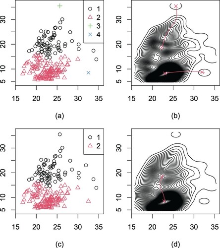
It can be seen from the histogram of the BMI in Figure 1 that the response is right-skewed, indicating the preference of the model with the skew-normal random errors. We determine the number of components via the method in Subsection 5.3. The clustering results are shown in Figure 2. At the level 3, 4 clusters are formed, as shown by different symbols in Figure 2(a). The 4 modes identified at level 3 are merged into 2 modes at level 4, as shown in Figure 2(b,d). Compared with level 4, two influential observations were excluded in cluster 1 and cluster 2 of level 3. Thus, it seems reasonable to use the following FMMeR model with two components to fit the BMI data, (20) $\{\begin{array}{rl}f(y_i\mid \mathbf{\Psi })& ={\nu }_{1}SN({\mu }_{i1},{\sigma }_1^2,{\lambda }_1)+(1-{\nu }_1)SN({\mu }_{i2},{\sigma }_2^2,{\lambda }_2),\\ \mathrm{M}\mathrm{e}\mathrm{d}\mathrm{i}\mathrm{a}\mathrm{n}\left(y_{ij}\right)& ={\mathit{x}}_i^{\mathrm{\top }}{\text{β}}_j,i=1,2,\dots ,202,j=1,2,\end{array}$(20) where ${\mu }_{i1}$ and ${\mu }_{i2}$ are defined by (9(9) ${\mu }_{ij}={\mathit{x}}_i^{\mathrm{\top }}{\text{β}}_j-\frac{{\sigma }_j}{3}\left[m_0\right({\lambda }_j)+2\sqrt{\frac{2}{\text{π}}}\delta ({\lambda }_j\left)\right],$(9) ), and $\mathbf{\Psi }=({\nu }_1,{\text{β}}_1^{\mathrm{\top }},{\text{β}}_2^{\mathrm{\top }},{\sigma }_1,{\sigma }_2,{\lambda }_1,{\lambda }_2{)}^{\mathrm{\top }}$. ${\mathit{x}}_i$ is a $10\times 1$ vector consisting of all 10 potential variables. Three penalty functions are used to select significant variables.

Figure 1. Histogram of the BMI.

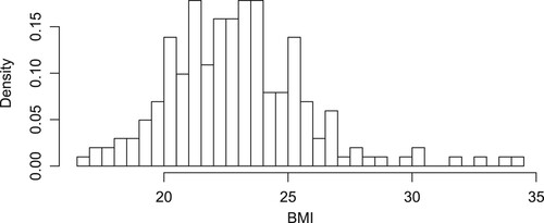
Figure 2. Clustering results for the BMI data obtained. (a) The 4 clusters at level 3. (b) The ascending paths from the modes at level 3 to those at level 4 and the contours of the density estimate at level 4. (c) The 2 clusters at level 4. (d) The ascending paths from the modes at level 4 to the next level and the contours of the density estimate at the next level.

We compare the variable selection results of the three models, including the proposed FMMeR model in this article, finite mixture of modal liner regression model and NMR model, where modal liner regression (MODLR) model was proposed by Yao and Li (2014). The results of variable selection for three models are given in Tables 5–7. In this data example, three variable selection procedures for a given model perform very similarly in terms of selecting significant variables. For FMMeR model and finite mixture of MODLR model, the same variables are removed for a given penalty function. NMR model, however, reserves more variables, resulting in a failure to select significant variables. Thus, the true structure of the model is not identified. When there is a situation of skewed data, the performances of HARD and SCAD are better than LASSO for identifying the authentic structure of the model. In FMMeR model, seven significant variables, including ${\mathit{x}}_1$, ${\mathit{x}}_4$, ${\mathit{x}}_5$, ${\mathit{x}}_7$, ${\mathit{x}}_8$, ${\mathit{x}}_9$, ${\mathit{x}}_{10}$, are identified in component 1. Also seven ${\mathit{x}}_4$, ${\mathit{x}}_5$, ${\mathit{x}}_6$, ${\mathit{x}}_7$, ${\mathit{x}}_8$, ${\mathit{x}}_9$, ${\mathit{x}}_{10}$ are contained in component 2. This indicates that these variables have a significant effect for BMI of athletes. We also find that there are some variables having different effects on parts one and two. For instance, red cell count $\left({\mathit{x}}_1\right)$ and sum of skin folds (${\mathit{x}}_6$) are another factors affecting athletes' BMI in component 1 and component 2, respectively. Furthermore, ${\mathit{x}}_4$, ${\mathit{x}}_5$, ${\mathit{x}}_7$ and ${\mathit{x}}_8$ are helpful for achieving a high BMI in two conponents. In addition, the performance of the variable selection procedure via the FMMeR model is different from that of the variable selection procedure via the NMR model.

Table 5. Variable selection for BMI data set via FMMeR model.

	LASSO		HARD		SCAD
Covariates	Com.1	Com.2	Com.1	Com.2	Com.1	Com.2
${\mathit{x}}_1$			−0.7386		−0.7224
${\mathit{x}}_2$		0.0674
${\mathit{x}}_3$
${\mathit{x}}_4$	0.8752	0.7071	1.0808	0.7490	1.0726	0.7358
${\mathit{x}}_5$	0.0032	0.0069	0.0027	0.0027	0.0034	0.0016
${\mathit{x}}_6$		0.0501		0.0468		0.0424
${\mathit{x}}_7$	0.2773	0.5750	0.7060	0.6165	0.6848	0.5997
${\mathit{x}}_8$	0.2087	1.1808	0.6887	1.1974	0.6666	1.1324
${\mathit{x}}_9$	−0.0446	−0.1054	−0.0668	−0.1067	−0.0656	−0.1003
${\mathit{x}}_{10}$		−0.7357	−0.4254	−0.7508	−0.4060	−0.7007

Table 6. Variable selection for BMI data set via finite mixture of MODLR model.

	LASSO		HARD		SCAD
Covariates	Com.1	Com.2	Com.1	Com.2	Com.1	Com.2
${\mathit{x}}_1$			−0.7244		−0.7226
${\mathit{x}}_2$		0.0709
${\mathit{x}}_3$
${\mathit{x}}_4$	0.8790	0.6873	1.0554	0.7283	1.0496	0.7153
${\mathit{x}}_5$	0.0038	0.0070	0.0033	0.0026	0.0032	0.0019
${\mathit{x}}_6$		0.0486		0.0447		0.0410
${\mathit{x}}_7$	0.2690	0.6033	0.7884	0.6480	0.7628	0.6284
${\mathit{x}}_8$	0.2062	1.2133	0.7931	1.2285	0.7621	1.1663
${\mathit{x}}_9$	−0.0454	−0.1079	−0.0714	−0.1089	−0.0687	−0.1027
${\mathit{x}}_{10}$		−0.7595	−0.5188	−0.7734	−0.4929	−0.7256

Table 7. Variable selection for BMI data set via NMR model.

	LASSO		HARD		SCAD
Covariates	Com.1	Com.2	Com.1	Com.2	Com.1	Com.2
${\mathit{x}}_1$	−0.9520		−0.9582
${\mathit{x}}_2$	−0.0457	0.0824	−0.0451	0.0824
${\mathit{x}}_3$	0.0754		0.0759
${\mathit{x}}_4$	0.9064	0.6228	0.9067	0.6227	0.0794	0.0693
${\mathit{x}}_5$	0.0049	0.0081	0.0049	0.0081	0.0003	0.0003
${\mathit{x}}_6$	−0.019	0.0438	−0.0189	0.0437		0.0038
${\mathit{x}}_7$	0.8690	0.6757	0.8703	0.6761	0.0244	0.0634
${\mathit{x}}_8$	0.7615	1.2918	0.7639	1.2921	0.0195	0.1164
${\mathit{x}}_9$	−0.0729	−0.1134	−0.0731	−0.1134	0.0068	0.0008
${\mathit{x}}_{10}$	−0.4855	−0.8169	−0.4876	−0.8172	−0.0137	−0.0884

8. Conclusions remarks and future works

In this paper, by utilizing the skew-normal distribution as a component density to overcome the potential inappropriateness of normal mixtures in some context, we have developed a novel finite mixture of the median regression (FMMeR) model to explore asymmetrical data that arise from several subpopulations. Thanks to the stochastic representation for the skew-normal distribution, we have constructed a hierarchical representation of the finite skew-normal mixtures to address computational barriers of the parameter estimation and variable selection when fitting the FMMeR model. In addition, in order to determine the number of components, we applied a clustering method via mode identification proposed by J. Li et al. (2007) and a good performance is shown. Numerical results from simulation studies and a real-data example illustrated that the proposed FMMeR model methodology performs well in general, even when the data exhibit symmetrical behaviour.

It is worth noting that we only considered the procedures of parameter estimation and variable selection for the FMMeR model based on a mixture of the skew-normal distributions. Meanwhile, the scenario of p>n has not been considered in this paper. A natural extension of the proposed methodology is to consider other skewed distributions, such as the skew-t and skew-Laplace distributions, and high-dimensional settings. In addition, another research direction is to model the mixing proportions $\mathit{\nu }$, which extends the proposed model to the framework of mixture of experts models. Finally, it will also be of interest to consider Bayesian variable selection, semi-parametric and nonparametric methods for the FMMeR model, which are currently under investigation and will be reported elsewhere.

Disclosure statement

No potential conflict of interest was reported by the author(s).

Additional information

Funding

This work is partially supported by the National Natural Science Foundation of China [grant number 11861041], the Natural Science Research Foundation of Kunming University of Science and Technology [grant number KKSY201907003].

Appendices

Appendix 1. Regularity conditions and proofs

Regularity conditions $R_1\text{--}{R}_4$ on the joint distribution of $h=(\mathit{x},Y)$ are needed for proving the asymptotic properties of the proposed method. Let $f(h\mid \mathbf{\Psi })$ be the joint density function of h with the parameter space $\mathbf{\Psi }\in \mathbf{\Omega }$. We write $\mathbf{\Psi }=({\psi }_1,{\psi }_2,\dots ,{\psi }_s)$ and s is the total number of parameters in the FMMeR model. The regularity conditions are as follows.

R1:	The density $f(h\mid \mathbf{\Psi })$ has common support in h for all $\mathbf{\Psi }\in \mathbf{\Omega }$, and $f(h\mid \mathbf{\Psi })$ is identifiable in $\mathbf{\Psi }$ up to a permutation of the components of the mixture.
R2:	There exists an open subset ${\mathbf{\Omega }}^{\ast }\in \mathbf{\Omega }$ containing the true parameter ${\mathbf{\Psi }}_0$ such that for almost all h, the density $f(h\mid \mathbf{\Psi })$ admits third partial derivatives with respect to $\mathbf{\Psi }\in {\mathbf{\Omega }}^{\ast }$.
R3:	For each ${\mathbf{\Psi }}_0\in \mathbf{\Psi }$ and $t,l,g=1,2,\dots ,s$, there exist functions $B_1\left(h\right)$ and $B_2\left(h\right)$ (possibly depending on ${\mathbf{\Psi }}_0$) such that for $\mathbf{\Psi }$ in a neighbourhood of $N\left({\mathbf{\Psi }}_0\right)$, $\begin{array}{rl}\left|\frac{\mathrm{\partial }f(h\mid \mathbf{\Psi })}{\mathrm{\partial }{\psi }_t}\right|\le B_1\left(h\right),\left|\frac{{\mathrm{\partial }}^{2}f(h\mid \mathbf{\Psi })}{\mathrm{\partial }{\psi }_t\mathrm{\partial }{\psi }_l}\right|\le B_1\left(h\right),\left|\frac{{\mathrm{\partial }}^3\log f(h\mid \mathbf{\Psi })}{\mathrm{\partial }{\psi }_t\mathrm{\partial }{\psi }_l\mathrm{\partial }{\psi }_g}\right|& \le B_2\left(h\right),\end{array}$ where $\int B_1\left(h\right)\mathrm{d}h<\mathrm{\infty }$ and $\int B_2\left(h\right)f(h\mid \mathbf{\Psi })\mathrm{d}h<\mathrm{\infty }$.
R4:	The Fisher information matrix, $I\left(\mathbf{\Psi }\right)=E\left\{[\frac{\mathrm{\partial }}{\mathrm{\partial }\mathbf{\Psi }}\log f(h\mid \mathbf{\Psi }\left)\right]{[\frac{\mathrm{\partial }}{\mathrm{\partial }\mathbf{\Psi }}\log f(h\mid \mathbf{\Psi }\left)\right]}^{\mathrm{\top }}\right\},$is finite and positive definite for each $\mathbf{\Psi }\in \mathbf{\Omega }$.

Proof

Proof of Theorem 4.1

Let ${\xi }_n=n^{-1/2}(1+a_n)$. We just have to specify that for any given $ϵ>0$, there exists a large constant C such that (A1) $\underset{n\to \mathrm{\infty }}{lim}P\left\{\underset{\Vert \mathit{u}\Vert =C}{sup}L\right({\mathbf{\Psi }}_0+{\xi }_n\mathit{u})<L({\mathbf{\Psi }}_0\left)\right\}\ge 1-ϵ.$(A1) This indicates that for sufficiently large n, with large probability namely $1-ϵ$, there is a localmaximum in the ball $\{{\mathbf{\Psi }}_0+{\xi }_n\mathit{u}:\Vert \mathit{u}\Vert \le C\}$. This localmaximizer, say $\hat{\mathbf{\Psi }}$, satisfies $\Vert \hat{\mathbf{\Psi }}-{\mathbf{\Psi }}_0\Vert =O_p\left({\xi }_n\right)$.

Let ${\zeta }_n\left(\mathit{u}\right)=L({\mathbf{\Psi }}_0+{\xi }_n\mathit{u})-L\left({\mathbf{\Psi }}_0\right)$. Using $p_{{\tau }_j}\left(0\right)=0$ and the definition of $L(\cdot )$, we have $\begin{array}{rl}{\zeta }_n\left(\mathit{u}\right)& =\left[\ell \right({\mathbf{\Psi }}_0+{\xi }_n\mathit{u})-\ell ({\mathbf{\Psi }}_0\left)\right]-\left[p\right({\mathbf{\Psi }}_0+{\xi }_n\mathit{u})-p({\mathbf{\Psi }}_0\left)\right]\\ & \le \left[\ell \right({\mathbf{\Psi }}_0+{\xi }_n\mathit{u})-\ell ({\mathbf{\Psi }}_0\left)\right]-\left[p\right({\mathbf{\Psi }}_{01}+{\xi }_n{\mathit{u}}_{\mathit{I}})-p({\mathbf{\Psi }}_{01}\left)\right]\\ & \le \ell ({\mathbf{\Psi }}_0+{\xi }_n\mathit{u})-\ell \left({\mathbf{\Psi }}_0\right)-n\sum _{j=1}^m{\nu }_j\sum _{t=1}^{d_j}\left[p_{{\tau }_j}\right({\text{β}}_{jt}^0+{\xi }_n{\mathit{u}}_{\mathit{I}})-p_{{\tau }_j}({\text{β}}_{jt}^0\left)\right],\end{array}$where $d_j$ is the number of nonzero elements of the vector ${\text{β}}_j^0$. ${\mathbf{\Psi }}_{01}$ is the parameter vector with zero regression coefficients removed and ${\mathit{u}}_{\mathit{I}}$ is a subvector of $\mathit{u}$ with corresponding components. By Taylor's expansion and the triangular inequality (A2) $\begin{array}{rl}{\zeta }_n\left(\mathit{u}\right)& \le {\xi }_n\left\{\ell \right({\mathbf{\Psi }}_0^{\mathrm{\prime }}){\}}^{\mathrm{\top }}\mathit{u}-\frac{1}{2}{\mathit{u}}^{\mathrm{\top }}I({\mathbf{\Psi }}_0\left)\mathit{u}n{\xi }_n^2\right\{1+o_p\left(1\right)\}\\ & -\sum _{j=1}^m{\nu }_j\sum _{t=1}^{d_j}\left[n{\xi }_n{p}_{{\tau }_j}^{\mathrm{\prime }}\right({\text{β}}_{jt}^0){\mathit{u}}_{\mathit{I}}+n{\xi }_n^2{p}_{{\tau }_j}^{\mathrm{\prime }\mathrm{\prime }}{\mathit{u}}_{\mathit{I}}^2\{1+o\left(1\right)\left\}\right]\\ & =q_1+q_2+q_3.\end{array}$(A2) Regularity conditions imply that $n^{-1/2}{\ell }^{\mathrm{\prime }}\left({\mathbf{\Psi }}_0\right)=O_p\left(1\right)$ and Fisher informationmatrix $I\left({\mathbf{\Psi }}_0\right)$ is positive definite. Thus, $q_1$ is of the order $O_p\left(n^{1/2}{\xi }_n\right)=O_p\left(n{\xi }_n^2\right)$. By choosing a sufficiently large C, $q_1$ is controlled uniformly by $q_2$ in $\Vert \mathit{u}\Vert =C$. Note that the $q_3$ is bounded by $\begin{array}{rl}& \sum _{j=1}^m{\nu }_j\{\sqrt{d}n{\xi }_n{a}_n\Vert \mathit{u}\Vert +n{\xi }_n^2{b}_n\Vert \mathit{u}{\Vert }^2\}=\sqrt{d}n{\xi }_n{a}_n\Vert \mathit{u}\Vert +n{\xi }_n^2{b}_n\Vert \mathit{u}{\Vert }^2,\end{array}$where $d=\underset{j}{max}{d}_j$. By condition $C_1$ for the penalty functions, $b_n=o\left(1\right)$, this is also dominated by the $q_2$. Hence, by choosing a sufficiently large C, (A1(A1) $\underset{n\to \mathrm{\infty }}{lim}P\left\{\underset{\Vert \mathit{u}\Vert =C}{sup}L\right({\mathbf{\Psi }}_0+{\xi }_n\mathit{u})<L({\mathbf{\Psi }}_0\left)\right\}\ge 1-ϵ.$(A1) ) holds. This completes the proof.

Proof

Proof of Theorem 4.2

To prove part (a), consider the partition $\mathbf{\Psi }=({\mathbf{\Psi }}_1,{\mathbf{\Psi }}_2)$ for any $\mathbf{\Psi }$ in the neighbourhood $\Vert \mathbf{\Psi }-{\mathbf{\Psi }}_0\Vert =O\left(n^{-1/2}\right)$. By the definition of $L(\cdot )$, we obtain $\begin{array}{r}L({\mathbf{\Psi }}_1,{\mathbf{\Psi }}_2)-L({\mathbf{\Psi }}_1,\mathbf{0})=\left[\ell \right({\mathbf{\Psi }}_1,{\mathbf{\Psi }}_2)-\ell ({\mathbf{\Psi }}_1,\mathbf{0}\left)\right]-\left[p\right({\mathbf{\Psi }}_1,{\mathbf{\Psi }}_2)-p({\mathbf{\Psi }}_1,\mathbf{0}\left)\right].\end{array}$By the mean value theorem, (A3) $\ell ({\mathbf{\Psi }}_1,{\mathbf{\Psi }}_2)-\ell ({\mathbf{\Psi }}_1,\mathbf{0})={\left[\frac{\mathrm{\partial }\ell ({\mathbf{\Psi }}_1,\mathit{\eta })}{\mathrm{\partial }{\mathbf{\Psi }}_2}\right]}^{\mathrm{\top }}{\mathbf{\Psi }}_2$(A3) with $\Vert \mathit{\eta }\Vert \le \Vert {\mathbf{\Psi }}_2\Vert =O\left(n^{-1/2}\right)$. Furthermore, by using regularity condition $R_3$ and the mean value theorem, we have $\begin{array}{rl}\Vert \frac{\mathrm{\partial }\ell ({\mathbf{\Psi }}_1,\mathit{\eta })}{\mathrm{\partial }{\mathbf{\Psi }}_2}-\frac{\mathrm{\partial }\ell ({\mathbf{\Psi }}_{01},\mathbf{0})}{\mathrm{\partial }{\mathbf{\Psi }}_2}\Vert & \le \Vert \frac{\mathrm{\partial }\ell ({\mathbf{\Psi }}_1,\mathit{\eta })}{\mathrm{\partial }{\mathbf{\Psi }}_2}-\frac{\mathrm{\partial }\ell ({\mathbf{\Psi }}_1,\mathbf{0})}{\mathrm{\partial }{\mathbf{\Psi }}_2}\Vert +\Vert \frac{\mathrm{\partial }\ell ({\mathbf{\Psi }}_1,\mathbf{0})}{\mathrm{\partial }{\mathbf{\Psi }}_2}-\frac{\mathrm{\partial }\ell ({\mathbf{\Psi }}_{01},\mathbf{0})}{\mathrm{\partial }{\mathbf{\Psi }}_2}\Vert \\ & \le \left[\sum _{i=1}^n{B}_1\right(h_i\left)\right]\Vert \mathit{\eta }\Vert +\left[\sum _{i=1}^n{B}_1\right(h_i\left)\right]\Vert {\mathbf{\Psi }}_1-{\mathbf{\Psi }}_{01}\Vert \\ & =\{\Vert \mathit{\eta }\Vert +\Vert {\mathbf{\Psi }}_1-{\mathbf{\Psi }}_{01}\Vert \}{O}_p\left(n\right)=O_p\left(n^{1/2}\right).\end{array}$By the regularity conditions $R_1$–$R_4$, $\mathrm{\partial }\ell ({\mathbf{\Psi }}_{01},\mathbf{0})/\mathrm{\partial }{\mathbf{\Psi }}_2=O_p\left(n^{1/2}\right)$. Thus, $\mathrm{\partial }\ell ({\mathbf{\Psi }}_1,\mathit{\eta })/\mathrm{\partial }{\mathbf{\Psi }}_2=O_p\left(n^{1/2}\right)$. Applying these order assessments to (A3(A3) $\ell ({\mathbf{\Psi }}_1,{\mathbf{\Psi }}_2)-\ell ({\mathbf{\Psi }}_1,\mathbf{0})={\left[\frac{\mathrm{\partial }\ell ({\mathbf{\Psi }}_1,\mathit{\eta })}{\mathrm{\partial }{\mathbf{\Psi }}_2}\right]}^{\mathrm{\top }}{\mathbf{\Psi }}_2$(A3) ), we obtain $\ell ({\mathbf{\Psi }}_1,{\mathbf{\Psi }}_2)-\ell ({\mathbf{\Psi }}_1,\mathbf{0})=O_p\left(n^{1/2}\right)\sum _{j=1}^m\sum _{t=d_j+1}^p|{\text{β}}_{jt}|,$for large n. On the other hand, $p({\mathbf{\Psi }}_1,{\mathbf{\Psi }}_2)-p({\mathbf{\Psi }}_1,\mathbf{0})=n\sum _{j=1}^m\sum _{t=d_j+1}^p{\nu }_j{p}_{{\tau }_j}\left({\text{β}}_{jt}\right).$Thus, $\begin{array}{r}L({\mathbf{\Psi }}_1,{\mathbf{\Psi }}_2)-L({\mathbf{\Psi }}_1,\mathbf{0})=\sum _{j=1}^m\sum _{t=d_j+1}^p\left\{|{\text{β}}_{jt}|O_p\right(n^{1/2})-n{\nu }_j{p}_{{\tau }_j}({\text{β}}_{jt}\left)\right\}.\end{array}$In a shrinking neighbourhood of 0, $|{\text{β}}_{jt}|O_p\left(n^{1/2}\right)<n{\nu }_j{p}_{{\tau }_j}\left({\text{β}}_{jt}\right)$ in probability by condition $C_2$. This completes the proof of part (a).

To prove sparsity in part (b(1)), we consider the partition $\mathbf{\Psi }=L({\mathbf{\Psi }}_1,{\mathbf{\Psi }}_2)$. Let $({\hat{\mathbf{\Psi }}}_1,\mathbf{0})$ be the maximizer of the penalized log-likelihood function $L(\mathbf{\Psi },\mathbf{0})$, which is considered as a function of ${\mathbf{\Psi }}_1$. It suffices to show that in the neighbourhood $\Vert \mathbf{\Psi }-{\mathbf{\Psi }}_0\Vert =O_p\left\{n^{-1/2}\right\}$, $L({\mathbf{\Psi }}_1,{\mathbf{\Psi }}_2)-L({\hat{\mathbf{\Psi }}}_1,\mathbf{0})<0$ with probability tending to 1 as $n\to \mathrm{\infty }$. By the result in part (a), we obtain that $\begin{array}{rl}L({\mathbf{\Psi }}_1,{\mathbf{\Psi }}_2)-L({\hat{\mathbf{\Psi }}}_1,\mathbf{0})& =\left[L\right({\mathbf{\Psi }}_1,{\mathbf{\Psi }}_2)-L({\mathbf{\Psi }}_1,\mathbf{0}\left)\right]+\left[L\right({\mathbf{\Psi }}_1,\mathbf{0})-L({\hat{\mathbf{\Psi }}}_1,\mathbf{0}\left)\right]\\ & \le \left[L\right({\mathbf{\Psi }}_1,{\mathbf{\Psi }}_2)-L({\mathbf{\Psi }}_1,\mathbf{0}\left)\right]<0.\end{array}$To prove asymptotic normality in part (b(2)), we consider $L(\mathbf{\Psi },\mathbf{0})$ as a function of ${\mathbf{\Psi }}_1$. Using the same argument as in Theorem 4.1, there exists a $\sqrt{n}$-consistent local maximizer of this function, denoted by ${\hat{\mathbf{\Psi }}}_1$, that satisfies $\frac{\mathrm{\partial }L\left(\hat{\mathbf{\Psi }}\right)}{\mathrm{\partial }{\mathbf{\Psi }}_1}={\{\frac{\mathrm{\partial }\ell \left(\mathbf{\Psi }\right)}{\mathrm{\partial }{\mathbf{\Psi }}_1}-\frac{\mathrm{\partial }p\left(\mathbf{\Psi }\right)}{\mathrm{\partial }{\mathbf{\Psi }}_1}\}}_{\hat{\mathbf{\Psi }}=({\hat{\mathbf{\Psi }}}_1,\mathbf{0})}=\mathbf{0}.$By substituting the first-order Taylor's expansions of $\mathrm{\partial }\ell \left(\mathbf{\Psi }\right)/\mathrm{\partial }{\mathbf{\Psi }}_1$ and $\mathrm{\partial }p\left(\mathbf{\Psi }\right)/\mathrm{\partial }{\mathbf{\Psi }}_1$ into the above expression, we have $\begin{array}{r}\{\frac{{\mathrm{\partial }}^2\ell \left({\mathbf{\Psi }}_{01}\right)}{\mathrm{\partial }{\mathbf{\Psi }}_1\mathrm{\partial }{\mathbf{\Psi }}_1^{\mathrm{\top }}}-p^{\mathrm{\prime }\mathrm{\prime }}({\mathbf{\Psi }}_{01})+o_p(n\left)\right\}({\hat{\mathbf{\Psi }}}_1-{\mathbf{\Psi }}_{01})=\frac{\mathrm{\partial }\ell \left({\mathbf{\Psi }}_{01}\right)}{\mathrm{\partial }{\mathbf{\Psi }}_1}-p^{\mathrm{\prime }}\left({\mathbf{\Psi }}_{01}\right).\end{array}$On the other hand, under the regularity conditions, we obtain $\frac{{\mathrm{\partial }}^2\ell \left({\mathbf{\Psi }}_{01}\right)}{\mathrm{\partial }{\mathbf{\Psi }}_1\mathrm{\partial }{\mathbf{\Psi }}_1^{\mathrm{\top }}}=I_1\left({\mathbf{\Psi }}_{01}\right)+o_p\left(1\right),$and $\frac{1}{\sqrt{n}}\frac{\mathrm{\partial }\ell \left({\mathbf{\Psi }}_{01}\right)}{\mathrm{\partial }{\mathbf{\Psi }}_1}⟹dN(\mathbf{0},I_1({\mathbf{\Psi }}_{01}\left)\right).$Using the foregoing facts and Slutsky's theorem, we have $\begin{array}{r}\sqrt{n}\left\{\left[I_1\right({\mathbf{\Psi }}_{01})-\frac{p^{\mathrm{\prime }\mathrm{\prime }}\left({\mathbf{\Psi }}_{01}\right)}{n}]\right({\hat{\mathbf{\Psi }}}_1-{\mathbf{\Psi }}_{01})+\frac{p^{\mathrm{\prime }}\left({\mathbf{\Psi }}_{01}\right)}{n}\}⟹dN(\mathbf{0},I_1({\mathbf{\Psi }}_{01}\left)\right),\end{array}$which is the result in part (b(2)).

Appendix 2. Some technical derivations

In (5.9), the score function of j-th component is expressed as $\begin{array}{rl}S\left({\text{β}}_j\right)& =-\sum _{i=1}^n{\omega }_{ij}^{\left(k\right)}\frac{(1+{\lambda }_j^2)}{{\sigma }_j^2}(e_{ij}{\mathit{E}}_1-{\sigma }_j{r}_{1i}^{\left(k\right)}\delta ({\lambda }_j\left){\mathit{E}}_1\right),\\ S\left({\sigma }_j\right)& =-\frac{1}{{\sigma }_j}\sum _{i=1}^n{\omega }_{ij}^{\left(k\right)}+\frac{(1+{\lambda }_j^2)}{{\sigma }_j^2}\sum _{i=1}^n{\omega }_{ij}^{\left(k\right)}\left[\frac{e_{ij}^2}{{\sigma }_j}-e_{ij}{r}_{1i}^{\left(k\right)}\delta \right({\lambda }_j)\\ & \phantom{\frac{e_{ij}^2}{{\sigma }_j}}-e_{ij}{E}_2+{\sigma }_j{r}_{1i}^{\left(k\right)}\delta \left({\lambda }_j\right)E_2],\\ S\left({\lambda }_j\right)& =\sum _{i=1}^n{\omega }_{ij}^{\left(k\right)}\frac{{\delta }^2\left({\lambda }_j\right)}{{\lambda }_j}-\sum _{i=1}^n{\omega }_{ij}^{\left(k\right)}[\frac{e_{ij}^2{\lambda }_j}{{\sigma }_j^2}+\frac{e_{ij}(1+{\lambda }_j^2)}{{\sigma }_j^2}{E}_3\\ & -\frac{r_{1i}^{\left(k\right)}}{{\sigma }_j}\left(\frac{e_{ij}\delta \left({\lambda }_j\right)}{{\lambda }_j}+2e_{ij}{\lambda }_j\delta \right({\lambda }_j\left)+\frac{{\lambda }_j^2}{\delta \left({\lambda }_j\right)}{E}_3\right)+{\lambda }_j{r}_{2i}^{\left(k\right)}].\end{array}$ $H\left(\mathit{\theta }\right)$ is defined as $\begin{array}{r}H\left(\mathit{\theta }\right)=\frac{{\mathrm{\partial }}^2{Q}_2(\mathit{\theta };{\mathbf{\Psi }}^{\left(k\right)})}{\mathrm{\partial }\mathit{\theta }\mathrm{\partial }{\mathit{\theta }}^{\mathrm{\top }}}=\left[\begin{array}{ccc}{\displaystyle \frac{{\mathrm{\partial }}^2{Q}_2(\mathit{\theta };{\mathbf{\Psi }}^{\left(k\right)})}{\mathrm{\partial }{\text{β}}_j\mathrm{\partial }{\text{β}}_j^{\mathrm{\top }}}}& {\displaystyle \frac{{\mathrm{\partial }}^2{Q}_2(\mathit{\theta };{\mathbf{\Psi }}^{\left(k\right)})}{\mathrm{\partial }{\text{β}}_j\mathrm{\partial }{\sigma }_j}}& {\displaystyle \frac{{\mathrm{\partial }}^2{Q}_2(\mathit{\theta };{\mathbf{\Psi }}^{\left(k\right)})}{\mathrm{\partial }{\text{β}}_j\mathrm{\partial }{\lambda }_j}}\\ \ast & {\displaystyle \frac{{\mathrm{\partial }}^2{Q}_2(\mathit{\theta };{\mathbf{\Psi }}^{\left(k\right)})}{\mathrm{\partial }{\sigma }_j\mathrm{\partial }{\sigma }_j}}& {\displaystyle \frac{{\mathrm{\partial }}^2{Q}_2(\mathit{\theta };{\mathbf{\Psi }}^{\left(k\right)})}{\mathrm{\partial }{\sigma }_j\mathrm{\partial }{\lambda }_j}}\\ \ast & \ast & {\displaystyle \frac{{\mathrm{\partial }}^2{Q}_2(\mathit{\theta };{\mathbf{\Psi }}^{\left(k\right)})}{\mathrm{\partial }{\lambda }_j\mathrm{\partial }{\lambda }_j}}\end{array}\right],\end{array}$where $\begin{array}{rl}\frac{{\mathrm{\partial }}^2{Q}_2(\mathit{\theta };{\mathbf{\Psi }}^{\left(k\right)})}{\mathrm{\partial }{\text{β}}_j\mathrm{\partial }{\text{β}}_j^{\mathrm{\top }}}& =\sum _{i=1}^n{\omega }_{ij}^{\left(k\right)}\frac{(1+{\lambda }_j^2)}{{\sigma }_j^2}{\mathit{E}}_1{\mathit{E}}_1^{\mathrm{\top }},\\ \frac{{\mathrm{\partial }}^2{Q}_2(\mathit{\theta };{\mathbf{\Psi }}^{\left(k\right)})}{\mathrm{\partial }{\text{β}}_j\mathrm{\partial }{\sigma }_j}& =\sum _{i=1}^n{\omega }_{ij}^{\left(k\right)}\frac{(1+{\lambda }_j^2)}{{\sigma }_j^2}\left[\right(\delta \left({\lambda }_j\right)+2e_{ij}-2{\sigma }_j{r}_{1i}^{\left(k\right)}\delta \left({\lambda }_j\right)]{\mathit{E}}_1,\\ \frac{{\mathrm{\partial }}^2{Q}_2(\mathit{\theta };{\mathbf{\Psi }}^{\left(k\right)})}{\mathrm{\partial }{\text{β}}_j\mathrm{\partial }{\lambda }_j}& =-\sum _{i=1}^n{\omega }_{ij}^{\left(k\right)}[\frac{2{\lambda }_j{e}_{ij}+(1+{\lambda }_j^2)E_3}{{\sigma }_j^2}+\frac{r_{1i}^{\left(k\right)}}{{\sigma }_j}\left[2{\lambda }_j\delta \right({\lambda }_j)+\frac{\delta \left({\lambda }_j\right)}{{\lambda }_j}]{\mathit{E}}_1],\\ \frac{{\mathrm{\partial }}^2{Q}_2(\mathit{\theta };{\mathbf{\Psi }}^{\left(k\right)})}{\mathrm{\partial }{\sigma }_j\mathrm{\partial }{\sigma }_j}& =\frac{1}{{\sigma }_j^2}\sum _{i=1}^n{\omega }_{ij}^{\left(k\right)}+\sum _{i=1}^n{\omega }_{ij}^{\left(k\right)}\frac{(1+{\lambda }_j^2)}{{\sigma }_j^2}[\frac{2e_{ij}(2E_2+r_{1i}^{\left(k\right)}\delta ({\lambda }_j\left)\right)}{{\sigma }_j}-\frac{3e_{ij}^2}{{\sigma }_j^2}\\ & -2r_{1i}^{\left(k\right)}\delta \left({\lambda }_j\right)E_2-e_{ij}{E}_{22}+{\sigma }_j\delta \left({\lambda }_j\right)r_{1i}^{\left(k\right)}{E}_{22}-E_2^2\phantom{\frac{2e_{ij}(2E_2+r_{1i}^{\left(k\right)}\delta ({\lambda }_j\left)\right)}{{\sigma }_j}-\frac{3e_{ij}^2}{{\sigma }_j^2}}],\\ \frac{{\mathrm{\partial }}^2{Q}_2(\mathit{\theta };{\mathbf{\Psi }}^{\left(k\right)})}{\mathrm{\partial }{\sigma }_j\mathrm{\partial }{\lambda }_j}& =\sum _{i=1}^n{\omega }_{ij}^{\left(k\right)}\frac{2{\lambda }_j{e}_{ij}}{{\sigma }_j^2}[\frac{e_{ij}}{{\sigma }_j}-r_{1i}^{\left(k\right)}\delta ({\lambda }_j)+\frac{{\sigma }_j{r}_{1i}^{\left(k\right)}\delta \left({\lambda }_j\right)E_2}{e_{ij}}-\frac{r_{1i}^{\left(k\right)}\delta \left({\lambda }_j\right)}{2{\lambda }_j^2}-E_2]\\ & -\sum _{i=1}^n{\omega }_{ij}^{\left(k\right)}\frac{(1+{\lambda }_j^2)}{{\sigma }_j^2}\left[r_{1i}^{\left(k\right)}\delta \right({\lambda }_j)+\frac{e_{ij}{E}_{23}}{E_3}-\frac{2e_{ij}{E}_3}{{\sigma }_j}+E_2],\\ \frac{{\mathrm{\partial }}^2{Q}_2(\mathit{\theta };{\mathbf{\Psi }}^{\left(k\right)})}{\mathrm{\partial }{\lambda }_j\mathrm{\partial }{\lambda }_j}& =\sum _{i=1}^n{\omega }_{ij}^{\left(k\right)}\frac{1-{\lambda }_j^2}{(1+{\lambda }_j^2{)}^2}-\sum _{i=1}^n{\omega }_{ij}^{\left(k\right)}\left[\phantom{\frac{(1+{\lambda }_j^2)}{{\sigma }_j^2}}\frac{e_{ij}}{{\sigma }_j^2}\right(e_{ij}+4{\lambda }_j{E}_3)+\frac{(1+{\lambda }_j^2)}{{\sigma }_j^2}(E_3^2+e_{ij}{E}_{33})\\ & -\frac{r_{1i}^{\left(k\right)}}{{\sigma }_j}(\frac{e_{ij}\delta \left({\lambda }_j\right)}{1+{\lambda }_j^2}+2\delta ({\lambda }_j\left)\right(e_{ij}+{\lambda }_j{E}_3)+\sqrt{1+{\lambda }_j^2}({\lambda }_j{E}_{33}+2E_3\left)\phantom{\frac{e_{ij}\delta \left({\lambda }_j\right)}{1+{\lambda }_j^2}}\right)+r_{2i}^{\left(k\right)}],\end{array}$with $e_{ij}=y_i-{\mathit{x}}_i^{\mathrm{\top }}{\text{β}}_j-\frac{{\sigma }_j}{3}\left[m_0\right({\lambda }_j)+2\sqrt{\frac{2}{\text{π}}}\delta ({\lambda }_j\left)\right]$. Thus, we have $\{\begin{array}{rl}& {\mathit{E}}_1=\frac{\mathrm{\partial }{e}_{ij}}{\mathrm{\partial }{\text{β}}_j}=-{\mathit{x}}_i,\\ & E_2=\frac{\mathrm{\partial }{e}_{ij}}{\mathrm{\partial }{\sigma }_j}=\frac{1}{3}\left[m_0\right({\lambda }_j)+2\sqrt{\frac{2}{\text{π}}}\delta ({\lambda }_j\left)\right],\\ & E_3=\frac{\mathrm{\partial }{e}_{ij}}{\mathrm{\partial }{\lambda }_j}=\frac{{\sigma }_j}{3}[M_1+\sqrt{\frac{2}{\text{π}}}\frac{2}{(1+{\lambda }_j^2{)}^{3/2}}],\\ & {\mathit{E}}_{11}=\frac{{\mathrm{\partial }}^2{e}_{ij}}{\mathrm{\partial }{\text{β}}_j\mathrm{\partial }{\text{β}}_j^{\mathrm{\top }}}=\mathbf{0},\\ & E_{12}=E_{21}=\frac{{\mathrm{\partial }}^2{e}_{ij}}{\mathrm{\partial }{\text{β}}_j\mathrm{\partial }{\sigma }_j}=\frac{{\mathrm{\partial }}^2{e}_{ij}}{\mathrm{\partial }{\sigma }_j\mathrm{\partial }{\text{β}}_j^{\mathrm{\top }}}=0,\\ & E_{13}=E_{31}=\frac{{\mathrm{\partial }}^2{e}_{ij}}{\mathrm{\partial }{\text{β}}_j\mathrm{\partial }{\lambda }_j}=\frac{{\mathrm{\partial }}^2{e}_{ij}}{\mathrm{\partial }{\lambda }_j\mathrm{\partial }{\text{β}}_j^{\mathrm{\top }}}=0,\\ & E_{22}=\frac{{\mathrm{\partial }}^2{e}_{ij}}{\mathrm{\partial }{\sigma }_j\mathrm{\partial }{\sigma }_j}=0,\\ & E_{23}=E_{32}=\frac{{\mathrm{\partial }}^2{e}_{ij}}{\mathrm{\partial }{\sigma }_j\mathrm{\partial }{\sigma }_j}=\frac{1}{3}[M_1+\sqrt{\frac{2}{\text{π}}}\frac{2}{(1+{\lambda }_j^2{)}^{3/2}}],\\ & E_{33}=\frac{{\mathrm{\partial }}^2{e}_{ij}}{\mathrm{\partial }{\lambda }_j\mathrm{\partial }{\lambda }_j}=\frac{{\sigma }_j}{3}[M_2-\sqrt{\frac{2}{\text{π}}}\frac{6{\lambda }_j}{(1+{\lambda }_j^2{)}^{5/2}}],\end{array}$and $\begin{array}{rl}{M}_1=\frac{\mathrm{\partial }{m}_0\left({\lambda }_j\right)}{\mathrm{\partial }{\lambda }_j}& =\sqrt{\frac{2}{\text{π}}}\frac{1}{(1+{\lambda }_j^2{)}^{3/2}}-\frac{T_1{\sigma }_0\left({\lambda }_j\right)+S_1{t}_0\left({\lambda }_j\right)}{2}-\frac{\text{π}{\mathrm{s}\mathrm{i}\mathrm{g}\mathrm{n}}^2\left({\lambda }_j\right)}{{\lambda }_j^2}\exp (-\frac{2\text{π}}{|{\lambda }_j|}),\\ M_2=\frac{{\mathrm{\partial }}^2{m}_0\left({\lambda }_j\right)}{\mathrm{\partial }{\lambda }_j\mathrm{\partial }{\lambda }_j}& =-\sqrt{\frac{2}{\text{π}}}-\frac{3{\lambda }_j}{(1+{\lambda }_j^2{)}^{5/2}}-\frac{T_2{\sigma }_0\left({\lambda }_j\right)+2T_1{S}_1+S_2{t}_0\left({\lambda }_j\right)}{2}\\ & -\frac{2\text{π}\left[\text{π}\mathrm{s}\mathrm{i}\mathrm{g}\mathrm{n}\right({\lambda }_j)-{\lambda }_j{\mathrm{s}\mathrm{i}\mathrm{g}\mathrm{n}}^2({\lambda }_j\left)\right]}{{\lambda }_j^4}\exp (-\frac{2\text{π}}{|{\lambda }_j|}),\\ S_1& =\frac{\mathrm{\partial }{\sigma }_0\left({\lambda }_j\right)}{\mathrm{\partial }{\lambda }_j}=-\sqrt{\frac{2}{\text{π}}}\frac{{\mu }_0\left({\lambda }_j\right)}{{\sigma }_0\left({\lambda }_j\right)(1+{\lambda }_j^2{)}^{3/2}},\\ S_2& =\frac{{\mathrm{\partial }}^2{\sigma }_0\left({\lambda }_j\right)}{\mathrm{\partial }{\lambda }_j\mathrm{\partial }{\lambda }_j}=\frac{1}{{\sigma }_0\left({\lambda }_j\right)(1+{\lambda }_j^2{)}^3}\left[3{\lambda }_j{\mu }_0\right({\lambda }_j)\sqrt{1+{\lambda }_j^2}-\frac{2}{\text{π}{\sigma }_0\left({\lambda }_j\right)}],\\ T_1& =\frac{\mathrm{\partial }{t}_0\left({\lambda }_j\right)}{\mathrm{\partial }{\lambda }_j}=\frac{3(4-\text{π})}{2{\sigma }_0^4\left({\lambda }_j\right)}[\sqrt{\frac{2}{\text{π}}}\frac{{\mu }_0^2\left({\lambda }_j\right){\sigma }_0\left({\lambda }_j\right)}{(1+{\lambda }_j^2{)}^{3/2}}-{\mu }_0^3({\lambda }_j\left)S_1\right],\\ T_2& =\frac{{\mathrm{\partial }}^2{t}_0\left({\lambda }_j\right)}{\mathrm{\partial }{\lambda }_j\mathrm{\partial }{\lambda }_j}=\frac{3(4-\text{π})}{2{\sigma }_0^5\left({\lambda }_j\right)}[\frac{4{\mu }_0\left({\lambda }_j\right){\sigma }_0^2\left({\lambda }_j\right)}{\text{π}(1+{\lambda }_j^2{)}^{3/2}}-\sqrt{\frac{2}{\text{π}}}\frac{3{\lambda }_j{\mu }_0^2\left({\lambda }_j\right){\sigma }_0^2\left({\lambda }_j\right)}{(1+{\lambda }_j^2{)}^{5/2}}\\ & -\sqrt{\frac{2}{\text{π}}}\frac{6{\mu }_0^2\left({\lambda }_j\right){\sigma }_0\left({\lambda }_j\right)S_1}{(1+{\lambda }_j^2{)}^{3/2}}-S_2{\mu }_0^3\left({\lambda }_j\right){\sigma }_0\left({\lambda }_j\right)+4{\mu }_0^3\left({\lambda }_j\right)S_1^2].\end{array}$

References

- Akaike, H. (1973). Information theory and an extension of the maximum likelihood principle. International Symposium on Information Theory, 1, 610–624. https://doi.org/10.1007/978-1-4612-1694-0_15
- Atienza, N., Garcia-Heras, J., & Muñoz-Pichardo, J. (2006). A new condition for identifiability of finite mixture distributions. Metrika, 63(2), 215–221. https://doi.org/10.1007/s00184-005-0013-z
- Azzalini, A. (1985). A class of distributions which includes the normal ones. Scandinavian Journal of Statistics, 12(2), 171–178. http://www.jstor.org/stable/4615982
- Azzalini, A., & Capitanio, A. (2013). The skew-normal and related families. Cambridge University Press.
- Chen, J. (2017). Consistency of the MLE under mixture models. Statistical Science, 32(1), 47–63. https://doi.org/10.1214/16-sts578
- Chen, J., Li, P., & Liu, G. (2020). Homogeneity testing under finite location-scale mixtures. Canadian Journal of Statistics, 48(4), 670–684. https://doi.org/10.1002/cjs.11557
- Chen, J., & Tan, X. (2009). Inference for multivariate normal mixtures. Journal of Multivariate Analysis, 100(7), 1367–1383. https://doi.org/10.1016/j.jmva.2008.12.005
- Cook, R.-D., & Weisberg, S. (1994). An introduction to regression graphics. John Wiley and Sons.
- Fan, J., & Li, R. (2001). Variable selection via nonconcave penalized likelihood and its oracle properties. Journal of the American Statistical Association, 96(456), 1348–1360. https://doi.org/10.1198/016214501753382273
- Goldfeld, S., & Quandt, R. (1973). A Markov model for switching regressions. Journal of Econometrics, 1(1), 3–15. https://doi.org/10.1016/0304-4076(73)90002-X
- He, M., & Chen, J. (2022a). Consistency of the MLE under a two-parameter gamma mixture model with a structural shape parameter. Metrika. https://doi.org/10.1007/s00184-021-00856-9
- He, M., & Chen, J. (2022b). Strong consistency of the MLE under two-parameter gamma mixture models with a structural scale parameter. Advances in Data Analysis and Classification, 16(1), 125–154. https://doi.org/10.1007/s11634-021-00472-5
- Hu, D., Gu, Y., & Zhao, W. (2019). Bayesian variable selection for median regression. Chinese Journal of Applied Probability and Statistics, 35(6), 594–610.
- Karlis, D., & Xekalaki, E. (2003). Choosing initial values for the EM algorithm for finite mixtures. Computational Statistics & Data Analysis, 41(3–4), 577–590. https://doi.org/10.1016/S0167-9473(02)00177-9
- Khalili, A., & Chen, J. (2007). Variable selection in finite mixture of regression models. Journal of the American Statistical Association, 102(479), 1025–1038. https://doi.org/10.1198/016214507000000590
- Kottas, A., & Gelfand, A. (2001). Bayesian semiparametric median regression modeling. Journal of the American Statistical Association, 96(456), 1458–1468. https://doi.org/10.1198/016214501753382363
- Li, H., Wu, L., & Ma, T. (2017). Variable selection in joint location, scale and skewness models of the skew-normal distribution. Journal of Systems Science and Complexity, 30(3), 694–709. https://doi.org/10.1007/S11424-016-5193-2
- Li, H., Wu, L., & Yi, J. (2016). A skew-normal mixture of joint location, scale and skewness models. Applied Mathematics-A Journal of Chinese Universities, 31(3), 283–295. https://doi.org/10.1007/S11766-016-3367-2
- Li, J., Ray, S., & Lindsay, B.-G. (2007). A nonparametric statistical approach to clustering via mode identification. Journal of Machine Learning Research, 8(8), 1687–1723.
- Lin, T.-I., Lee, J., & Yen, S. (2007). Finite mixture modelling using the skew normal distribution. Statistica Sinica, 17(3), 909–927. http://www.jstor.org/stable/24307705
- Liu, M., & Lin, T.-I. (2014). A skew-normal mixture regression model. Educational and Psychological Measurement, 74(1), 139–162. https://doi.org/10.1177/0013164413498603
- McLachlan, G., & Peel, D. (2004). Finite mixture models. John Wiley and Sons.
- Otiniano, C. E. G., Rathie, P. N., & Ozelim, L. C. S. M. (2015). On the identifiability of finite mixture of skew-normal and skew-t distributions. Statistics & Probability Letters, 106, 103–108. https://doi.org/10.1016/j.spl.2015.07.015
- Richardson, S., & Green, P. (1997). On bayesian analysis of mixtures with an unknown number of components (with discussion). Journal of the Royal Statistical Society: Series B (Statistical Methodology), 59(4), 731–792. https://doi.org/10.1111/1467-9868.00095
- Schwarz, G. (1978). Estimating the dimension of a model. The Annals of Statistics, 6(2), 461–464. https://doi.org/10.1214/AOS/1176344136
- Tang, A., & Tang, N. (2015). Semiparametric Bayesian inference on skew-normal joint modeling of multivariate longitudinal and survival data. Statistics in Medicine, 34(5), 824–843. https://doi.org/10.1002/SIM.6373
- Tibshirani, R. (1996). Regression shrinkage and selection via the lasso. Journal of the Royal Statistical Society. Series B. Statistical Methodology, 58(1), 267–288. https://doi.org/10.1111/J.2517-6161.1996.TB02080.X
- Titterington, D., Smith, A., & Makov, U. (1985). Statistical analysis of finite mixture distributions. John Wiley and Sons
- Wang, H., Li, R., & Tsai, C. (2007). Tuning parameter selectors for the smoothly clipped absolute deviation method. Biometrika, 94(3), 553–568. https://doi.org/10.1093/BIOMET/ASM053
- Wang, P., Puterman, M., Cockburn, I., & Le, N. (1996). Mixed Poisson regression models with covariate dependent rates. Biometrics, 52(2), 381–400. https://doi.org/10.2307/2532881
- Wu, L. (2014). Variable selection in joint location and scale models of the skew-t-normal distribution. Communications in Statistics. Simulation and Computation, 43(3), 615–630. https://doi.org/10.1080/03610918.2012.712182
- Wu, L., Li, S., & Tao, Y. (2020). Estimation and variable selection for mixture of joint mean and variance models. Communications in Statistics-Theory and Methods, 50(24), 6081–6098. https://doi.org/10.1080/03610926.2020.1738493
- Wu, L., Zhang, Z., & Xu, D. (2013). Variable selection in joint location and scale models of the skew-normal distribution. Journal of Statistical Computation and Simulation, 83(7), 1266–1278. https://doi.org/10.1080/00949655.2012.657198
- Yao, W., & Li, L. (2014). A new regression model: Modal linear regression. Scandinavian Journal of Statistics, 41(3), 656–671. https://doi.org/10.1111/SJOS.12054
- Yin, J., Wu, L., & Dai, L. (2020). Variable selection in finite mixture of regression models using the skew-normal distribution. Journal of Applied Statistics, 47(16), 2941–2960. https://doi.org/10.1080/02664763.2019.1709051
- Yin, J., Wu, L., Lu, H., & Dai, L. (2020). New estimation in mixture of experts models using the Pearson type VII distribution. Communications in Statistics. Simulation and Computation, 49(2), 472–483. https://doi.org/10.1080/03610918.2018.1485943
- Zhou, X., & Liu, G. (2016). LAD-Lasso variable selection for doubly censored median regression models. Communications in Statistics. Theory and Methods, 45(12), 3658–3667. https://doi.org/10.1080/03610926.2014.904357