Availability and cost-benefit evaluation for a repairable retrial system with warm standbys and priority

Abstract

This paper investigates a warm standby repairable retrial system with two types of components and a single repairman, where type 1 components have priority over type 2 in use. Failure and repair times for each type of component are assumed to be exponential distributions. The retrial feature is considered and the retrial time of each failed component is exponentially distributed. By using Markov process theory and matrix-analytic method, the system steady-state probabilities are derived, and the system steady-state availability and some steady-state performance indices are obtained. Using the Bayesian approach, the system parameters can be estimated. The cost-benefit ratio function of the system is constructed based on the failed components and repairman's states. Numerical experiments are given to evaluate the effect of each parameter on the system steady-state availability and optimize the system cost-benefit ratio with repair rate as a decision variable.

Keywords:

• Warm standby
• retrial
• availability
• cost-benefit ratio

1. Introduction

In practical engineering applications, the technique of redundancy or standby design is usually applied to improve system reliability and availability, such as k-out-of-n: G system, cold standby system, warm standby system and hot standby system. Generally, a k-out-of-n: G warm standby system means that when a working component fails, a warm standby component replaces it immediately, if it is available. The system works if and only if at least k components work, in which the failure rate of each warm standby component is non-zero and lower than that of the working component. Such systems can be applied to network design, power plant, aerospace and other fields.

Redundant systems have aroused wide discussion among many researchers such as Singh (1989), She and Pecht (1992), Srinivasan and Subramanian (2006), Hsu et al. (2009), Amari et al. (2012), Zhao and Wu et al. (2020) and Levitin et al. (2021). On the other hand, the reliability modeling and analysis of redundant systems with various types of components have aroused attention of many scholars. Zhang and Horigome (2000) analyzed the availability of a 3-out-of-4: G warm standby repairable system, which consists of two types of components. Later, the model was expanded by Zhang et al. (2006) to a general k-out-of-(m+n): G warm standby repairable system. El-Damcese (2009) studied a warm standby system with two types of components and common-cause failures. Wu et al. (2016) investigated a k-out-of-n: G warm standby system with many non-identical components. Recently, a ($k_1,k_2$)-out-of-n: G system with two different types of components and CO rule was modeled by Wang et al. (2021).

The study of retrial queueing has attracted wide attention in queueing theory. There have been many literatures describing retrial queues, such as cellular mobile networks in Tran-Gia and Mandjes (1997), call center in Pustova (2010), local area network in Janssens (1997) and Wang and Zhang (2016). In some practical systems, there may be no waiting space for failed components. When a component fails randomly and the repair facility is busy, retrial feature of failed components can be considered for system reliability modeling, which can more accurately evaluate the reliability of the system. Krishnamoorthy and Ushakumari (1999) introduced retrial feature of failed components into repairable systems and analyzed the reliability of three different models. Ke et al. (2013) investigated a warm standby repairable retrial system and proposed an efficient method to calculate the availability of system. The working vacation policy was considered in a warm standby repairable retrial system by Yang and Tsao (2019). Gao (2021) considered second optional repair service in a retrial system with warm standby components. Chen and Wang (2018) and Yen et al. (2020) considered a retrial machine problem with working breakdown under N-policy and F-policy, respectively.

The repairable retrial system models have been extensively studied. However, fewer studies consider the retrial system with different types of components. The different types of components might have different functions that could better meet practical situations. Based on the context, this paper studies a warm standby repairable retrial system with two types of components and priority. The contributions of this paper are listed below: (1) retrial of failed components is introduced into the warm standby repairable system with different types of components; (2) the cost-benefit ratio function of the system based on failed components and repairman's states is developed to determine the optimal repair rate.

The rest of the paper is structured as follows. In Section 2, the detailed description of the model is given. In Section 3, the steady-state availability and some steady state performance indices are derived by using probability analysis, the system parameters are estimated by Bayesian approach, and the system cost-benefit ratio function is developed. Section 4 presents the numerical analysis of a retrial machine repair problem with warm standby units to illustrate the proposed model and examines the effects of different parameters on the performance indices of the system. In Section 5, the work of this paper is summarized.

2. System model

2.1. Model description

Consider a warm standby repairable retrial system with two types of components, which are respectively named type 1 and type 2. Each type has N components. Here, components of type 1 have priority over type 2 in use. The system operates naturally if and only if the number of normal type 1 and type 2 components is greater than or equal to N. When the system fails, the non-failed components are still subject to failure. The assumptions of the proposed system model in this paper are given as follows.

1. At time t = 0, all type 1 components are in operating state and all type 2 components are in warm standby state. The system is in operation and the repairman is idle.

2. If any one of operating components fails, it will be superseded by an available warm standby type 2 component, which develops into an active state.

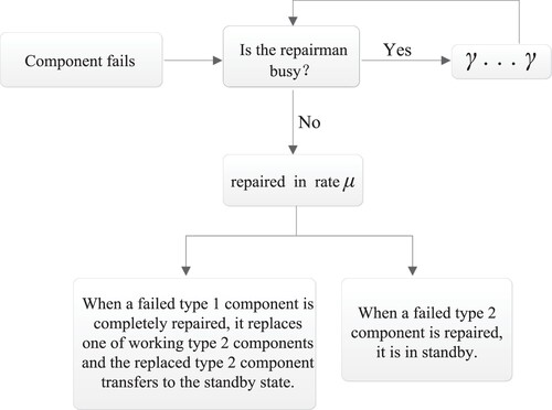
3. The failed components are repaired by a repairman who only repairs one at a time. When a component fails and the repairman is free, the failed component will be repaired immediately, otherwise if the repairman is busy with another failed component, the new failed component will enter the retrial orbit and try again after a random period of time until it is repaired. The retrial discipline for the failed components in the orbit is first in first out. Retrial times are governed by exponential distribution with parameter γ.

4. The operating time of each type 1 component and each type 2 component obeys exponential distributions with rates ${\lambda }_1$ and ${\lambda }_2$, respectively. The failure time of each warm standby type 2 component follows exponential distribution with rate $\lambda \left(\lambda <{\lambda }_1<{\lambda }_2\right)$. The time-to-repair for each failed component is exponentially distributed with rate μ, and the repaired component is as good as new.

5. The failure rate of type 1 component is lower than that of type 2, so type 1 components will be used preferentially. The priority of using discipline is the following: type 2 components are used as standby when all type 1 components in the system are normal; type 2 components start operation when the number of normal type 1 components is smaller than the minimum value for normal operation of the system; during normal operation of the system, after a failed type 1 component is repaired, it will replace one of operating type 2 components, and the replaced type 2 component will convert to standby.

6. All the random variables are independent of each other.

2.2. Model analysis

At time t, let I(t) and J(t) represent the number of failed type 1 and type 2 components in retrial orbit, respectively. K(t) describes the state of the repairman, where $\begin{array}{r}K\left(t\right)=\{\begin{array}{ll}0,& \mathrm{i}\mathrm{f}\mathrm{t}\mathrm{h}\mathrm{e}\mathrm{r}\mathrm{e}\mathrm{p}\mathrm{a}\mathrm{i}\mathrm{r}\mathrm{m}\mathrm{a}\mathrm{n}\mathrm{i}\mathrm{s}\mathrm{i}\mathrm{d}\mathrm{l}\mathrm{e}\mathrm{a}\mathrm{t}\mathrm{t}\mathrm{i}\mathrm{m}\mathrm{e}t,\\ 1_1,& \mathrm{i}\mathrm{f}\mathrm{t}\mathrm{h}\mathrm{e}\mathrm{r}\mathrm{e}\mathrm{p}\mathrm{a}\mathrm{i}\mathrm{r}\mathrm{m}\mathrm{a}\mathrm{n}\mathrm{i}\mathrm{s}\mathrm{r}\mathrm{e}\mathrm{p}\mathrm{a}\mathrm{i}\mathrm{r}\mathrm{i}\mathrm{n}\mathrm{g}\mathrm{f}\mathrm{a}\mathrm{i}\mathrm{l}\mathrm{e}\mathrm{d}\mathrm{t}\mathrm{y}\mathrm{p}\mathrm{e}1\mathrm{c}\mathrm{o}\mathrm{m}\mathrm{p}\mathrm{o}\mathrm{n}\mathrm{e}\mathrm{n}\mathrm{t}\mathrm{a}\mathrm{t}\mathrm{t}\mathrm{i}\mathrm{m}\mathrm{e}t,\\ 1_2,& \mathrm{i}\mathrm{f}\mathrm{t}\mathrm{h}\mathrm{e}\mathrm{r}\mathrm{e}\mathrm{p}\mathrm{a}\mathrm{i}\mathrm{r}\mathrm{m}\mathrm{a}\mathrm{n}\mathrm{i}\mathrm{s}\mathrm{r}\mathrm{e}\mathrm{p}\mathrm{a}\mathrm{i}\mathrm{r}\mathrm{i}\mathrm{n}\mathrm{g}\mathrm{f}\mathrm{a}\mathrm{i}\mathrm{l}\mathrm{e}\mathrm{d}\mathrm{t}\mathrm{y}\mathrm{p}\mathrm{e}2\mathrm{c}\mathrm{o}\mathrm{m}\mathrm{p}\mathrm{o}\mathrm{n}\mathrm{e}\mathrm{n}\mathrm{t}\mathrm{a}\mathrm{t}\mathrm{t}\mathrm{i}\mathrm{m}\mathrm{e}t.\end{array}\end{array}$Obviously, the state of system at time t is $\left\{K\right(t),I(t),J(t\left)\right\}$, which can be described as a Markov process $\left\{K\left(t\right),I\left(t\right),J\left(t\right),t⩾0\right\}$ with state space $\begin{array}{rl}\mathrm{\Omega }& =\left\{\left(k,i,j\right):k=0,1_1,1_2,i=0,1,\dots ,N-1,j=0,1,\dots ,N-1\right\}\cup \{\left(k,i,N\right):k=0,\\ & 1_1,i=0,1,\dots ,N-1\}\cup \left\{\left(k,N,j\right):k=0,1_2,j=0,1,\dots ,N-1\right\}.\end{array}$Based on model description and assumptions, the repair schematic diagram of failed components is shown in Figure 1. The transition rates between the system states can be described as follows.

Figure 1. The repair schematic diagram of failed components.

1. $(0,i,j)\to (1_1,i,j),i=0,1,\dots ,N-1,j=0,1,\dots ,N$: the transition occurs when a type 1 component fails and the state of the repairman changes from idle to repairing the failed type 1 component. The transition rate among this process is ${\lambda }_{(0,i,j)\to (1_1,i,j)}=(N-i){\lambda }_1$.

2. $(0,i,j)\to (1_2,i,j),i=0,1,\dots ,N,j=0,1,\dots ,N-1$: the transition occurs when a type 2 component fails and the state of the repairman changes from idle to repairing the failed type 2 component. The transition rate among this process is $\begin{array}{r}{\lambda }_{(0,i,j)\to (1_2,i,j)}=\{\begin{array}{ll}(N-j)\lambda ,& i=0,\\ i{\lambda }_2+(N-i-j)\lambda ,& N-(i+j)>0\mathrm{a}\mathrm{n}\mathrm{d}i\ne 0,\\ i{\lambda }_2,& N-(i+j)=0\mathrm{a}\mathrm{n}\mathrm{d}i\ne 0,\\ (N-j){\lambda }_2,& N-(i+j)<0\mathrm{a}\mathrm{n}\mathrm{d}i\ne 0.\end{array}\end{array}$

3. $(1_1,i,j)\to (1_1,i,j+1),i=0,1,\dots ,N-1,j=0,1,\dots ,N-1$: the transition occurs when the repairman is repairing a failed type 1 component and a type 2 component fails and enters the retrial orbit. The transition rate among this process is $\begin{array}{r}{\lambda }_{(1_1,i,j)\to (1_1,i,j+1)}=\{\begin{array}{ll}(i+1){\lambda }_2+(N-i-j-1)\lambda ,& N-(i+j)>0,\\ i{\lambda }_2,& N-(i+j)=0,\\ (N-j){\lambda }_2,& N-(i+j)<0.\end{array}\end{array}$

4. $(1_1,i,j)\to (1_1,i+1,j),i=0,1,\dots ,N-2,j=0,1,\dots ,N$: the transition occurs when the repairman is repairing a failed type 1 component and another type 1 component fails and enters the retrial orbit. The transition rate among this process is ${\lambda }_{(1_1,i,j)\to (1_1,i+1,j)}=(N-i-1){\lambda }_1$.

5. $(1_2,i,j)\to (1_2,i,j+1),i=0,1,\dots ,N,j=0,1,\dots ,N-2$: the transition occurs when the repairman is repairing a failed type 2 component and another type 2 component fails and enters the retrial orbit. The transition rate among this process is $\begin{array}{r}{\lambda }_{(1_2,i,j)\to (1_2,i,j+1)}=\{\begin{array}{ll}(N-j-1)\lambda ,& i=0,\\ i{\lambda }_2+(N-i-j-1)\lambda ,& N-(i+j+1)>0\mathrm{a}\mathrm{n}\mathrm{d}i\ne 0,\\ i{\lambda }_2,& N-(i+j+1)=0\mathrm{a}\mathrm{n}\mathrm{d}i\ne 0,\\ (N-j-1){\lambda }_2,& N-(i+j+1)<0\mathrm{a}\mathrm{n}\mathrm{d}i\ne 0.\end{array}\end{array}$

6. $(1_2,i,j)\to (1_2,i+1,j),i=0,1,\dots ,N-1,j=0,1,\dots ,N-1$: the transition occurs when the repairman is repairing a failed type 2 component and a type 1 component fails and enters the retrial orbit. The transition rate among this process is ${\lambda }_{(1_2,i,j)\to (1_2,i+1,j)}=(N-i){\lambda }_1$.

7. $(1_1,i,j)\to (0,i,j),i=0,1,\dots ,N-1,j=0,1,\dots ,N;(1_2,i,j)\to (0,i,j),i=0,1,\dots ,N,j=0,1,\dots ,N-1$: the transition occurs when the number of failed components in orbit remains unchanged and the repairman's state changes from repairing the failed type 1 or type 2 component to idle. The transition rate among this process is μ.

8. $\left(0,i,j\right)\to \left(1_1,i-1,j\right),i=1,2,\dots ,N-1,j=0,1,\dots ,N;\left(0,N,j\right)\to \left(1_1,N-1,j\right),j=0,1,\dots ,N-1$: the transition occurs when a failed type 1 in the orbit retries successfully and the repairman repairs the failed type 1 component. The transition rate among this process is γ.

9. $\left(0,i,j\right)\to \left(1_2,i,j-1\right),i=0,1,\dots ,N-1,j=1,2,\dots ,N;\left(0,N,j\right)\to \left(1_2,N,j-1\right),j=1,2,\dots ,N-1$: the transition occurs when a failed type 2 in the orbit retries successfully and the repairman repairs the failed type 2 component. The transition rate among this process is γ.

3. Performance index analysis

3.1. System transition rate matrix

Based on the state transition of system and division of idle and busy states of the repairman, the system transition rate matrix $\mathbf{\text{Q}}$ of order $3N^2+4N$ can be regarded as a block matrix, which is described as follows: $\begin{array}{r}\mathbf{\text{Q}}=\left(\begin{array}{cc}{\mathbf{\text{Q}}}_1& {\mathbf{\text{Q}}}_2\\ {\mathbf{\text{Q}}}_3& {\mathbf{\text{Q}}}_4\end{array}\right).\end{array}$According to the division of the number of failed type 1 and type 2 components in the retrial orbit, the sub-blocks ${\mathbf{\text{Q}}}_1$, ${\mathbf{\text{Q}}}_2$, ${\mathbf{\text{Q}}}_3$ and ${\mathbf{\text{Q}}}_4$ of the matrix $\mathbf{\text{Q}}$ can be expressed as follows: $\begin{array}{rlr}& \left(1\right){\mathbf{\text{Q}}}_1={\left(\begin{array}{ccccc}{\mathbf{\text{Q}}}_0^{\mathrm{\prime }}& & & & \\ & {\mathbf{\text{Q}}}_1^{\mathrm{\prime }}& & & \\ & & \ddots & & \\ & & & {\mathbf{\text{Q}}}_{N-1}^{\mathrm{\prime }}& \\ & & & & {\mathbf{\text{Q}}}_N^{\mathrm{\prime }}\end{array}\right)}_{(N^2+2N)\times (N^2+2N)},& \end{array}$where

${\mathbf{\text{Q}}}_0^{\prime }=\mathrm{d}\mathrm{i}\mathrm{a}\mathrm{g}(-(N{\lambda }_1+N\lambda ),-(\gamma +N{\lambda }_1+(N-1)\lambda ),\dots ,-(\gamma +N{\lambda }_1+\lambda ),-(\gamma +N{\lambda }_1\left)\right),$ with the order of ${\mathbf{\text{Q}}}_0^{\prime }$ being $N+1,$ $\begin{array}{rl}{\mathbf{\text{Q}}}_i^{\prime }& =\mathrm{d}\mathrm{i}\mathrm{a}\mathrm{g}(-(\gamma +(N-i){\lambda }_1+i{\lambda }_2+(N-i)\lambda ),-(2\gamma +(N-i){\lambda }_1+i{\lambda }_2+(N-i-1)\lambda ),\dots ,\\ & -(2\gamma +(N-i){\lambda }_1+i{\lambda }_2+\lambda ),-(2\gamma +(N-i){\lambda }_1+i{\lambda }_2),-(2\gamma +(N-i){\lambda }_1\\ & +(i-1){\lambda }_2),-(2\gamma +(N-i){\lambda }_1+(i-2){\lambda }_2),\dots ,-(2\gamma +(N-i){\lambda }_1+{\lambda }_2),-(2\gamma \\ & +(N-i){\lambda }_1\left)\right),i=1,2,\dots ,N-1(N⩾2),\end{array}$with the order of ${\mathbf{\text{Q}}}_i^{\prime }$ being $N+1,$

${\mathbf{\text{Q}}}_N^{\prime }=\mathrm{d}\mathrm{i}\mathrm{a}\mathrm{g}(-(\gamma +N{\lambda }_2),-(2\gamma +(N-1){\lambda }_2),\dots ,-(2\gamma +{\lambda }_2\left)\right),$ with the order of ${\mathbf{\text{Q}}}_N^{\prime }$ being N. $\begin{array}{rl}& \left(2\right){\mathbf{\text{Q}}}_2={\left({\mathbf{\text{Q}}}_{21}{\mathbf{\text{Q}}}_{22}\right)}_{(N^2+2N)\times (2N^2+2N)},\end{array}$and the sub-blocks ${\mathbf{\text{Q}}}_{21}$ and ${\mathbf{\text{Q}}}_{22}$ can be divided according to the number of failed components of type 1 and type 2 in the retrial orbit, as below: $\begin{array}{rl}{\mathbf{\text{Q}}}_{21}& ={\left(\begin{array}{ccccc}{\mathbf{\text{A}}}_0& & & & \\ {\mathbf{\text{B}}}_1& {\mathbf{\text{A}}}_1& & & \\ & {\mathbf{\text{B}}}_2& {\mathbf{\text{A}}}_2& & \\ & & \ddots & \ddots & \\ & & & {\mathbf{\text{B}}}_{N-1}& {\mathbf{\text{A}}}_{N-1}\\ & & & & {\mathbf{\text{B}}}_N\end{array}\right)}_{(N^2+2N)\times (N^2+N)},\\ {\mathbf{\text{Q}}}_{22}& ={\left(\begin{array}{ccccc}{\mathbf{\text{C}}}_0& & & & \\ & {\mathbf{\text{C}}}_1& & & \\ & & \ddots & & \\ & & & {\mathbf{\text{C}}}_{N-1}& \\ & & & & {\mathbf{\text{C}}}_N\end{array}\right)}_{(N^2+2N)\times (N^2+N)},\end{array}$where

${\mathbf{\text{A}}}_i=\mathrm{d}\mathrm{i}\mathrm{a}\mathrm{g}\left(\right(N-i){\lambda }_1,\dots ,(N-i\left){\lambda }_1\right),i=0,1,\dots ,N-1,$ with the order of ${\mathbf{\text{A}}}_i$ being $N+1,$

${\mathbf{\text{B}}}_i=\mathrm{d}\mathrm{i}\mathrm{a}\mathrm{g}(\gamma ,\dots ,\gamma ),i=1,2,\dots ,N-1(N⩾2),$ with the order of ${\mathbf{\text{B}}}_i$ being $N+1,$

${\mathbf{\text{B}}}_N=(\mathbf{\text{B}}\mathbf{\text{0}}{)}_{N\times (N+1)},$

$\mathbf{\text{B}}=\mathrm{d}\mathrm{i}\mathrm{a}\mathrm{g}(\gamma ,\dots ,\gamma ),$ with the order of $\mathbf{\text{B}}$ being N, and $\mathbf{\text{0}}=(0,\dots ,0{)}_{1\times N}^{\mathrm{\top }}$, $\begin{array}{r}{\mathbf{\text{C}}}_i={\left(\begin{array}{cccccccc}i{\lambda }_2+(N-i)\lambda & & & & & & & \\ \gamma & i{\lambda }_2+(N-i-1)\lambda & & & & & & \\ & \gamma & \ddots & & & & & \\ & & \ddots & i{\lambda }_2+\lambda & & & & \\ & & & \gamma & i{\lambda }_2& & & \\ & & & & \gamma & (i-1){\lambda }_2& & \\ & & & & & \ddots & \ddots & \\ & & & & & & \gamma & {\lambda }_2\\ & & & & & & & \gamma \end{array}\right)}_{(N+1)\times N},\end{array}$$i=0,1,\dots ,N-1,$ and $\begin{array}{rl}{\mathbf{\text{C}}}_N& ={\left(\begin{array}{cccc}i{\lambda }_2& & & \\ \gamma & (i-1){\lambda }_2& & \\ & \gamma & \ddots & \\ & & \ddots & 2{\lambda }_2\\ & & & \gamma \end{array}\begin{array}{c}\\ \\ \\ \\ {\lambda }_2\end{array}\right)}_{N\times N}.\\ \left(3\right){\mathbf{\text{Q}}}_3& ={\left(\begin{array}{c}{\mathbf{\text{Q}}}_{31}\\ {\mathbf{\text{Q}}}_{32}\end{array}\right)}_{(2N^2+2N)\times (N^2+2N)},\end{array}$and the sub-blocks ${\mathbf{\text{Q}}}_{31}$ and ${\mathbf{\text{Q}}}_{32}$ can be divided according to the number of failed components of type 1 and type 2 in the retrial orbit, as below: $\begin{array}{rl}{\mathbf{\text{Q}}}_{31}& ={\left({\mathbf{\text{D}}}_1{\mathbf{\text{D}}}_2\right)}_{(N^2+N)\times (N^2+2N)},\\ {\mathbf{\text{Q}}}_{32}& ={\left(\begin{array}{ccccc}{\mathbf{\text{L}}}_0& & & & \\ & {\mathbf{\text{L}}}_1& & & \\ & & \ddots & & \\ & & & {\mathbf{\text{L}}}_{N-1}& \\ & & & & {\mathbf{\text{L}}}_N\end{array}\right)}_{(N^2+N)\times (N^2+2N)},\end{array}$where

${\mathbf{\text{D}}}_1=\mathrm{d}\mathrm{i}\mathrm{a}\mathrm{g}(\mu ,\dots ,\mu ),$ with the order of ${\mathbf{\text{D}}}_1$ being $N^2+N,$ ${\mathbf{\text{D}}}_2={\mathbf{\text{0}}}_{(N^2+N)\times N},$

${\mathbf{\text{L}}}_i=(\mathbf{\text{L}}\mathbf{\text{0}}{)}_{N\times (N+1)},i=0,1,\dots ,N-1,\mathbf{\text{L}}=\mathrm{d}\mathrm{i}\mathrm{a}\mathrm{g}(\mu ,\dots ,\mu ),$ with the order of $\mathbf{\text{L}}$ being $N,\mathbf{\text{0}}=(0,\dots ,0{)}_{1\times N}^{\mathrm{\top }},$ and ${\mathbf{\text{L}}}_N=\mathbf{\text{L}}$. $\begin{array}{r}\left(4\right){\mathbf{\text{Q}}}_4={\left(\begin{array}{cc}{\mathbf{\text{Q}}}_{41}& \\ & {\mathbf{\text{Q}}}_{42}\end{array}\right)}_{(2N^2+2N)\times (2N^2+2N)},\end{array}$and the sub-blocks ${\mathbf{\text{Q}}}_{41}$ and ${\mathbf{\text{Q}}}_{42}$ can be divided according to the number of failed components of type 1 and type 2 in the retrial orbit, as below: $\begin{array}{rl}{\mathbf{\text{Q}}}_{41}& ={\left(\begin{array}{ccccc}{\mathbf{\text{H}}}_0& {\mathbf{\text{A}}}_0^{\mathrm{\prime }}& & & \\ & {\mathbf{\text{H}}}_1& {\mathbf{\text{A}}}_1^{\mathrm{\prime }}& & \\ & & \ddots & \ddots & \\ & & & {\mathbf{\text{H}}}_{N-2}& {\mathbf{\text{A}}}_{N-2}^{\mathrm{\prime }}\\ & & & & {\mathbf{\text{H}}}_{N-1}\end{array}\right)}_{(N^2+N)\times (N^2+N)},\\ {\mathbf{\text{Q}}}_{42}& ={\left(\begin{array}{ccccc}{\mathbf{\text{T}}}_0& {\mathbf{\text{V}}}_0& & & \\ & {\mathbf{\text{T}}}_1& {\mathbf{\text{V}}}_1& & \\ & & \ddots & \ddots & \\ & & & {\mathbf{\text{T}}}_{N-1}& {\mathbf{\text{V}}}_{N-1}\\ & & & & {\mathbf{\text{T}}}_N\end{array}\right)}_{(N^2+N)\times (N^2+N)},\end{array}$where

${\mathbf{\text{A}}}_i^{\prime }=\mathrm{d}\mathrm{i}\mathrm{a}\mathrm{g}\left(\right(N-i-1){\lambda }_1,\dots ,(N-i-1\left){\lambda }_1\right),$ $i=0,1,\dots ,N-2,$ with the order of ${\mathbf{\text{A}}}_i^{\prime }$ being $N+1.$ $\begin{array}{r}{\mathbf{\text{H}}}_i={\left(\begin{array}{ccccccccc}{\psi }_1& {\varphi }_1& & & & & & & \\ & {\psi }_2& {\varphi }_2& & & & & & \\ & & \ddots & \ddots & & & & & \\ & & & {\psi }_{l-1}& {\varphi }_{l-1}& & & & \\ & & & & {\psi }_l& {\varphi }_l& & & \\ & & & & & {\psi }_{l+1}& {\varphi }_{l+1}& & \\ & & & & & & \ddots & \ddots & \\ & & & & & & & {\psi }_N& {\varphi }_N\\ & & & & & & & & {\psi }_{N+1}\end{array}\right)}_{(N+1)\times (N+1)},\end{array}$$i=0,1,\dots ,N-1,$ where $\begin{array}{rl}{\psi }_1& =-(\mu +(N-i-1){\lambda }_1+(i+1){\lambda }_2+(N-i-1\left)\lambda \right),{\varphi }_1=(i+1){\lambda }_2+(N-i-1)\lambda ,\\ {\psi }_2& =-(\mu +(N-i-1){\lambda }_1+(i+1){\lambda }_2+(N-i-2\left)\lambda \right),{\varphi }_2=(i+1){\lambda }_2+(N-i-2)\lambda ,\\ {\psi }_{l-1}& =-(\mu +(N-i-1){\lambda }_1+(i+1){\lambda }_2+\lambda ),{\varphi }_{l-1}=(i+1){\lambda }_2+\lambda ,\\ {\psi }_l& =-(\mu +(N-i-1){\lambda }_1+(i+1\left){\lambda }_2\right),{\varphi }_l=(i+1){\lambda }_2,\\ {\psi }_{l+1}& =-(\mu +(N-i-1){\lambda }_1+i{\lambda }_2),{\varphi }_{l+1}=i{\lambda }_2,\\ {\psi }_N& =-(\mu +(N-i-1){\lambda }_1+{\lambda }_2),{\varphi }_N={\lambda }_2,\\ {\psi }_{N+1}& =-(\mu +(N-i-1\left){\lambda }_1\right).\end{array}$${\mathbf{\text{V}}}_i=\mathrm{d}\mathrm{i}\mathrm{a}\mathrm{g}\left(\right(N-i){\lambda }_1,\dots ,(N-i\left){\lambda }_1\right),$ $i=0,1,\dots ,N-1,$ with the order of ${\mathbf{\text{V}}}_i$ being N. $\begin{array}{r}{\mathbf{\text{T}}}_i={\left(\begin{array}{ccccccccc}{\text{β}}_1& {\phi }_1& & & & & & & \\ & \text{β}{}_2& {\phi }_2& & & & & & \\ & & \ddots & \ddots & & & & & \\ & & & \text{β}{}_{l-1}& {\phi }_{l-1}& & & & \\ & & & & {\text{β}}_l& {\phi }_l& & & \\ & & & & & {\text{β}}_{l+1}& {\phi }_{l+1}& & \\ & & & & & & \ddots & \ddots & \\ & & & & & & & {\text{β}}_{N-1}& {\phi }_{N-1}\\ & & & & & & & & {\text{β}}_N\end{array}\right)}_{N\times N},\end{array}$$i=0,1,\dots ,N-1,$ where $\begin{array}{rl}{\text{β}}_1& =-(\mu +(N-i){\lambda }_1+i{\lambda }_2+(N-i-1\left)\lambda \right),{\phi }_1=i{\lambda }_2+(N-i-1)\lambda ,\\ {\text{β}}_2& =-(\mu +(N-i){\lambda }_1+i{\lambda }_2+(N-i-2\left)\lambda \right),{\phi }_2=i{\lambda }_2+(N-i-2)\lambda ,\\ {\text{β}}_{l-1}& =-(\mu +(N-i){\lambda }_1+i{\lambda }_2+\lambda ),{\phi }_{l-1}=i{\lambda }_2+\lambda ,\\ {\text{β}}_l& =-(\mu +(N-i){\lambda }_1+i{\lambda }_2),{\phi }_l=i{\lambda }_2,\\ {\text{β}}_{l+1}& =-(\mu +(N-i){\lambda }_1+(i-1\left){\lambda }_2\right),{\phi }_{l+1}=(i-1){\lambda }_2,\\ {\text{β}}_{N-1}& =-(\mu +(N-i){\lambda }_1+{\lambda }_2),{\phi }_{N-1}={\lambda }_2,\\ {\text{β}}_N& =-(\mu +(N-i\left){\lambda }_1\right).\\ {\mathbf{\text{T}}}_N& ={\left(\begin{array}{ccccc}-(\mu +(i-1\left){\lambda }_2\right)& (i-1){\lambda }_2& & & \\ & -(\mu +(i-2\left){\lambda }_2\right)& (i-2){\lambda }_2& & \\ & & \ddots & \ddots & \\ & & & -(\mu +{\lambda }_2)& {\lambda }_2\\ & & & & -\mu \end{array}\right)}_{N\times N}.\end{array}$

3.2. Steady state performance indices

Under steady-state conditions, the state probability of the system can be expressed as $P_{k,ij}=\underset{t\to \mathrm{\infty }}{lim}{P}_{k,ij}\left(t\right),k,i,j\in \mathrm{\Omega }.$Let $\begin{array}{rl}{\mathbf{\text{P}}}_{0,i}& =(P_{0,i0},P_{0,i1},\dots ,P_{0,iN}),i=0,1,\dots ,N-1,\\ {\mathbf{\text{P}}}_{0,N}& =(P_{0,N0},P_{0,N1},\dots ,P_{0,N(N-1)}),\\ {\mathbf{\text{P}}}_{1_1,i}& =(P_{1_1,i0},P_{1_1,i1},\dots ,P_{1_1,iN}),i=0,1,\dots ,N-1,\\ {\mathbf{\text{P}}}_{1_2,i}& =(P_{1_2,i0},P_{1_2,i1},\dots ,P_{1_2,i(N-1)}),i=0,1,\dots ,N.\end{array}$The matrix form of system state probability equations under steady-state conditions can be written as follows: (1) $\mathbf{\text{P}}\mathbf{\text{Q}}=\mathbf{\text{0}},$(1) where $\mathbf{\text{P}}=({\mathbf{\text{P}}}_{0,0},{\mathbf{\text{P}}}_{0,1},\dots ,{\mathbf{\text{P}}}_{0,N-1},{\mathbf{\text{P}}}_{0,N},{\mathbf{\text{P}}}_{1_1,0},{\mathbf{\text{P}}}_{1_1,1},\dots ,{\mathbf{\text{P}}}_{1_1,N-1},{\mathbf{\text{P}}}_{1_2,0},{\mathbf{\text{P}}}_{1_2,1},\dots ,{\mathbf{\text{P}}}_{1_2,N})$, and $\mathbf{\text{0}}$ is a row vector of order $3N^2+4N$.

The normalization condition is (2) $\sum _{i=0}^{N-1}\sum _{j=0}^N{P}_{0,ij}+\sum _{j=0}^{N-1}{P}_{0,Nj}+\sum _{i=0}^{N-1}\sum _{j=0}^N{P}_{1_1,ij}+\sum _{i=0}^N\sum _{j=0}^{N-1}{P}_{1_2,ij}=1.$(2) Based on Equations (1(1) $\mathbf{\text{P}}\mathbf{\text{Q}}=\mathbf{\text{0}},$(1) ) and (2(2) $\sum _{i=0}^{N-1}\sum _{j=0}^N{P}_{0,ij}+\sum _{j=0}^{N-1}{P}_{0,Nj}+\sum _{i=0}^{N-1}\sum _{j=0}^N{P}_{1_1,ij}+\sum _{i=0}^N\sum _{j=0}^{N-1}{P}_{1_2,ij}=1.$(2) ), the steady-state probabilities of the system can be calculated by using Crammer's rule.

• The steady-state availability of the system can be given by (3) $A\left(\mathrm{\infty }\right)=1-\sum _{i+j>N}{P}_{0,ij}-\sum _{i+j>N-1}{P}_{1_1,ij}-\sum _{i+j>N-1}{P}_{1_2,ij}.$(3)

• Mean number of failed type 1 components in the orbit is (4) $\mathrm{E}\left(N_1\right)=\sum _{i=0}^{N-1}i\times \left(\sum _{j=0}^N{P}_{0,ij}+\sum _{j=0}^N{P}_{1_1,ij}+\sum _{j=0}^{N-1}{P}_{1_2,ij}\right)+N\times \sum _{j=0}^{N-1}\left(P_{0,Nj}+P_{1_2,Nj}\right).$(4)

• Mean number of failed type 2 components in the orbit is (5) $\mathrm{E}\left(N_2\right)=\sum _{j=0}^{N-1}j\times \left(\sum _{i=0}^N{P}_{0,ij}+\sum _{i=0}^{N-1}{P}_{1_1,ij}+\sum _{i=0}^N{P}_{1_2,ij}\right)+N\times \sum _{i=0}^{N-1}\left(P_{0,iN}+P_{1_1,iN}\right).$(5)

• The probability that the repairman is in idle state is (6) $P_I=\sum _{i=0}^{N-1}\sum _{j=0}^N{P}_{0,ij}+\sum _{j=0}^{N-1}{P}_{0,Nj}.$(6)

• The probability that the repairman is repairing a failed type 1 component is (7) $P_{b_1}=\sum _{i=0}^{N-1}\sum _{j=0}^N{P}_{1_1,ij}.$(7)

• The probability that the repairman is repairing a failed type 2 component is (8) $P_{b_2}=\sum _{i=0}^N\sum _{j=0}^{N-1}{P}_{1_2,ij}.$(8)

3.3. Bayesian parameter estimation

In this section, we estimate the system parameters ${\lambda }_1,{\lambda }_2,\lambda ,\mu ,\gamma$ by Bayesian approach.

Suppose that the population $S_1=\left(S_{11},S_{12},\dots ,S_{1g_1}\right)$ is independent and identically distributed exponential random variables with parameter${\lambda }_1$. The likelihood function of ${\lambda }_1$ for sample $S_1$ is given by $L\left({\lambda }_1\mid S_1\right)={\lambda }_1^{g_1}{\mathrm{e}}^{-{\lambda }_1{X}_1}$, where $X_1=S_{11}+S_{12}+\cdots +S_{1g_1}$. Then, suppose that the prior distribution of failure rate ${\lambda }_1$ is Gamma distribution with parameters $m_1$ and $n_1$, denoted by ${\lambda }_1\sim G\left(m_1,n_1\right)$, whose density function is given by $f\left({\lambda }_1\right)=\frac{n_1^{m_1}}{\mathrm{\Gamma }\left(m_1\right)}{\lambda }_1^{m_1-1}{\mathrm{e}}^{-{\lambda }_1{n}_1}$. Mathematical expectation $\mathrm{E}\left({\lambda }_1\right)=\frac{m_1}{n_1}$, and variance $\mathrm{V}\mathrm{a}\mathrm{r}\left({\lambda }_1\right)=\frac{m_1}{{n_1}^2}$. Using the Bayesian formula, we can obtain the posterior probability density function of parameter ${\lambda }_1$ for given sample $S_1$, which is $\pi \left({\lambda }_1\mid S_1\right)=\frac{{\left(n_1+S_1\right)}^{g_1+m_1}}{\mathrm{\Gamma }\left(g_1+m_1\right)}{\lambda }_1^{g_1+m_1-1}{\mathrm{e}}^{-{\lambda }_1\left(n_1+S_1\right)}$, denoted by ${\lambda }_1\sim G\left(g_1+m_1,n_1+S_1\right)$. Under the square loss function, the Bayesian estimate of parameter ${\lambda }_1$ is the posterior mean of ${\lambda }_1$, denoted as ${\hat{\lambda }}_1=\frac{g_1+m_1}{n_1+S_1}$.

Similarly, the Bayes estimators of ${\lambda }_2,\lambda ,\mu$ and γ can be obtained. Then, we can obtain the joint posterior distribution of ${\lambda }_1,{\lambda }_2,\lambda ,\mu$ and γ. By Monte Carlo simulation methods, the parameters ${\lambda }_1,{\lambda }_2,\lambda ,\mu$ and γ can be estimated. Finally, we substitute ${\lambda }_1,{\lambda }_2,\lambda ,\mu$ and γ in Equations (3(3) $A\left(\mathrm{\infty }\right)=1-\sum _{i+j>N}{P}_{0,ij}-\sum _{i+j>N-1}{P}_{1_1,ij}-\sum _{i+j>N-1}{P}_{1_2,ij}.$(3) )–(8(8) $P_{b_2}=\sum _{i=0}^N\sum _{j=0}^{N-1}{P}_{1_2,ij}.$(8) ) to obtain the corresponding performance indices.

3.4. Cost-benefit ratio

Cost is an important index that needs to be evaluated in practical engineering. It has attracted attention of many scholars (see, for example, Kuo et al., 2014; Zhao & Guo et al., 2018; Zhao & Wang et al., 2018; Meena et al., 2019; Yen & Wang, 2020; Kumar & Jain, 2020; Wu et al., 2021; Gao & Wang, 2021). There are many factors that affect the total system cost, such as component failure rate, retrial rate, repair rate, the number of standby components and so on. Meena et al. (2019) and Kumar and Jain (2020) both considered the cost of repairman and failed components. The former constructed a function of the total cost per unit time, in which the repair rate and vacation rate are the decision variables, while the latter constructed a function of the expected total cost at time t regarding the repair rate. However, the benefit of the system should also be considered while maintaining the smaller total cost conditions, so cost-benefit analysis is an important part of the system design. Based on the cost models in Meena et al. (2019) and Kumar and Jain (2020), we develop a cost-benefit ratio optimization model. The cost-benefit ratio is the ratio of expected total cost and availability per unit time under steady-state condition. In this work, it mainly studies the influence of decision variable μ on the cost-benefit ratio of the system and finds an appropriate one that minimizes the cost-benefit ratio.

The per-unit cost elements on constructing the cost model are defined as follows:

• $C_{h_1}$: cost incurred on failed type 1 components in orbit,

• $C_{h_2}$: cost incurred on failed type 2 components in orbit,

• $C_n$: cost for repairman in idle,

• $C_{b_1}$: cost incurred on repairman who is busy repairing a failed type 1 component,

• $C_{b_2}$: cost incurred on repairman who is busy repairing a failed type 2 component,

• $C_{r_1}$: cost incurred on the repair job for failed type 1 components with rate μ,

• $C_{r_2}$: cost incurred on the repair job for failed type 2 components with rate μ.

Using the above cost elements and the corresponding system performance indices, the expected total cost function is formulated as follows (9) $\mathrm{T}\mathrm{C}\left(\mu \right)=C_{h_1}\mathrm{E}\left(N_1\right)+C_{h_2}\mathrm{E}\left(N_2\right)+C_n{P}_I+C_{b_1}{P}_{b_1}+C_{b_2}{P}_{b_2}+C_{r_1}\mu +C_{r_2}\mu .$(9) Taking $\mathrm{T}\mathrm{C}\left(\mu \right)$ as the numerator and $A\left(\mathrm{\infty }\right)$ as the denominator of the cost-benefit ratio, an optimization model of the cost-benefit ratio is given by (10) $\mathrm{m}\mathrm{i}\mathrm{n}\frac{C_{h_1}\mathrm{E}\left(N_1\right)+C_{h_2}\mathrm{E}\left(N_1\right)+C_n{P}_I+C_{b_1}{P}_{b_1}+C_{b_2}{P}_{b_2}+C_{r_1}\mu +C_{r_2}\mu }{{\displaystyle 1-\sum _{i+j>N}{P}_{0,ij}-\sum _{i+j>N-1}{P}_{1_1,ij}-\sum _{i+j>N-1}{P}_{1_2,ij}}},$(10) subject to $\mu >0$.

4. Numerical results

In some real manufacturing engineering systems, the failure of machine or product equipment can reduce production output, which can be ameliorated by the support of repair facility and standby machines. An application of our model can be realized in a retrial machine repair system with warm standby units, which consists of two type 1 units, two type 2 units and a single repair server. The system works normally only if there are two or more units in operation. We take ${\lambda }_1=0.10$, ${\lambda }_2=0.16$, $\lambda =0.008$, $\mu =1.0$, and $\gamma =1.2$ as the basic parameter values (They can be estimated by the Bayesian approach in Section 3.3). According to the theoretical results provided in Section 3, the system steady-state availability and cost-benefit ratio are analyzed numerically. Based on default values, we obtain $A\left(\mathrm{\infty }\right)$= 0.982.

4.1. Numerical analysis for steady-state availability

By choosing ${\lambda }_1$ or ${\lambda }_2$ as one of each pair and one of the rest system parameters as another, we analyze the effect of system parameters on $A\left(\mathrm{\infty }\right)$. The results are shown in Figures 2–5.

Figure 2. Effect of ${\lambda }_1$ and ${\lambda }_2$ on $A\left(\mathrm{\infty }\right)$.

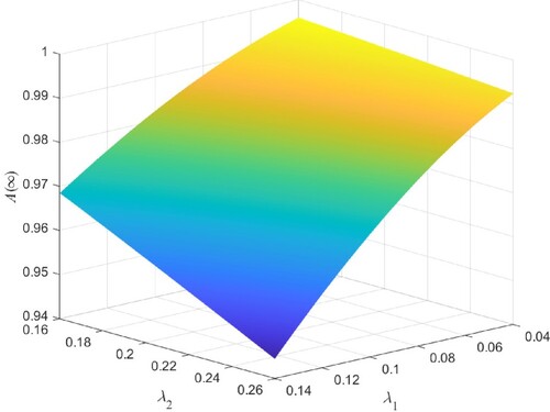
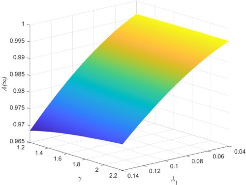
Figure 2 shows the three-dimensional graph of $A\left(\mathrm{\infty }\right)$ by varying ${\lambda }_1$ from 0.04 to 0.14 and ${\lambda }_2$ from 0.16 to 0.26. We observe from Figure 2 that $A\left(\mathrm{\infty }\right)$ decreases with the increase of ${\lambda }_1$ or ${\lambda }_2$, and the effect of ${\lambda }_2$ on $A\left(\mathrm{\infty }\right)$ is smaller than that of ${\lambda }_1$. This is because with the failure rate of type 1 or type 2 unit increases, the system will more easily break down. In Figure 3, $A\left(\mathrm{\infty }\right)$ decreases as the value of λ increases from 0.006 to 0.016. On the contrary, Figures 4 and 5 show the increasing trend of $A\left(\mathrm{\infty }\right)$ as μ increases from 1.0 to 2.0 and γ increases from 1.2 to 2.2, respectively. The reason is that higher repair rate and retrial rate can make failed units return to normal state faster. Therefore, increasing them can improve the steady-state availability of the system. Besides, we also observe from Figures 2–5 that ${\lambda }_1$ and μ affect $A\left(\mathrm{\infty }\right)$ significantly, and ${\lambda }_2$ affects $A\left(\mathrm{\infty }\right)$ moderately, while λ and γ affect $A\left(\mathrm{\infty }\right)$ slightly.

Figure 3. Effect of ${\lambda }_1$ and λ on $A\left(\mathrm{\infty }\right)$.

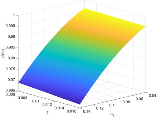
Figure 4. Effect of ${\lambda }_1$ and μ on $A\left(\mathrm{\infty }\right)$.

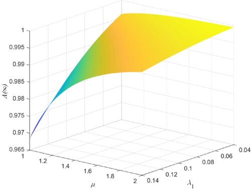
Figure 5. Effect of ${\lambda }_1$ and γ on $A\left(\mathrm{\infty }\right)$.

4.2. Numerical analysis for cost-benefit ratio

The effect of repair rate on system cost-benefit ratio is investigated for the retrial machine repair problem with two types of units. For the calculation of performance indices, the default parameters are assumed as $C_{h_1}=\mathrm{\$}70$, $C_{h_2}=\mathrm{\$}80$, $C_n=\mathrm{\$}30$, $C_{b_1}=\mathrm{\$}50$, $C_{b_2}=\mathrm{\$}55$, $C_{r_1}=\mathrm{\$}40$, $C_{r_2}=\mathrm{\$}45$, and the system cost-benefit ratio with respect to repair rate μ can be numerically calculated. Numerical results in Figure 6 indicate the effect of repair rate μ on some performance indices of the system, where $\mathrm{E}\left(N_1\right)$, $\mathrm{E}\left(N_2\right)$, $P_{b_1}$ and $P_{b_2}$ decrease as the increase of μ. 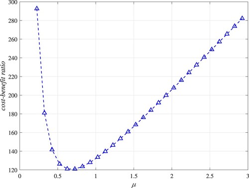On the contrary, $P_I$ shows an increasing trend as μ grows up. As shown in Figure 7, the cost-benefit ratio first decreases and then increases with the increase of μ, and there is an optimal value ${\mu }^{\ast }$ to minimize the cost-benefit ratio. Through MATLAB software, we can obtain the optimal repair rate ${\mu }^{\ast }$(0.676) and the minimum value of cost-benefit ratio (120.524). Furthermore, we find that the system availability is 0.951 when the cost-benefit ratio is minimized.

Figure 6. The effect of μ on $\mathrm{E}\left(N_1\right)$, $\mathrm{E}\left(N_2\right)$, $P_{b_1}$ and $P_{b_2}$.

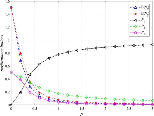
Figure 7. The effect of μ on cost-benefit ratio.

5. Conclusions

This paper proposes a warm standby repairable retrial system model with non-identical components and operating priority. The system steady state performance indices are analyzed by using Markov process theory and matrix analytical method. By Bayesian approach, the basic estimation idea of estimating system parameters with gamma prior distribution is provided. A minimum optimization model of system cost-benefit ratio with repair rate as decision variable is constructed. Numerical examples demonstrate how the system parameters affect the system steady-state availability, and the effect of repair rate on the cost-benefit ratio of the system. The important numerical results are summarized as follows. (i) The change of type 1 component failure rate on system steady-state availability is more affected than that of type 2 component. (ii) Through optimization analysis, the optimal repair rate is obtained, which makes the cost-benefit ratio of the system minimum. The numerical results provide a reference for decision-maker of the system in selecting the parameter values, so as to better design the system.

However, the limitations of this system model are the assumptions on exponential distribution, and the same number of type 1 and type 2 components. In the future, a potential work is to consider that the failure time and repair time are assumed to follow phase-type distribution. Another potential work is to extend the number of type 1 and type 2 components to make it more general.

Disclosure statement

No potential conflict of interest was reported by the authors.

Additional information

Funding

This work was supported by the National Natural Science Foundation of China [Grant Number 72071175, 72001070].

References

- Amari, S. V., Pham, H., & Misra, R. B. (2012). Reliability characteristics of k-out-of-n warm standby systems. IEEE Transactions on Reliability, 61(4), 1007–1018. https://doi.org/10.1109/tr.2012.2220891
- Chen, W. L., & Wang, K. H. (2018). Reliability analysis of a retrial machine repair problem with warm standbys and a single server with N-policy. Reliability Engineering & System Safety, 180, 476–486. https://doi.org/10.1016/j.ress.2018.08.011
- El-Damcese, M. A. (2009). Analysis of warm standby systems subject to common-cause failures with time varying failure and repair rates. Applied Mathematical Sciences, 3(18), 853–860. http://www.m-hikari.com/ams/ams-password-2009/ams-password17-20-2009/eldamceseAMS17-20-2009.pdf
- Gao, S (2021). Availability and reliability analysis of a retrial system with warm standbys and second optional repair service. Communications in Statistics-Theory and Methods1–19. https://doi.org/10.1080/03610926.2021.1922702
- Gao, S., & Wang, J (2021). Reliability and availability analysis of a retrial system with mixed standbys and an unreliable repair facility. Reliability Engineering & System Safety, 205, 107240. https://doi.org/10.1016/j.ress.2020.107240
- Hsu, Y. L., Lee, S. L., & Ke, J. C (2009). A repairable system with imperfect coverage and reboot: Bayesian and asymptotic estimation. Mathematics and Computers in Simulation, 79(7), 2227–2239. https://doi.org/10.1016/j.matcom.2008.12.018
- Janssens, G. K (1997). The quasi-random input queueing system with repeated attempts as a model for a collision-avoidance star local area network. IEEE Transactions on Communications, 45(3), 360–364. https://doi.org/10.1109/26.558699
- Ke, J. C., Yang, D. Y., S. H. Sheu, & Kuo, C. C (2013). Availability of a repairable retrial system with warm standby components. International Journal of Computer Mathematics, 90(11), 2279–2297. https://doi.org/10.1080/00207160.2013.783695
- Krishnamoorthy, A., & Ushakumari, P. V (1999). Reliability of a k-out-of-n system with repair and retrial of failed units. Top, 7(2), 293–304. https://doi.org/10.1007/BF02564728
- Kumar, P., & Jain, M (2020). Reliability analysis of a multi-component machining system with service interruption, imperfect coverage, and reboot. Reliability Engineering & System Safety, 202, 106991. https://doi.org/10.1016/j.ress.2020.106991
- Kuo, C. C., Sheu, S. H., Ke, J. C., & Zhang, Z. G (2014). Reliability-based measures for a retrial system with mixed standby components. Applied Mathematical Modelling, 38(19-20), 4640–4651. https://doi.org/10.1016/j.apm.2014.03.005
- Levitin, G., Finkelstein, M., & Dai, Y (2021). Optimal shock-driven switching strategies with elements reuse in heterogeneous warm-standby systems. Reliability Engineering & System Safety, 210, 107517. https://doi.org/10.1016/j.ress.2021.107517
- Meena, R. K., Jain, M., Sanga, S. S., & Assad, A (2019). Fuzzy modeling and harmony search optimization for machining system with general repair, standby support and vacation. Applied Mathematics and Computation, 361, 858–873. https://doi.org/10.1016/j.amc.2019.05.053
- Pustova, S. V (2010). Investigation of call centers as retrial queuing systems. Cybernetics and Systems Analysis, 46(3), 494–499. https://doi.org/10.1007/s10559-010-9224-z
- She, J., & Pecht, M. G (1992). Reliability of a k-out-of-n warm-standby system. IEEE Transactions on Reliability, 41(1), 72–75. https://doi.org/10.1109/24.126674
- Singh, J (1989). A warm standby redundant system with common cause failures. Reliability Engineering & System Safety, 26(2), 135–141. https://doi.org/10.1016/0951-8320(89)90070-7
- Srinivasan, S. K., & Subramanian, R (2006). Reliability analysis of a three unit warm standby redundant system with repair. Annals of Operations Research, 143(1), 227–235. https://doi.org/10.1007/s10479-006-7384-z
- Tran-Gia, P., & Mandjes, M (1997). Modeling of customer retrial phenomenon in cellular mobile networks. IEEE Journal on Selected Areas in Communications, 15(8), 1406–1414. https://doi.org/10.1109/49.634781
- Wang, G., Hu, L., Zhang, T., & Wang, Y (2021). Reliability modeling for a repairable (k1, k2)-out-of-n: G system with phase-type vacation time. Applied Mathematical Modelling, 91, 311–321. https://doi.org/10.1016/j.apm.2020.08.071
- Wang, J., & Zhang, F (2016). Monopoly pricing in a retrial queue with delayed vacations for local area network applications. IMA Journal of Management Mathematics, 27(2), 315–334. https://doi.org/10.1093/imaman/dpu025
- Wu, C. H., Yen, T. C., & Wang, K. H (2021). Availability and comparison of four retrial systems with imperfect coverage and general repair times. Reliability Engineering & System Safety, 212, 107642. https://doi.org/10.1016/j.ress.2021.107642
- Wu, X., Hillston, J., & Feng, C (2016). Availability modeling of generalized k-out-of-n: G warm standby systems with PEPA. IEEE Transactions on Systems, Man, and Cybernetics: Systems, 47(12), 3177–3188. https://doi.org/10.1109/TSMC.2016.2563407
- Yang, D. Y., & Tsao, C. L (2019). Reliability and availability analysis of standby systems with working vacations and retrial of failed components. Reliability Engineering & System Safety, 182, 46–55. https://doi.org/10.1016/j.ress.2018.09.020
- Yen, T. C., & Wang, K. H (2020). Cost benefit analysis of four retrial systems with warm standby units and imperfect coverage. Reliability Engineering & System Safety, 202, 107006. https://doi.org/10.1016/j.ress.2020.107006
- Yen, T. C., Wang, K. H., & Wu, C. H (2020). Reliability-based measure of a retrial machine repair problem with working breakdowns under the F-policy. Computers & Industrial Engineering, 150, 106885. https://doi.org/10.1016/j.cie.2020.106885
- Zhang, T., & Horigome, M. (2000). Availability of 3-out-of-4: G warm standby system. IEICE Transactions on Fundamentals of Electronics, Communications and Computer Sciences, 83(5), 857–862. https://www.researchgate.net/publication/250583072
- Zhang, T., Xie, M., & Horigome, M (2006). Availability and reliability of k-out-of-(m+n): G warm standby systems. Reliability Engineering & System Safety, 91(4), 381–387. https://doi.org/10.1016/j.ress.2005.02.003
- Zhao, X., Guo, X., & Wang, X (2018). Reliability and maintenance policies for a two-stage shock model with self-healing mechanism. Reliability Engineering & System Safety, 172, 185–194. https://doi.org/10.1016/j.ress.2017.12.013
- Zhao, X., Wang, S., Wang, X., & Cai, K (2018). A multi-state shock model with mutative failure patterns. Reliability Engineering & System Safety, 178, 1–11. https://doi.org/10.1016/j.ress.2018.05.014
- Zhao, X., Wu, C., Wang, X., & Sun, J (2020). Reliability analysis of k-out-of-n: F balanced systems with multiple functional sectors. Applied Mathematical Modelling, 82, 108–124. https://doi.org/10.1016/j.apm.2020.01.038