Using efficiency frontiers to visualise suppliers’ performance capabilities: moving beyond supplier rationalisation

ABSTRACT

This paper offers a framework for analysis to benefit buying firms as they evaluate current and prospective suppliers, and to assist supplying organisations in becoming more competitive. It explores the notion of performance improvement frontiers for suppliers, in the context of developing suppliers rather than rationalising or pruning them. Dual-efficiency (strengths and weaknesses) frontiers are constructed using inverted efficiency techniques. Unilateral and bilateral approaches to the construction of these frontiers are examined. It is found that certain information content of bilaterally determined DEA assurance ranges can serve as a compromise between the buyer’s ideal performance priorities and a supplier’s capability-based priorities. For this reason, it represents a reasonable and jointly determined set of performance expectations for buyers to recommend to the supplier set. For the suppliers themselves, the bilateral ranges contribute a prioritised behavioural focus to develop or improve their capabilities on specific performance attributes.

KEYWORDS:

• Data envelopment analysis
• performance measurement
• supply chain management

1. Introduction

Top-rated and high-potential suppliers provide value to their buying firm customers in many ways. Over the life of their relationships with suppliers, buying firms have access to new technologies, materials, markets, and potentially much more (Hitt et al., 2000; Mackelprang et al., 2018). From a buyer’s perspective, then, successful supply-chain relationships are driven by how well these partners are identified, selected and then managed to ensure that their performance meets expectations (Ireland et al., 2002). Of course, the key performance factors in which each side must invest to create a relationship with mutual value and benefits are idiosyncratic (Griffith et al., 2017; Scott, 2001). It is not enough for buyers to simply choose capable suppliers or prune low-performers; the buyer must also be purposeful in their interactions in order to create value and at times invest (resources and know-how) in relationships. In cases where suppliers underperform, buying firms must decide what will be the most appropriate and actionable performance targets to pursue with suppliers in their particular situation in full view of the implications of relationship power structures that exist in all buyer-supplier relationships. However, successful relationships evolve out of a review or evaluation process for addressing performance shortfalls (Day, 2000; Koufteros et al., 2012). Hence, in identifying paths towards meeting performance expectations in the relationship, practitioners and scholars may benefit from studies that shed light on how buyers may interact more effectively with their suppliers, whilst also helping suppliers focus on improvements that are most likely to satisfy their customers.

This study utilises a Data Envelopment Analysis (DEA) approach to identify suppliers’ capabilities. DEA is a non-parametric approach to measuring relative efficiency of organisational units in the presence of multifarious inputs and outputs. Charnes et al. (1978) developed the DEA-based mathematical programming model to evaluate the efficiency of organisational units (i.e., public schools, manufacturing plants, supplier firms to a buying organisation) that assume constant returns to scale. DEA computes an efficiency score, which is between zero and one. It relates the performance of units to a piecewise linear-production frontier, which is an empirically estimated production function based on the performance inputs and outputs of the most efficient units. DEA remains a widely used methodology for performance evaluation and rationalisation because it is based on the ratio of outputs to inputs and accommodates differences in firm size, management objectives and other characteristics (Cook et al., 2014). DEA does not require any statistical assumptions about the underlying data. Extending the constant returns to scale model, Banker et al. (1984) developed a general model formulation that assumes the existence of variable returns to scale. The interested reader may consult the detailed overview of the DEA and the efficient frontier technique (Appendix).

Building upon prior-published papers that take a DEA-based approach, we use both a maximising and minimising DEA objective function in order to use both strength and weakness models. With this view in mind, it becomes possible to graph suppliers’ performance according to their efficiency scores across both functions. Some prior research shows that a buying firm can survey performance evaluation team members of the evaluating firm to ascertain their subjective priority weights for the relevant outcome variables (Buffa & Ross, 2011; Ross & Buffa, 2009) and that the range of those responses can serve as a limiting range for the priority weights computed by the DEA methods. What is unique in this paper is that we propose that supplier capabilities are bounded by the priority weights of the leading suppliers and that this should be blended with the buyer survey-generated approach. The result is a compromise between buyer wants and supplier capabilities.

Scholars in marketing, strategy and supply chain management also see great value in top-rated suppliers, using them as models for meeting or exceeding performance expectations and understanding relationship success factors. For several decades, these scholars have examined buyer-supplier relationships from a variety of vantage points. Strategy and marketing scholars have explored how transacting with competent suppliers in appropriate relationship formats increases buyer firms’ market channel performance and builds an inimitable advantage (Andersson et al., 2002; Hitt et al., 2000; Richardson, 1993). Some supply chain management scholars have explored how relationship intensity impacts performance (Barry et al., 2008), whilst others have examined methods of supplier selection or evaluation (Ross & Buffa, 2009; Talluri et al., 2006; Wu & Blackhurst, 2009). A common thread amongst these research streams is that positive buyer outcomes are often influenced by the performance of their suppliers.

Conversely, suppliers need information about the elements of a positive relationship in order to strengthen their own relationships with buying firms (Barry et al., 2008; Moran, 2005). For instance, a supplier-development initiative or a performance award is typically made by managers in the buying firm without adequately understanding suppliers’ real capabilities or deficiencies and this can lead to myopic focus on performance improvements. Some suppliers may lack the operational scale to compete with larger suppliers or to reliably communicate purchase-release-status information during the typical purchase order cycle. Still, other suppliers may lag behind in quality performance but lead in the areas of logistical responsiveness. Unless such buying firms understand how suppliers’ capabilities align with their priorities, they may invest in and award the wrong sub-group of suppliers. Similarly, strategic sourcing decisions such as supplier rationalisation (Talluri et al., 2013) can be difficult when long-standing or newly formed relationships are suddenly no longer valued and the buyer then undertakes a time-consuming and costly search for alternative suppliers (Krause, 1997; Krause et al., 1998; McCarter & Northcraft, 2007).

This paper proposes a DEA efficiency methodology and graph analysis that are used to construct efficiency performance-improvement frontiers for suppliers. Borrowing from the economics field, these frontiers are based upon real-world operational data that firms commonly collect and retain within business-to-business enterprise resource planning (B2B ERP) systems, commonly used by firms today for most purchase transactions between a large buying firm and its network of suppliers. The underlying idea is to identify not only the dominant performance factors (or attributes) of a given supplier but also those factors of relative weakness. It is strategically important to explore supplier weaknesses. Doing so identifies more precisely where to focus specific investments in developing supplier capabilities. These frontiers are established via a series of DEA-analysis scenarios that allow decision-makers in organisations to identify which specific performance attributes should be a high priority. In overall terms, each scenario begins by first clustering suppliers into strategically relevant groups, which has been discussed by many scholars (Talluri et al., 2013). Then, according to these groupings, the analysis frameworks presented in this study are used to construct and assess improvement frontiers for low performers. They are based on the both performance strength and performance weakness indexes that are central to constructing performance quadrants for the underlying efficiency frontiers. The graphs of these frontiers are used to suggest the most effective and/or reasonable areas of improvement for suppliers and investment (learning and development) in suppliers by buying firms.

The next section of this paper summarises relevant literature. This review then leads to our core issue, which is a framework that can identify these high-priority performance factors and also present supplier improvement frontiers. Section three describes the data and develops the analytical framework offered by this work. Section four details our graph quadrant methods and their specific linkage to our improvement frontier framework comprising four scenarios. This study does not state an explicit set of recommendations for firms. Rather, we hope to inform practice and open new research avenues by arguing “the how” for the incorporation of performance improvement frontiers and graph analysis quadrants into existing supplier-development research. Given the mature state of operational data collection broadly used by industry today and our perspectives on trends in the literature, these analyses are timely.

2. Related literature

As big data research becomes an important area of operations analytics, DEA is evolving into a data-oriented data science tool for productivity analytics, benchmarking, performance evaluation, and composite index (Zhu, 2020). Shi et al. (2020) presents a review of data science applications and approaches in productivity evaluations. Results of the study suggest DEA being one of the most frequently applied data science approaches, and an ample amount of studies used other data science techniques in combination with DEA amongst the studies in the literature. A number of recent journal special issues have focused on DEA and its uses as a data-oriented and/or data science tool (Charles et al., 2021; Y. Chen et al., 2019; Zhu, 2020). Amongst various business disciplines, Y. Chen et al. (2019) identify operations and data analytics being highly promising areas within the applications of DEA. The authors refer to DEA as a versatile tool for making various operational decisions including process control, inventory policy design, supplier evaluation and selection, product and service design and so on.

Zhu (2020) provides a brief survey of DEA models and their applications in the data analytics field. The author categorises the application areas as follows: “(i) using DEA as a data-driven tool for descriptive analytics by gaining insight from historical data and for prescriptive analytics by recommending decisions using DEA-based optimisation and simulation, (ii) developing DEA models for studying network structures and (iii) combining DEA with other data analysis tools”. The study specifically focuses on the network DEA methodology, which the author defines as big data-enabled analytics, when multiple performance metrics or attributes are linked through network structures. These network structures are too large or complex to be dealt with by conventional DEA. Unlike conventional DEAs that are solved via linear programming, general network DEA corresponds to non-convex optimisation problems. The study identifies transportation and logistics systems as well as supply chains as well-suited areas to use network DEA in big data modelling. The use of DEA in the presence of big data has also been adopted in supply chain performance evaluations (Badiezadeh et al., 2018).

There has been much scholarship in the areas of supplier development and supplier evaluation (Carr et al., 2008; Prahinski & Benton, 2004; Wathne & Heide, 2004). The supplier-development research stream consists primarily of case-study- or survey-based investigations of varying themes, including some recent topics such as the value for buyers in transferring knowledge to suppliers in order to improve their performance, the role of supplier training in performance improvement, information sharing between the buyer and supplier and relationship intimacy, to name only a few (Golicic & Mentzer, 2006; Modi & Mabert, 2007). Researchers continue to investigate constructs related to relationship structure, supplier switching and supplier development (Banerjee et al., 2020; Barry et al., 2008; Dutta et al., 2021; Griffith et al., 2017; Rogers et al., 2007; Whitelock, 2018). C. Chen and Yan (2011) construct an alternative network DEA model that embodies the internal structure for supply chain performance evaluation. Three different network DEA models are introduced under the concept of centralised, decentralised and mixed organisation mechanisms. Saen (2007) emphasises the significance of the use of ordinal data in the supplier selection process and proposes an innovative method, which is based on imprecise data envelopment analysis. Switching suppliers often represents the extreme solution to obtaining better performance in a company’s supply base, and this option may not be viable because the costs involved are often excessive. Integrating and aligning with suppliers often also requires significant personnel time and money, either directly or indirectly. Moreover, there is some debate surrounding when buying firms should consider indirect and direct strategies towards integrating and aligning with suppliers and the apparent contradiction between value creation and business focus for the buying firm when attempting to transfer institutional practices (Kotabe et al., 2003; Liker & Choi, 2004; Rogers et al., 2007). For example, managers in buying firms often must directly invest time and costs in supplier training, rewards programmes, technical assistance in the form of organisational implants or financial assistance in order to aid suppliers in improving their quality, cost structure and responsiveness (Carr et al., 2008; Kaynak, 2002). This explains the continuous scholarly emphasis on the need for collaboration, integration and alignment when developing suppliers. Paradi et al. (2004) introduced the concept of worst practice DEA, which aims at identifying worst performers by placing them on the frontier. This is achieved by selecting variables that reflect failures to perform. The study proposes performance models, which have indicators of poor performance on the output side and result in placing the distressed firms on the efficient frontier. The authors suggest a sequential layering of poor performers, where the firms on the frontier in the (worst practice) DEA analysis are removed in multiple phases.

The literature examining methodological approaches to supplier evaluation and rationalisation is equally vast, with data envelopment analysis (DEA) remaining one of its leading methodologies (Talluri et al., 2013). Ho et al. (2010) provide a summary of the literature on the multi-criteria decision-making approaches for supplier evaluation and selection. Several widely reported taxonomies include Dickson (1966), Weber and Desai (1996), Purdy and Safayeni (2000) and Talluri et al. (2006), amongst others. Since Dickson (1966) early work on evaluation criteria, the literature on supplier selection and evaluation has evolved in several methodological directions (Braglia & Petroni, 2000; Galagedera & Silvapulle, 2003). In short, supply base rationalisation and efficiency improvement are the focus of managers’ efforts to improve suppliers’ performance. DEA remains a well-regarded methodology for ranking suppliers’ efficiency at most any supply base tier. Its potential to provide multi-dimensional standards is attractive at two levels. At the microlevel, it can provide a set of appropriate performance standards and this has been well-studied. Less studied, and on the macro level, DEA results can be used to specify areas (dimensions) of strength and focus and areas of weakness.

As trading partners, buyers and suppliers have a vested interest in sharing information about the buyer’s priorities on, for example, quality, on-time shipment, on-time delivery and/or purchase order coordination. The buyer’s purpose for this information is to improve suppliers’ alignment with the buyer’s expectations. The study by Prahinski and Benton (2004) on buyer-supplier relationships suggests that buyers must communicate operational and performance priorities to their suppliers, they must disclose how any supplier’s performance ranks against its competitive and complementary peers and also what corrective steps, if any, must be taken towards developing or improving suppliers’ performance capabilities. To address this, several studies have independently suggested how some relevant information can be derived and incorporated into evaluating and selecting service or product suppliers.

Talluri and Narasimhan (2005) develop some model extensions and compare the supplier efficiency scores in the context of supply base optimisation. They adopt the view of buyer firms that seek to compare incumbent suppliers with a set of potential replacement suppliers. In the modelling context, they present a set of optimal weights for the input and output factors that are used to compare efficiency amongst both sets of suppliers for the purpose of evaluating and ranking potential suppliers. More specifically, they evaluate the potential suppliers against the average strengths of the existing supply base. The authors then compared their results against those generated by a set of alternative DEA techniques such as cross-efficiency. It is shown that the scores and ranks of all suppliers are indeed influenced by the model selected for use. But the results have implications for performance-based allocation of purchasing and spending amongst the supply base and also for supplier rationalisation. They call for extensions that explore issues such as performance-improvement paths and the relative importance of individual factors.

Wu and Blackhurst (2009) use a published data set found in the pharmaceutical industry to propose using virtual performance targets as proxies for managerial judgement or preferences. Efficiency scores obtained from their augmented-DEA model were compared to scores generated by cross-efficiency and super-efficiency approaches. They replicated the efficiency comparisons on new data they obtained from a North American aviation-electronics firm and derived virtual standards using the normalised operational data. Their work compares efficiency scores for the top- and low-performing suppliers across several alternative DEA approaches emphasising weight flexibility. Talluri et al. (2013) revisited their previous stream of work on supplier rationalisation (Narasimhan et al., 2001; Talluri & Narasimhan, 2005) by proposing a framework for categorising suppliers into four strategic groups and suggesting which group of suppliers to “prune”. They suggest that future work should address approaches (weight flexibility and preference scores) for incorporating the buyer’s weight preferences.

Buffa and Ross (2011), Ross and Buffa (2009), and Ross et al. (2009) present a novel case of using DEA to evaluate and rank supplier performance. These studies

1. present a data set incorporating metrics on suppliers’ performance and the buyer’s performance;

2. evaluate alternative DEA models and demonstrate the potential shortcomings associated with excluding managers’ subjective preferences;

3. capture a buying team member’s judgement or preferences using assurance regions;

4. recommend areas of performance improvement focus (a strength factor or weakness factor) for each low-performing supplier;

5. recommend improvement areas for the buyer-firm on its factors.

As a novel contribution to this literature, we now contend that suppliers’ capabilities are bounded by the priority weights of the best competing suppliers and that this should be blended with the buyer survey-generated approach, thus representing a compromise between buyer wants and supplier capabilities.

We offer a methodological extension of DEA’s use in performance assessment. For supply management research, it is also a new perspective by which performance-improvement frontier paths can be developed according to specified targets that might be either broadly or narrowly focused according to improvement goals. In either case, reductions in supplier performance variability and the pursuit of longer-term mutual benefits will alter the kinds of development requests that buyers make. Because these buyers must resolve questions such as which suppliers to develop or to pursue closer business ties with (Gattorna & Jones, 1998; Golicic & Mentzer, 2006) and which performance areas require improvement focus (Fugate et al., 2010), the performance measurement discussion is now expanding. Ross et al. (2016) combine the stages of the order fulfilment cycle with the buyer’s information sharing factors to achieve a more complete view of the buyer-supplier exchange, which is then used for performance evaluation of both the suppliers and the buyers. Unfortunately, the literature remains relatively silent regarding two important decisions in this regard. The first decision concerns which type of improvement focus a supplier’s relative strength capabilities or weaknesses will require. The second concerns using decision makers’ subjective preferences towards the set of performance criteria used. The former issue draws attention to what dimensions the buyer emphasises for under-performing groups of suppliers versus high-performing groups of suppliers, whilst the latter draws attention to performance judgement and expectations. Putting differently, no one has asked the question: How might evaluation results and development initiatives be linked so that buyers can better communicate their priorities for performance improvement in these relationships? Therefore, a fundamental premise here in this regard is that performance standards can be obtained from decision makers in the form of preference information and thus be useful in setting the focus of improvement efforts. The next section details the data selected for this study.

3. Data selection and framework of analysis

3.1. Data selection

Because ERP systems for supplier relationships and customer relationships (SRM and CRM, respectively) collect the transactional data from business processes and workflows across departments and between buyers and their suppliers, it is possible for researchers to analyse performance dynamics in the supply base of a large service or manufacturing firm. In our experience, many of these organisations have well-defined supplier performance teams whose primary functions include monitoring the actual performance (time, cost, quality, delivery, etc.) of its business partners. In fact, it is common that detailed and specific performance management systems include scorecards comprising specific metrics that are regularly tracked and monitored as part of quarterly supply base performance review meetings that buying firms hold with their supply base member firms. As such, our proposed embedded DEA technique and graph analysis framework can be applied to more deeply explore suppliers’ performance weakness improvement and identify customised, relevant improvement targets for low-performers.

We utilise operating data previously reported in Ross et al. (2009) and Ross and Buffa (2009), which are obtained from the supplier performance programmeof a Fortune 100 corporation. These data are actual business transaction data from the purchasing organisation and were extracted from their ERP system. We use a DEA-based method specifically because of its enduring history in the economics and business literature for measuring relative performance. The operational context focuses beyond on-time delivery and quality to also include the ability of a firm’s suppliers to meet the buyer’s performance emphasis on electronic “order-to-shipment cycle” communication with suppliers. The raw performance data have six output factors and a supplier’s score on each factor is calculated using a ratio of successful occurrences to total occurrences. When viewed together, the set of six factors used in this study reflect a general set of informational and physical flows between the buying firm and the supplier at the operational level. The communications systems technology variables, or CSTs, are measured according to the three main steps in meeting a buyer’s electronic communication requirements during the order-to-shipment cycle. Below, we define the six output factors used in this study:

• CST55 indicates suppliers’ success in acknowledging a buyer’s order within 24 hours of receipt.

• CST56 indicates success in providing a shipment release notice 24 hours prior to delivery (which may be adjusted due to operational disruptions).

• CST57 indicates success in having product delivered on, or prior to, the promised due date.

• ACCEPT indicates that the buying firm accepted the delivered product (a.k.a., the product-quality metric).

• OTS, or on-time shipping, indicates whether the supplier performed the necessary actions to ship the product for an on-time delivery.

• OTD, or on-time delivery, indicates whether the product arrived to the manufacturer’s or customer’s site on time.

Table 1 presents the supplier-performance factor values for the data set (supplier set) used in this study.

Table 1. Supplier performance factors.

Supplier	CST55 (%)	CST56 (%)	CST57 (%)	OTS (%)	OTD (%)	ACCEPT (%)
A	72.9	88.8	66.6	82.3	93.5	94.1
B	86.3	96.9	86.7	97.3	97.6	94.6
C	78.4	91.0	75.1	90.6	92.1	95.7
D	82.7	85.5	93.4	87.6	95.8	92.1
E	76.4	63.7	90.1	77.0	95.3	86.8
F	75.8	97.3	84.6	96.5	88.5	90.1
G	90.7	96.0	68.2	76.2	94.5	85.8
H	97.7	73.4	89.9	80.6	87.2	93.6
J	97.9	80.0	89.3	74.5	91.6	83.2
K	80.1	96.8	65.5	96.0	94.0	89.0
M	91.7	91.9	70.4	85.6	90.6	87.1
N	92.8	63.6	73.6	76.0	86.6	92.9
P	81.2	95.0	72.0	76.1	92.2	85.0
Q	68.5	87.3	91.1	79.2	93.6	95.5
R	81.8	97.0	90.4	95.4	95.3	90.4
U	78.5	74.9	64.7	76.3	91.6	86.8
V	66.8	88.3	97.1	88.2	87.4	84.3
W	64.9	78.1	83.1	96.3	95.3	88.2
X	78.8	96.9	70.8	81.9	89.7	94.2
Y	92.0	66.8	94.2	83.1	97.4	88.7
Z	77.3	82.8	83.5	79.0	88.4	84.5
AA	87.0	80.9	74.9	86.6	92.8	88.2
BB	75.2	64.9	83.8	84.6	93.6	89.3
CC	97.2	77.5	63.9	95.0	87.7	86.7
DD	94.5	72.2	76.4	87.3	86.2	91.0
EE	77.4	84.3	73.2	91.6	88.6	85.9
FF	81.0	72.1	84.6	92.3	90.5	92.7
GG	90.6	95.8	91.7	91.6	93.4	85.7
HH	88.7	67.1	87.0	74.9	88.8	84.2
JJ	66.3	70.0	74.9	88.5	86.0	83.3
KK	87.1	78.4	96.8	73.0	86.3	92.6
LL	64.4	77.5	74.0	83.6	95.9	91.9
MM	83.6	71.0	72.5	77.3	96.7	86.7
NN	86.4	69.8	66.7	79.3	86.3	89.8
SS	79.0	63.7	76.3	83.1	85.4	83.3

By definition, DEA models have inputs and outputs; pure DEA refers to a class of models wherein either inputs only or outputs only are considered (Charles et al., 2016; Lovell & Pastor, 1997). Banker et al. (1984) developed the BCC model to estimate the pure technical efficiency of decision-making units with reference to the efficient frontier. It also identifies whether a DMU is operating in increasing, decreasing or constant returns to scale. So CCR models of Charnes et al. (1978) are specific types of BCC models (Toloo & Nalchigar, 2009). Lovell and Pastor (1997) present an application of an output-oriented BCC model without inputs to a bank branch network. Each branch office in the network by itself is considered as “the input” and, therefore, a single constant input was at hand. Lovell and Pastor (1999) demonstrate that a BCC model with a single constant input (or a single constant output) collapses to a BCC model without inputs (or without outputs). We also utilise this pure DEA approach, as presented in these studies, with six output variables and each supplier itself is considered as the single constant input to the proposed models.

3.2. Framework of analysis: information value and content

There are various reasons why buyers themselves need to make informed decisions about which factors are worth their effort when making supplier improvements: First, because suppliers may take improvement actions that do not align with the buyer’s desired focus. Second, this work can provide the due diligence needed for better negotiated outcomes with suppliers. For example, a supplier seeking to improve their quality ranking might invest heavily in improving a specific area, only to find that this area is not highly valued by buyers. This investment would have been more effective if deployed towards improvement in other areas. Third, we will show that the uniformity created by the DEA-based assurance regions developed here can help supplier-evaluation teams avoid making judgements based on managers’ subjective preferences.

This study takes its cues from the recent literature and presents a four-phased data-analysis scenario representing a method of analysis that will allow a buying firm to discriminate amongst prospective suppliers and formulate the most relevant performance-improvement frontiers for incumbent suppliers. Our perspective is that excluding currently underperforming suppliers is not always the solution due to relationship embeddedness and exit costs, search costs for new suppliers, and so on. As a result, developing suppliers can be supported through the lens of performance-improvement frontiers. We suggest how this may be done and thus extend the recent work in this area of the literature. The four scenarios are described as follows:

• Scenario 1 is a baseline case, in which the performance ratios are evaluated without reference to preferences of the buyer or supplier.

• Scenario 2 applies a set of model constraints representing a buying firm’s preferences.

• Scenario 3 uses model constraints according to the priorities of top-rated suppliers.

• Scenario 4 balances these two perspectives with a composite of the weights used in Scenarios 2 and 3.

Each of the four scenarios presented are detailed below and consider a novel idea of jointly considering both supplier’s strengths and weaknesses. The underlying idea is to identify not only the dominant performance factors (or attributes) of a given supplier but also those factors of relative weakness. It is strategically important to explore supplier weaknesses because in considering the supplier’s worst performance factors (those factors with low weights in the strength model), the evaluation gains a second vantage point: the extent of supplier ineffectiveness. This focus identifies suppliers that might be simply exploiting their strengths whilst ignoring their weaknesses, and represents where to focus specific investments in developing supplier capabilities. Both views are examined.

4. The analysis framework: four scenarios

4.1. Scenario 1: baseline supplier performance data (no composites)

4.1.1. Scenario 1 overview

Scenario 1 addresses supplier performance on buyer-selected factors without considering the buying firm’s relative preferences, or the supplying company’s relative priorities, regarding the performance dimensions. This data set represents a baseline scenario, a situation in which buying firms would evaluate suppliers’ strengths and weaknesses a priori, without weighting them according to their relative importance. These results also show how well top-rated suppliers did in each category. For these reasons, this extreme proxy case is useful.

The models below consider the supplier strengths first, followed by supplier weaknesses. The strength model determining the performance weights ($u_{i,j}$) for each of the i-th performance factors for the j-th supplier is formulated as follows:

Strength $Mode{l}_j$:

(1) $\hspace{0.17em}Maximize\hspace{0.17em}{\theta }_j^{+}=\sum _{i=1}^n{u}_{i,j}.S_{i,j},$(1)

(2) $s.t.\hspace{0.17em}\sum _{i=1}^n{u}_{i,j}.S_{i,j}\le 1\hspace{0.17em},\mathrm{\forall }\hspace{0.17em}j,$(2)

(3) $u_{i,j}\ge 0\hspace{0.17em},\mathrm{\forall }\hspace{0.17em}i,j.$(3)

The strength total score for the j-th supplier is given in Equation (1)(1) $\hspace{0.17em}Maximize\hspace{0.17em}{\theta }_j^{+}=\sum _{i=1}^n{u}_{i,j}.S_{i,j},$(1) , where $u_{i,j}$ is a non-negative weight applied to the i-th factor score for the j-th supplier, and $S_{i,j}$ is the corresponding value of the suppliers’ performance factor. In this manner, Equation (1)(1) $\hspace{0.17em}Maximize\hspace{0.17em}{\theta }_j^{+}=\sum _{i=1}^n{u}_{i,j}.S_{i,j},$(1) is solved and $u_{i,j}$ is determined, for each of the suppliers. By maximising Equation (1)(1) $\hspace{0.17em}Maximize\hspace{0.17em}{\theta }_j^{+}=\sum _{i=1}^n{u}_{i,j}.S_{i,j},$(1) , subject to the constraints (2) and (3), the model assigns the most preferable weight set to the performance factors of the target supplier, emphasising the performance strength ${\theta }_j^{+}$ (positives) of the supplier. Simultaneously, the same weight set is utilised to evaluate all other suppliers in comparison to the target supplier (Equation 2(2) $s.t.\hspace{0.17em}\sum _{i=1}^n{u}_{i,j}.S_{i,j}\le 1\hspace{0.17em},\mathrm{\forall }\hspace{0.17em}j,$(2) ). If the optimal strength score equals one (${\theta }_j^{+}$=1), then the j-th supplier is evaluated as a top performer or is considered strength-efficient. Otherwise, the supplier is rated inferior to at least one of the other suppliers on the same set of factors. The supplier strength score is determined by multiplying the optimal factor weights, $u_{i,j}$, for each supplier by the corresponding supplier performance factor value; the further the supplier is from the best practice frontier, the weaker are its strength scores compared to the best suppliers.

The suppliers’ performance weaknesses, or pessimistic weight flexibilities, are explored by minimising the objective function in Equation (1)(1) $\hspace{0.17em}Maximize\hspace{0.17em}{\theta }_j^{+}=\sum _{i=1}^n{u}_{i,j}.S_{i,j},$(1) . The strength model in Equations (1)(1) $\hspace{0.17em}Maximize\hspace{0.17em}{\theta }_j^{+}=\sum _{i=1}^n{u}_{i,j}.S_{i,j},$(1) through (3(3) $u_{i,j}\ge 0\hspace{0.17em},\mathrm{\forall }\hspace{0.17em}i,j.$(3) ) is modified as follows to evaluate strategic weaknesses: the objective function value ${\theta }_j^{-}$ is now minimised and converted to (1/${\theta }_j^{-}$), and the inequality of Equation (2)(2) $s.t.\hspace{0.17em}\sum _{i=1}^n{u}_{i,j}.S_{i,j}\le 1\hspace{0.17em},\mathrm{\forall }\hspace{0.17em}j,$(2) is inverted to greater than or equal to. Using the reciprocal (1/${\theta }_j^{-}$) focuses any improvement in performance on a finite goal since ${\theta }_j^{-}$ can increase without limit whilst (1/${\theta }_j^{-}$) asymptotically approaches zero. A statement of the weakness model for the j-th supplier is as follows:

Weakness $Mode{l}_j$:

(4) $\hspace{0.17em}Minimize\hspace{0.17em}{\theta }_j^{-}=\sum _{i=1}^n{u}_{i,j}.S_{i,j},$(4)

(5) $s.t.\hspace{0.17em}\sum _{i=1}^n{u}_{i,j}.S_{i,j}\ge 1\hspace{0.17em},\mathrm{\forall }\hspace{0.17em}j,$(5)

(6) $u_{i,j}\ge 0\hspace{0.17em},\mathrm{\forall }\hspace{0.17em}i,j.$(6)

Since the inequalities in Equation (5)(5) $s.t.\hspace{0.17em}\sum _{i=1}^n{u}_{i,j}.S_{i,j}\ge 1\hspace{0.17em},\mathrm{\forall }\hspace{0.17em}j,$(5) are now greater than or equal to, and since ${\theta }_j^{-}$ is now minimised in Equation (4)(4) $\hspace{0.17em}Minimize\hspace{0.17em}{\theta }_j^{-}=\sum _{i=1}^n{u}_{i,j}.S_{i,j},$(4) , those suppliers with (1/${\theta }_j^{-}$=1) are the lowest-performing suppliers. All other suppliers with (1/${\theta }_j^{-}$ $<$ 1) are rated higher than the worst-performing group. A supplier can now be evaluated in comparison to the worst-performing supplier(s) as gauged by these efficiency negatives – their distance from the weakness capability frontier. The strength (${\theta }_j^{+}$) and weakness (1/${\theta }_j^{-}$) scores for each supplier that resulted in Scenario 1 are presented in Table 2, along with the results for all other cases that follow. Mean and standard deviation of the efficiency scores of the suppliers are also presented at the bottom of Table 2.

Table 2. Strength and weakness scores by scenario.

	Scenario 1		Scenario 2		Scenario 3		Scenario 4
Supplier	Strength	Weakness	Strength	Weakness	Strength	Weakness	Strength	Weakness
A	0.9878	1	0.9005	0.9432	0.9727	0.9938	0.9201	0.9525
B^a	1	0.8805	1	0.8412	1	0.8734	1	0.855
C	1	0.9443	0.9396	0.8973	0.9956	0.9304	0.9506	0.9073
D	1	0.9187	0.9605	0.8814	1	0.8989	0.9688	0.8933
E	0.9779	1	0.8775	0.9773	0.9531	0.9631	0.9029	0.985
F	1	0.968	0.9587	0.8864	0.9648	0.9225	0.9641	0.9047
G	1	1	0.9333	0.9177	0.9788	0.9873	0.9359	0.9435
H	1	0.9833	0.9533	0.9064	1	0.9203	0.9625	0.9249
J	1	1	0.9393	0.9174	1	0.9823	0.9437	0.9465
K	0.9974	0.9874	0.9436	0.8956	0.9459	0.9663	0.9491	0.9093
M	0.9989	0.9793	0.9395	0.9064	0.976	0.9683	0.9395	0.9265
N	0.9882	1	0.8912	0.9736	0.9754	0.9841	0.9066	0.9846
P	0.9791	1	0.9099	0.9378	0.9276	0.9884	0.9138	0.9609
Q	1	1	0.9251	0.9234	1	0.9464	0.941	0.9365
R	1	0.9211	0.9856	0.8582	1	0.9072	0.9884	0.8761
U	0.9385	1	0.8587	0.9975	0.9087	1	0.8791	1
V	1	0.9957	0.9161	0.9326	1	0.9777	0.9302	0.9511
W	0.9897	1	0.9068	0.936	0.9407	0.9763	0.9244	0.9375
X	0.9997	0.9838	0.928	0.9169	0.9791	0.9599	0.9384	0.9339
Y	1	0.958	0.9418	0.9099	1	0.9304	0.9549	0.9229
Z	0.918	1	0.8891	0.9542	0.9139	0.9802	0.8936	0.97
AA	0.9653	0.9579	0.9222	0.9187	0.959	0.9516	0.9282	0.9302
BB	0.9592	0.9996	0.8824	0.9657	0.9392	0.9567	0.9043	0.9662
CC	1	1	0.9303	0.9223	0.9883	0.993	0.9336	0.9448
DD	0.9914	0.9913	0.9259	0.9275	0.9743	0.9443	0.9321	0.9374
EE	0.9414	0.981	0.9001	0.9359	0.9058	0.975	0.9052	0.9471
FF	0.9779	0.9449	0.9216	0.9177	0.9692	0.9215	0.9335	0.9197
GG	1	0.9712	0.989	0.8622	1	0.9459	0.989	0.8865
HH	0.9433	1	0.8883	0.9647	0.942	0.9839	0.8957	0.9854
JJ	0.9096	1	0.8412	1	0.8737	1	0.855	1
KK	1	1	0.9316	0.9286	1	0.9367	0.9458	0.9501
LL	0.9826	1	0.8766	0.9722	0.9524	1	0.9026	0.9756
MM	0.9908	0.9947	0.8858	0.971	0.9445	0.9796	0.9067	0.9773
NN	0.9522	1	0.8733	0.9829	0.9399	0.9991	0.8856	0.9937
SS	0.8901	1	0.8488	1	0.8824	1	0.8577	1
$\mu (\mathbf{V}\mathbf{S}\mathbf{O})$	0.9794	0.9817	0.9176	0.9309	0.9629	0.9613	0.9281	0.9439
$\sigma$	0.0293	0.0286	0.0376	0.0395	0.0353	0.0323	0.0337	0.036

^aLead Supplier (LS) is supplier B for all scenarios.

^b$\mu$: mean, $\sigma$: standard deviation of the efficiency scores.

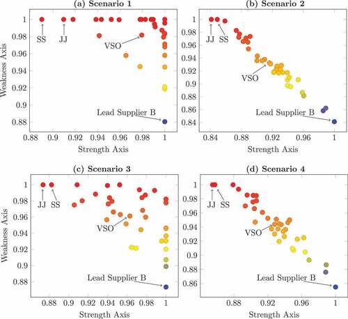
For each of the four scenarios, supplier strength (${\theta }_j^{+}$) and weakness (1/${\theta }_j^{-}$) scores are combined to generate a performance quadrant in which suppliers falling into quadrant Q1 have above-average scores on both strength and weakness dimensions. Those in Q2 have above-average scores on the strength dimension but below-average score on the weakness dimension, whilst those in Q3 have below-average scores on both the strength and weakness dimensions. Finally, suppliers plotting into Q4 have below-average scores on the strength dimension and above-average scores on the weakness dimension.

The performance-quadrant boundaries and where each supplier falls within each quadrant are a function of the location of the quadrants’ origin, known as the vendor set origin (VSO). The VSO is the coordinate location of the mean values of the strength (${\theta }_j^{+}$) and weakness (1/${\theta }_j^{-}$) scores for all suppliers. The perfect vendor location (PVL) is at the coordinate (1,0). Therefore, moving from the VSO, suppliers to the right of the vertical axis are above the mean performance for the group based on supplier strengths, whilst suppliers below the horizontal axis are “above” the mean based on supplier weaknesses. Suppliers “above” the mean on the weakness dimension are relatively stronger on their weaker factors than others located above the horizontal axis. Performance quadrants for each of the scenarios discussed below are presented in Figure 1.

Figure 1. Performance quadrants for Scenarios 1, 2, 3 and 4.

The distance that the j-th supplier is away from the PVL is given by

(7) ${\beta }_j=\sqrt{{(1-{\theta }_j^{+})}^2+{(1/{\theta }_j^{-})}^2},$(7)

where ($1-{\theta }_j^{+}$) and ($1/{\theta }_j^{-}$) are the amounts of improvement required on the strength and weakness dimensions, respectively, for the supplier to reach the PVL. A group leader, known as the lead supplier (LS), is the one with the least amount of required improvement, that is, the supplier with the minimum ${\beta }_j$, whose performance can serve as a goal for other suppliers in the set. A set of preferred, or better-performing, suppliers are those with the smaller improvement distances ${\beta }_j$. Also, the Euclidean distance between any two suppliers, for example, the lead suppliers and any other supplier, is the amount of strength and weakness improvement required by the supplier to reach the performance level of the lead supplier.

In practice, the focus and improvement-requirement goals established for any supplier may be jointly determined and agreed to by each dyad partner. Desired improvement in the j-th supplier’s strength score (${\theta }_j^{+}$) and weakness score ($1/{\theta }_j^{-}$) is referenced to the lead supplier’s (LS) scores (${\theta }_{LS}^{+}$) and ($1/{\theta }_{LS}^{-}$) and is defined as (${\theta }_{LS}^{+}$ – ${\theta }_j^{+}$) and [($1/{\theta }_j^{-}$) – ($1/{\theta }_{LS}^{-}$)], respectively. The LS scores are potentially attainable performance levels for any supplier; thus, improvement-requirement goals referenced to these scores would be realistic, as opposed to goals referenced to the PVL, which would be idealistic or “stretch” goals. The improvement distance for the j-th supplier referenced to the position of the LS is given by Equation 8(8) ${\beta }_j=\sqrt{{({\theta }_{LS}^{+}-{\theta }_j^{+})}^2+{(1/{\theta }_j^{-}-1/{\theta }_{LS}^{-})}^2}.$(8) , where the coordinates of the PVL from Equation 7(7) ${\beta }_j=\sqrt{{(1-{\theta }_j^{+})}^2+{(1/{\theta }_j^{-})}^2},$(7) are replaced by those of the LS,

(8) ${\beta }_j=\sqrt{{({\theta }_{LS}^{+}-{\theta }_j^{+})}^2+{(1/{\theta }_j^{-}-1/{\theta }_{LS}^{-})}^2}.$(8)

In other words, it is the supplier’s priority to work towards the idealistic goal of becoming or “mimicking” the perfect vendor or the more realisable goal of developing the requisite capabilities, knowledge and skills demonstrated by the leading supplier organisation (Carr et al., 2008).

For Scenario 1 (and all cases), the performance quadrant location (${\theta }_j^{+}$, $1/{\theta }_j^{-}$) for each supplier and the VSO (mean values of the strength and weakness scores) for the supplier set are presented at the bottom of Table 2 and the LS (Supplier B) is highlighted. Each supplier’s improvement distance to the LS and the mean and standard deviation of the improvement distances (${\beta }_j$) to the LS location are presented in Table 3. Top five suppliers that are closest to the lead supplier (Supplier B) are highlighted with the * sign in Table 3.

Table 3. Improvement distance to lead supplier (B) by scenario.

Supplier*	Scenario 1	Scenario 2	Scenario 3	Scenario 4
A	0.1201	0.1425	0.1235	0.126
B*	0	0	0	0
C*	0.0638	0.0825	0.0572	0.0719
D*	0.0382	0.0564	0.0255	0.0494
E	0.1215	0.1831	0.1012	0.1622
F	0.0875	0.0612	0.0604	0.0613
G	0.1195	0.1015	0.1159	0.1093
H	0.1028	0.0803	0.0469	0.0793
J	0.1195	0.0974	0.109	0.1074
K	0.1069	0.0784	0.1075	0.0744
M	0.0988	0.089	0.0979	0.0936
N	0.1201	0.1714	0.1135	0.1598
P	0.1213	0.1322	0.1359	0.1365
Q	0.1195	0.1113	0.073	0.1006
R*	0.0406	0.0223	0.0338	0.0241
U	0.1344	0.2107	0.1561	0.1888
V	0.1152	0.1241	0.1043	0.1188
W	0.1199	0.133	0.1188	0.1119
X	0.1033	0.1045	0.089	0.1001
Y*	0.0775	0.0901	0.057	0.0815
Z	0.1449	0.1584	0.1372	0.1567
AA	0.0848	0.1098	0.0883	0.104
BB	0.1259	0.1712	0.1031	0.1467
CC	0.1195	0.107	0.1202	0.1117
DD	0.1112	0.1138	0.0755	0.1068
EE	0.1163	0.1377	0.1386	0.1322
FF*	0.0681	0.1096	0.0571	0.0927
GG	0.0907	0.0237	0.0726	0.0334
HH	0.1323	0.1666	0.1248	0.167
JJ	0.1499	0.2246	0.1788	0.205
KK	0.1195	0.111	0.0633	0.1095
LL	0.1208	0.18	0.1353	0.155
MM	0.1146	0.173	0.1198	0.1539
NN	0.1287	0.1901	0.1394	0.1798
SS	0.1624	0.2193	0.1728	0.2032
$\mu$	0.1063	0.1219	0.0987	0.1147
$\sigma$	0.0324	0.0543	0.0407	0.0484
$\mathbf{m}\mathbf{i}\mathbf{n}$	0	0	0	0
$\mathbf{m}\mathbf{a}\mathbf{x}$	0.1624	0.2246	0.1788	0.205
$\mathbf{h}\mathbf{a}\mathbf{l}\mathbf{f}\mathbf{-}\mathbf{r}\mathbf{a}\mathbf{n}\mathbf{g}\mathbf{e}$	0.0812	0.1123	0.0894	0.1025

4.1.2. Scenario 1 results

As stated previously, in this scenario, the supplier evaluation considers all factors equally. This might be called a “greedy” view. It is the least-restrictive quantitative analysis and yields not only the highest average strength scores but also the highest average weakness scores of all scenarios. In Figure 1(a), 14 suppliers (40%) are considered efficient on the strength frontier, but an even larger number (17 or 48.6%) of suppliers are also on the weakness frontier. The VSO (.9794, .9817) in Table 2 is closer to both frontiers than for all the scenarios. It yields the most favourable strength scores and most unfavourable weakness scores. As a result, it is difficult for the buyer to differentiate performance amongst several ostensibly top-quality suppliers. Also, there is no assurance that the buyer’s performance factor priorities have an appropriate influence on the determination of these efficiency scores. For these two reasons, Scenario 1 suggests that the supplier evaluation process cannot be left to an approach that ignores buyer priorities and focuses heavily on just supplier performance results. This leads to the following scenarios, in which the data is weighted according to buyer preferences and top-rated suppliers’ priorities.

4.2. Scenario 2: composite of buyer’s factor priorities

4.2.1. Scenario 2 overview

Scenario 2 considers the ways that a team of evaluating buyers might value various performance factors over others. Its assurance regions serve as indicators of these evaluators’ priorities. The ranges in these regions are unilaterally determined, in that they do not consider suppliers’ priorities. The resulting information is used to evaluate the suppliers. Likewise, the strengths-and-weaknesses models used in Scenario 1 are modified to include the evaluator’s preferences as assurance regions for Scenario 2, where the strength model is

Strength $Mode{l}_j$:

(9) $\hspace{0.17em}Maximize\hspace{0.17em}{\theta }_j^{+}=\sum _{i=1}^n{u}_{i,j}.S_{i,j},$(9)

(10) $s.t.\hspace{0.17em}\sum _{i=1}^n{u}_{i,j}.S_{i,j}\le 1\hspace{0.17em},\mathrm{\forall }\hspace{0.17em}j,$(10)

(11) $L_{i,i+1}\le (u_{i,j}/u_{i+1,j})\le U_{i,i+1}\hspace{0.17em},\mathrm{\forall }\hspace{0.17em}i\in \{1,\dots ,n-1\},$(11)

(12) $u_{i,j}\ge 0\hspace{0.17em},\mathrm{\forall }\hspace{0.17em}i,j;$(12)

The weakness model is stated as

Weakness $Mode{l}_j$:

(13) $\hspace{0.17em}Minimize\hspace{0.17em}{\theta }_j^{-}=\sum _{i=1}^n{u}_{i,j}.S_{i,j},$(13)

(14) $s.t.\sum _{i=1}^n{u}_{i,j}.S_{i,j}\ge 1,\mathrm{\forall }j,$(14)

(15) $L_{i,i+1}\le (u_{i,j}/u_{i+1,j})\le U_{i,i+1}\hspace{0.17em},\mathrm{\forall }\hspace{0.17em}i\in \{1,\dots ,n-1\},$(15)

(16) $u_{i,j}\ge 0\hspace{0.17em},\mathrm{\forall }\hspace{0.17em}i,j.$(16)

In this scenario, the strengths-and-weaknesses models are weighted to reflect each supplier’s preferences by maximising ${\theta }_j^{+}$ in the strength model and minimising ${\theta }_j^{-}$ in the weakness model. This is done by adjusting the constraints (Equations (10)(10) $s.t.\hspace{0.17em}\sum _{i=1}^n{u}_{i,j}.S_{i,j}\le 1\hspace{0.17em},\mathrm{\forall }\hspace{0.17em}j,$(10) and (14(14) $s.t.\sum _{i=1}^n{u}_{i,j}.S_{i,j}\ge 1,\mathrm{\forall }j,$(14) ), respectively) in each model to ensure that the weight values are between zero and one and that the assurance region constraints (Equations (11)(11) $L_{i,i+1}\le (u_{i,j}/u_{i+1,j})\le U_{i,i+1}\hspace{0.17em},\mathrm{\forall }\hspace{0.17em}i\in \{1,\dots ,n-1\},$(11) and (15(15) $L_{i,i+1}\le (u_{i,j}/u_{i+1,j})\le U_{i,i+1}\hspace{0.17em},\mathrm{\forall }\hspace{0.17em}i\in \{1,\dots ,n-1\},$(15) ), respectively) in each model so that the weights ($u_{i,j}$) reflect the buyer’s priorities.

The ratio $(u_{i,j}/u_{i+1,j})$ in each model formulation expresses the relative weight value of the i-th factor compared to each of the other factors for the j-th supplier, and creates the assurance regions defined by the lower $(L_{i,i+1})$ and upper $(U_{i,i+1})$ bounds. These bounds integrate evaluators’ preferences. They also capture the diversity in those preferences and ensure that the input provided by these evaluators is considered more evenly when creating the decision variable weights $(u_{i,j})$ that determine the efficiency score of the supplier.

The assurance-region bounds of Equations (11)(11) $L_{i,i+1}\le (u_{i,j}/u_{i+1,j})\le U_{i,i+1}\hspace{0.17em},\mathrm{\forall }\hspace{0.17em}i\in \{1,\dots ,n-1\},$(11) and (15(15) $L_{i,i+1}\le (u_{i,j}/u_{i+1,j})\le U_{i,i+1}\hspace{0.17em},\mathrm{\forall }\hspace{0.17em}i\in \{1,\dots ,n-1\},$(15) ) reflect the buyer-evaluation team members’ priorities for the performance factors and are formed as follows: First, for the k-th evaluator, all weight ratios are determined for each pair of factors comprising the performance scorecard. For example, $(W_1/W_2{)}_k$ is the ratio of the first and second performance factor weights assigned by the k-th evaluator. Second, the minimum and maximum weight ratios of the first and second factors, across all evaluators on the team, are determined. These are called $L_{12}$ and $U_{12}$, respectively. Together, these weight bounds reflect the underlying preference scores of the evaluation team. Table 4 – Panel A summarises the preferred ranges for Scenario 2, and for the remaining scenarios, that will be discussed.

Table 4. Defined assurance regions.

Panel A: Assurance region bounds for attribute ratios
Attribute Ratio		Scenario 2		Scenario 3		Scenario 4
Numerator	Denominator	Min	Max	Min	Max	Min	Max
CST56	CST55	0.67	1.29	0.00	1.01	0.67	1.91
CST57	CST55	0.56	0.93	0.00	9.62	0.56	1.67
OTS	CST55	0.56	1.08	0.12	2.49	0.56	2.12
OTD	CST55	0.50	1.15	0.12	2.35	0.50	1.80
ACCEPT	CST55	0.76	1.00	0.13	21.23	0.76	1.72
CST57	CST56	0.67	0.83	0.00	9.56	0.67	1.15
OTS	CST56	0.44	1.17	1.00	2.47	0.44	1.90
OTD	CST56	0.47	1.25	1.00	6.86	0.47	2.81
ACCEPT	CST56	0.67	1.33	1.02	26.88	0.67	3.31
OTS	CST57	0.62	1.75	0.10	1.10	0.62	2.88
OTD	CST57	0.58	1.88	0.00	6.85	0.58	4.48
ACCEPT	CST57	0.92	1.63	0.19	21.06	0.92	3.05
OTD	OTS	0.47	1.25	0.00	6.86	0.47	2.81
ACCEPT	OTS	0.80	1.60	0.67	26.88	0.80	4.00
ACCEPT	OTD	0.87	1.78	0.15	26.96	0.87	4.51
Panel B: Region range and class for attribute ratios
Attribute Ratio		Scenario 2		Scenario 3		Scenario 4
Numerator	Denominator	Range	Class^a	Range	Class^a	Range	Class^a
CST56	CST55	0.62	M	1.01	C	1.24	M
CST57	CST55	0.37	C	9.62	M	1.11	C
OTS	CST55	0.52	C	2.36	M	1.56	M
OTD	CST55	0.65	M	2.23	C	1.30	C
ACCEPT	CST55	0.24	C	21.10	D	0.96	C
CST57	CST56	0.16	C	9.56	M	0.48	C
OTS	CST56	0.73	M	1.47	C	1.46	M
OTD	CST56	0.78	M	5.87	M	2.34	M
ACCEPT	CST56	0.66	M	25.86	D	2.64	D
OTS	CST57	1.13	D	1.00	C	2.26	M
OTD	CST57	1.30	D	6.85	M	3.90	D
ACCEPT	CST57	0.71	M	20.87	M	2.13	M
OTD	OTS	0.78	M	6.86	M	2.34	M
ACCEPT	OTS	0.80	D	26.21	D	3.20	D
ACCEPT	OTD	0.91	D	26.81	D	3.64	D

^aC for conforming below the 1st quartile, M for mediating between the 1st and 3rd quartiles and D for disparate above the 3rd quartile.

The preferred ranges are given by three classifications in Table 4 – Panel B: Conformity (C), Mediation (M) and Disparity (D). Conformity indicates that the evaluators generally agreed about the relative weight of the factor and assigned similar values, so that the range ($U_{ij}-L_{ij}$) is narrow. Alternately, some of the weight ratios show disparity amongst the evaluators regarding the importance of a factor (the numerator) relative to another (the denominator).

4.2.2. Scenario 2 results

The results of this scenario suggest that this framework provides the buyer with a clear focus on its own priorities amongst the six supplier-performance factors, but does not account for the suppliers’ own environments and capacities. Adding the buyer’s priority information as a weight factor in Scenario 2 is shown to reduce suppliers’ strength efficiency scores. The strength and weakness results for each supplier and the VSO (.9176, .9309) are presented in Table 2, whilst the lead supplier (LS) and mean and standard deviation of the improvement distances to the LS are presented in Table 3.

Compared to Scenario 1, the priorities used to weight this scenario impose restrictions on the data, reducing both the average strength and weakness scores according to the VSO (.9176, .9309) reported in Table 2. This table’s reduction of the weakness score, with a positive movement away from the weakness frontier, improves its assessment of the weaker performance scores. Equipped with this directed information, buying firms can more effectively stratify the performances of various suppliers. For example, a first glance at the data plot in Figure 1(b) suggests that only one supplier (B) lies on the strength frontier and that only two suppliers (JJ and SS) lie on the weakness frontier. In Table 3, the Scenario 1 average improvement distance (${\beta }_j$) to the LS is 0.1063 for the supplier set, whilst the average is 0.1219 for Scenario 2. Comparatively, the supplier set results in Scenario 2 are located farther away from its lead supplier. The dispersion in the improvement distances to the LS is also greater in Scenario 2 (.0543) than in Scenario 1 (.0324). However, the stratification pattern depicted in Figure 1(b) (Scenario 2) provides a clearer view of relative supplier performance than in Figure 1(a) (Scenario 1). This scenario demonstrates a situation in which the buyer evaluates relative supplier performance using its strictest set of guidelines, thereby lowering scores for both the average strength and weakness scores reported for Scenario 2.

But the universality of these guidelines is, of course, limited by idiosyncrasies such as the supplier’s internal operating environment and the unique market environment between a supplier and buyer. The improvement guidelines developed here are unilateral. The Scenario 2 approach grants discriminatory power entirely to the buyer. It does not account for the ways that these factors will impact suppliers’ capabilities. It is a more tightly constrained evaluation of suppliers’ strengths, whilst relaxing the evaluation of supplier weaknesses.

4.3. Scenario 3: composite of top-rated suppliers’ priorities

4.3.1. Scenario 3 overview

Scenario three considers suppliers’ capability to address the priorities expressed by the top-rated suppliers. This scenario implies that the buyer defers the priorities of the evaluation to this group. For role-model suppliers, their performance reflects the potential capabilities of the entire supplier set. Therefore, in this case, supplier capabilities were measured using a subset of preferred suppliers who set the performance standards.

First, the results of the strength models from Scenario 1 are used to designate the top-rated suppliers. The bottom of Table 3 presents the minimum, maximum and half-range of improvement distances to the LS for each scenario. Suppliers were designated “top-rated” if their improvement distance (${\beta }_j$) to the lead supplier (LS) is less than the half-range of the improvement distances for all suppliers in the set (a proximity measure). As before, the corresponding factor weights are then used to construct assurance regions. The top-rated suppliers and their respective improvement distances to the LS were first identified in Table 3 and summarised in Table 5.

Table 5. DEA weights for attributes of the preferred suppliers from scenario 1.

Preferred Suppliers	CST55	CST56	CST57	OTS	OTD	ACCEPT
B	0.0026	0.0003	0.0000	0.0003	0.0003	0.0086
D	0.0004	0.0004	0.0036	0.0004	0.0009	0.0053
R	0.0007	0.0007	0.0061	0.0017	0.0007	0.0011
C	0.0004	0.0000	0.0005	0.0004	0.0004	0.0095
FF	0.0000	0.0000	0.0005	0.0006	0.0000	0.0094
Y	0.0045	0.0006	0.0006	0.0006	0.0040	0.0006

Next, the strength model results from Scenario 1 are used to develop the DEA weights for Scenario 3. Table 5 shows these results. Note that weakness model results could not be incorporated because these results assign weights to indicate the lower-performing factors, meaning that the strongest performance factors for the top-rated suppliers would be assigned low or zero weights to minimise their weakness efficiency score. For this reason, using weights from the weakness model in this scenario would contradict the objective of the study and thus confuse the differentiation between the higher- and lower-performing suppliers. In the case of a zero weight, the results could falsely indicate that a performance factor is irrelevant and should be ignored.

As in the previous scenarios, the weights ($u_{i,j}$) determined by this process are used to form the assurance regions. This is achieved using the minimum and maximum values of the ratios of weights for each pair of factors across all preferred suppliers. These assurance-region bounds for Scenario 3, as presented in Table 4 – Panel A, replace the corresponding bounds used in Scenario 2 from the buyer evaluation team. Once again, the ratio bounds, depending on their range, are labelled Conforming (C) when below the first quartile, Mediating (M) when in the inner-quartile range, or disparate (D) when greater than the third quartile. These range classes are presented in Table 4 – Panel B.

After the weights and assurance regions are determined, an input-oriented strengths-and-weaknesses efficiency model, as shown in Equations 9(9) $\hspace{0.17em}Maximize\hspace{0.17em}{\theta }_j^{+}=\sum _{i=1}^n{u}_{i,j}.S_{i,j},$(9) through 16(16) $u_{i,j}\ge 0\hspace{0.17em},\mathrm{\forall }\hspace{0.17em}i,j.$(16) , evaluated the supplier set. The strengths-and-weaknesses supplier scores, the VSO, and the LS, are all presented in Table 2. This table shows that the VSO (.9629, .9613) in Table 2 falls between that for Scenario 1 and Scenario 2.

4.3.2. Scenario 3 results

This scenario is most useful in determining an attainable or reasonable set of improvement goals for suppliers. It offers a more relaxed set of priority levels than Scenario 2. Furthermore, it is more useful than Scenario 1, but less useful than Scenario 2, in differentiating amongst supplier performances. For a buyer, this scenario can help to establish a credible foundation for their priorities because all suppliers are plotted closer to the LS (see Figure 1(c)).

Because this scenario allows top-rated suppliers’ capabilities to determine the priority settings, it provides results reflecting a more realistic set of priorities. By considering the improvement distances from the LS, as presented in Table 3, we can see that the average improvement distance to the LS (.0987) is less than those of either Scenario 1 or Scenario 2, indicating that the average supplier has received a rating closer to that of the top-rated suppliers. It is also shown that the dispersion of improvement distances (.0407) is greater than that of Scenario 1 but less than that of Scenario 2. This indicates that the supplier set is now clustered closer to the LS than it was in Scenario 2.

The performance quadrants for this scenario appear in Figure 1(c). They reveal that using top-rated suppliers’ priority weights can assist in differentiating amongst supplier performances, but are less useful in this capacity than were the weights assigned in Scenario 2. By deferring to these weights, fewer strength-efficient suppliers (10, or 28.6%) and also fewer weakness-inefficient suppliers (4 or 11.4%) emerge than were present in Scenario 1.

4.4. Scenario 4: composite of buyer preferences and top-rated supplier priorities (bilateral ranges)

4.4.1. Scenario 4 overview

This fourth scenario considers both the buyer’s preferences and the top-rated suppliers’ priorities, as if the evaluators met with executives at these supply firms to jointly rank these factors. Scenario 4 uses the ratio bounds specified and determined by both the buyer evaluation team (per Scenario 2) and the top-rated suppliers (per Scenario 3). This is accomplished by using the buyer’s (Scenario 2) range as a base range, and then adjusting each factor’s upper bound ($u_{i,j}$) according to whether it was categorised as conforming, mediating, or diverging in the top-rated suppliers’ range (Scenario 3). Accordingly, in cases where the top-rated suppliers’ range is conforming, the buyer’s range (per Scenario 2) was doubled. When the suppliers’ range is mediating, the base range is tripled. If the suppliers’ range is disparate, the base range is quadrupled. As in the preceding cases, Scenario 4 uses Equations 9(9) $\hspace{0.17em}Maximize\hspace{0.17em}{\theta }_j^{+}=\sum _{i=1}^n{u}_{i,j}.S_{i,j},$(9) through 16(16) $u_{i,j}\ge 0\hspace{0.17em},\mathrm{\forall }\hspace{0.17em}i,j.$(16) to create the ratio-bounds. These enlarged ranges and their magnitude of enlargement, in Scenario 4, reflect the dispersion of the weights achieved under Scenario 3. The more conforming the suppliers’ range under Scenario 3, we need a smaller range for the bilateral weight adjustments under Scenario 4. The greater the dispersion in supplier’s range under Scenario 4, we utilise a broader range to reflect the potential dispersion in supplier weights. The resulting ranges for Scenario 4 are presented in Table 4 – Panel A, along with the classification of the ranges in Table 4 – Panel B.

As in the preceding cases, Scenario 4 uses Equations 9(9) $\hspace{0.17em}Maximize\hspace{0.17em}{\theta }_j^{+}=\sum _{i=1}^n{u}_{i,j}.S_{i,j},$(9) through 16(16) $u_{i,j}\ge 0\hspace{0.17em},\mathrm{\forall }\hspace{0.17em}i,j.$(16) to create ratio bounds labelled (C), (M) or (D). The difference in this situation is that they are bilaterally determined. Conceptually, there can be many alternative methods to develop the ranges chosen for our purposes here. However, care must be taken to avoid non-feasible solutions resulting from lower bounds that are too high, zero-value lower bounds for factor ratios (given that these will falsely indicate non-importance) and order-of-magnitude differences between buyer and supplier ratio bounds.

4.4.2. Scenario 4 results

This scenario balances the buyers’ preferences and suppliers’ priorities. Of the four scenarios, it is therefore the most representative of what is both desirable to buyers and realistic for suppliers. Because the assurance ranges in Scenario 4 are doubled, tripled or quadrupled from those of Scenario 2 (according to the factors’ (C), (M) or (D) statuses in Scenario 3), they represent a more relaxed set of buyer priorities on the strength axis (See Figure 1(d)). Not surprisingly, the bilateral compromise on priorities increased (improved) the average strength score (.9281) over the average strength score in Scenario 2 (.9176). Furthermore, the standards for evaluating weaknesses are more relaxed than those of Scenario 3, and this leads to a decrease (improvement) in the average weakness score (.9439), as opposed to .9613 in Scenario 3. It is also shown that both the average improvement distance to the LS (.1147) and the variability (.0484) of these distances, as shown in Table 3, are less than those in Scenario 2, but greater than those in Scenario 3. This represents a closer and tighter clustering of supplier locations to the LS than that for the unilateral buyer-priority case (Scenario 2), but a looser cluster than if the goals are set only by top-rated suppliers (Scenario 3).

The following conclusions can be drawn regarding Scenario 4. In cases where an assurance-region range is conforming, meaning that the factor weights ($u_{i,j}$) of the top-rated suppliers are consistent, the assurance regions of Scenario 4 place more critical emphasis on suppliers’ strengths. Conversely, with disparate ranges in which factor weights are inconsistent, the feasible region expands to place critical emphasis on suppliers’ weaknesses. Finally, in cases with mediating ranges, less emphasis is placed on strengths, and more is placed on weaknesses. The scoring results for Scenario 4 are also shown in Tables 2 and 3.

5. Discussion

In summary, the sequence of case scenarios represented suggests a transition away from the traditional unilaterally focused supplier evaluations: This study offers four scenarios that culminate in a more bilateral approach; the first based strictly on consideration of the supplier performance factors (Scenario 1); the second based on using buyer imposed performance factor priorities to evaluate supplier performance (Scenario 2); the third (Scenario 3) represents the intermediate step of determining what the supplier set is capable of as reflected in the performance of a set of top-rated suppliers and how this is used to evaluate supplier performance and the fourth (Scenario 4) reflects cooperation in an evaluation environment featuring a supplier-capability- and a buyer-priority-based analysis. A discussion of specific benefits for buyers and suppliers follows in this section.

5.1. Buying firms: value of the bilateral DEA method

The method demonstrated here can help buyers who seek improvements from inefficient supply-chain partners. First, DEA analysis revealed the importance of accounting for multifarious dimensions of performance. The process identifies performance references on strengths and weaknesses in the form of a vendor set origin. This leads to identifying top-rated organisations that can act as role models for inefficient units. This is in fact very relevant to top managers of today’s firms, who have multiple units and service multiple markets (MUMM). This method allows corporate executives of MUMM organisations to use existing information from their respective organisation units and, at a fairly low cost, employ the methods used in the present study to identify inefficient units, assign suitable role models and thus improve the likelihood of transferring best practices through developing suppliers.

The results of this study demonstrate the value of this method for buyers. Consider the bilateral priority ranges from Scenario 4. Table 6 – Panel A presents the buyer’s priority rank for each performance factor, and the frequency that the factor is the highest weighted factor for suppliers requiring strength improvement to reach the performance level of the leader supplier, whilst Table 6 – Panel B does the same for suppliers requiring weakness improvement. Regarding supplier strength improvement, only 22.9% of suppliers requiring improvement have the buyer’s highest priority factor as their strongest factor, whilst 48.6% and 11.4% of suppliers requiring strength improvement have the buyer’s two lowest priority factors as their strongest factor, respectively. Clearly, in the latter case, this situation requires buyer intervention to redirect the supplier’s improvement efforts towards factors that are of higher priority to the buyer. Furthermore, when excluding all priority information (Scenario 1), the analysis found only 14 of 35 suppliers to be strength efficient and that for both strengths and weaknesses, the suppliers’ strongest factors tended to be uniformly distributed across all factors (except CST57 for strengths). Moreover, the weakness dimensions in Table 6 – Panel B demonstrate that a significant number of suppliers (26.5% and 47.1%), if simply working to improve on their weakest factor, would actually be focusing their efforts on the buyer’s two factors of lowest priority. For 17.6% of these suppliers, their weakest area is the buyer’s highest-priority factor. However, with the bilateral DEA approach demonstrated here, a buyer will be able to reinforce the improvement efforts of the suppliers, thereby building some consistency between their own foci and the suppliers’. By using this buyer priority information in the DEA model, we suggest that the buyer now has supplier performance data with which to justify and then direct supplier improvement efforts. A second major contribution of this study’s approach to performance evaluation and selection is to enhance buyers’ discrimination of performance amongst inefficient supplier organisations. This discriminatory power evolves, in part, from the way that our process encourages buyers and suppliers to communicate their expectations. For example, consider the efficiency scores in all four scenarios, as reported in Table 2. For the sub-group of inefficient suppliers, there are differences worth noting. The average scores for the inefficient suppliers in Scenarios 3 and 4 (0.9481/0.9259 for strengths; 0.956/0.938 for weakness, respectively) improve the ability to discriminate suppliers’ relative performance. That is, suppliers classified as inefficient via the maximally flexible, unbounded approach in Scenario 1 are generally truly inefficient. Thus, the lower average scores of ensuing Scenarios 3 and 4 have now provided more clarity amongst the suppliers’ strength and weakness capability.

Table 6. Strength/weakness improvement.

Panel A
Factor	Buyer Rank	Scenario 1	Scenario 4
ACCEPT	1	23.8%	22.9%
CST55	2	19.0%	8.6%
CST56	3	14.3%	5.7%
CST57	4	0.0%	2.9%
OTS	5	14.3%	11.4%
OTD	6	28.6%	48.6%
Panel B
Factor	Buyer Rank	Scenario 1	Scenario 4
ACCEPT	1	17.6%	17.6%
CST55	2	5.9%	0.0%
CST56	3	17.6%	8.8%
CST57	4	14.7%	0.0%
OTS	5	29.4%	47.1%
OTD	6	14.7%	26.5%

Of course, the buyers themselves must decide how to act upon these data regarding their existing supply chain partners. In the spirit of enhancing discriminatory power, this dual strength/weakness approach provides results that can be used to develop a set of performance-improvement prescriptions. These guidelines result in the ability to now communicate to suppliers not only a performance role model in the form of a lead supplier but also a set of recommendations about which dimensions of performance require development focus by the supplier. We incorporated the notion of required effort or distance cost by determining the distance between the low-performing supplier and the lead supplier. This has important implications for the buyer in terms of deciding how its own supplier development resources should be best allocated when collaborating with suppliers in this capacity. Nevertheless, it is now possible to decide which improvement levers to enact and to do so with both a short-term and long-term orientation as desired.

5.2. Supplying firms: value of the bilateral DEA method

But what effect does buyer priority information have on the improvement focus taken by the supplier? This question is central to the discussion of supplier performance improvement (or development). Because this method combines the preferences of buyers with the priorities of top-rated suppliers, it can allow them to make educated choices about how they will improve their operations. Without the incorporation of information from the buyer’s priorities, suppliers requiring improvement will likely myopically focus their efforts on attributes that are easiest or least costly to improve. Alternately, the buyers might direct the supplier to focus its behaviours on improvement on their own high-priority attributes, but doing so may not necessarily translate into higher levels of overall success for the supplier.

To demonstrate the effects that priority information has on the improvement direction, we compared the DEA results from Scenario 1 (no buyer priority information) with those of Scenario 4 (bilateral priority ranges). As mentioned previously, the solutions of the DEA models in Scenario 1 and Scenario 4 for each supplier include strength scores (${\theta }_j^{+}$) and weakness scores (1/${\theta }_j^{-}$), as well as the weights ($u_{ij}$) placed on each performance factor to achieve their respective scores. For the strength model, the supplier’s strongest factor receives the highest weight value, whilst for the weakness model, the supplier’s weakest factor receives the highest weight value. Any supplier can improve its performance on any factor to achieve the performance level of a lead supplier (LS), but it is DEA efficient for that supplier to direct its attention to improvement on the factor with the highest value DEA weight.

6. Conclusions

This study provides a framework for evaluating suppliers’ performance according to the preferences of buyers and/or the priorities of top-rated suppliers. The framework tested here serves the important goal of incorporating managerial preferences into the supplier evaluation process. It also extends the discussion towards perspectives on developing suppliers using performance improvement frontiers that we constructed here. Several previous studies reviewed in this paper emphasised a primary goal of rationalising suppliers based on performance. The goal of these studies was to derive performance improvement plans for each supplier and recommended plans that the buyer should enact to improve its performance and reduce “buyer shirking” of the suppliers. The current paper, however, extends these efforts using scenarios 2–4 as discussed in the paper to offer bilateral linkages between the buyer preferences and its top-rated suppliers as new goal posts for performance improvement. As a novel contribution to the literature, we now contend that suppliers’ capabilities are bounded by the priority weights of the best competing suppliers and that this should be blended with the buyer survey-generated approach, thus representing a compromise between buyer wants and supplier capabilities.

The analyses demonstrated here also represent effective frameworks for suppliers to model inefficiencies in organisational units and to identify best practice role models, whilst still allowing the model to adapt to changes in subjective preferences. As stated earlier, this study builds on prior published papers that take a DEA-based approach. We use both a maximising and minimising DEA objective function in order to use both strength and weakness models. With this view in mind, it becomes possible to graph suppliers’ performance according to their efficiency scores across both functions.

6.1. Limitations and future research directions

One limitation in this study is the fact that it offers only a cross-section, limited to data from one organisation. Because this framework serves a dynamic context, it was not our goal to provide a universal set of best-practice templates. Instead, it allows a firm to link the recommended actions to performance changes and to supply base development instead of simply pruning. Of course, in the long term, many partners exit relationships, however. Our results allow for the creation of new pools of role models for a specific point in time and allow firms to change their best-practice templates according to fluctuations in the market and the firm’s own business situation. Specifying templates may require the use of other methodologies and comparison lying beyond our scope here, but should be left to future work.

A logical extension to this study might be an analysis of supplier evaluation and development over the life cycle of an organisation or relationship. Although it is, of course, unlikely that an organisation could eliminate all inefficiencies at the unit level, our analysis may help suppliers to keep shortfalls in resource utilisation to a minimum, enhancing their own performance and sustaining a competitive advantage. We acknowledge that, in practice, there are institutional impediments to realising significant improvements in supplier capabilities and that some suppliers’ efforts may only be symbolic in nature. However, we leave this discussion to work appearing elsewhere. Furthermore, efficiency-improvement decisions are influenced by the nature of the data used, the shape of the efficient frontier determined by the data used, and how potential best-practice templates are identified. Further research on these topics will generate more insights for buying firms as they evaluate suppliers, and for suppliers as they work to increase their value.

Disclosure statement

No potential conflict of interest was reported by the author(s).

Appendix.

General background on data envelopment analysis models

Efficiency-based methodologies such as DEA have been used to assess performance because they have been shown to address in one comprehensive manner a large number of input and output factors (Weber & Desai, 1996). This method affords the opportunity to establish the required relative comparisons within the supplier evaluation process. Consider an example with two evaluation criteria, $Y_1$ and $Y_2$, used to evaluate supplier efficiency as illustrated in Figure A1. Each supplier’s performance is plotted along these two output dimensions and the location represents the supplier’s relative performance compared to the other suppliers. Suppliers’ relative performance on the criteria can often be constrained by characteristics of the behaving (executing) system linkages with its buying firm. This constraint forces trade-offs amongst the various criteria in use. As shown below in Figure A1, the frontier depicts the performance assessment for the combination of two criteria.

Figure A1. Performance assessment using efficiency frontiers.

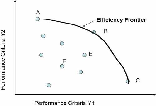
We formulate below a general DEA model for analysing supplier performance data. The data-dependent relationships in the model are also described. Assume a set of H (h = 1, 2, …, H) suppliers, evaluated on J (j = 1, 2, …, J) buyer performance inputs $z_{jh}$, M (m = 1,2,..,M) purchase control values $x_{mh}$ and I (i = 1,2,..,I) supplier performance outputs. Computationally, the model is run H times in order to compute the efficiency scores (${\theta }_k^{\ast }$) for each of the H suppliers. The model for the k-th supplier is

(A1) $Maximize\hspace{0.17em}{\theta }_k^{\ast }=\sum _{i=1}^I{u}_{ik}.y_{ik},$(A1)

(A2) $s.t.\hspace{0.17em}\sum _{m=1}^M{w}_{mk}.x_{mk}+\sum _{j=1}^J{v}_{jk}.z_{jk}=1,$(A2)

(A3) $3\sum _{i=1}^I{u}_{ih}.y_{ih}-\sum _{m=1}^M{w}_{mh}.x_{mh}-\sum _{j=1}^J{v}_{jh}.z_{jh}\le 0,\mathrm{\forall }h=1,\dots ,H,$(A3)

(A4) $u_{ik},v_{jk},w_{mk}\ge 0,$(A4)

where

• $y_{ih}$ is the observed value of the i-th output for the h-th supplier.

• $x_{mh}$ is the observed value of the m-th purchase control input variable for the h-th supplier.

• $z_{jh}$ is the observed value of the j-th buyer-related input variable for the h-th supplier.

• $y_{ik}$ is the observed value of the i-th output value observed for the k-th supplier whose performance is currently under evaluation.

• $x_{mk}$ is the the observed value of the m-th purchase control input variable for the k-th supplier whose performance is currently under evaluation.

• $z_{jk}$ is the observed value of the j-th buyer-related input variable for the k-th supplier whose performance is currently under evaluation.

• $v_{jk}$ is the the weight given to the j-th buyer-related input for the k-th supplier.

• $w_{mk}$ is the weight given to the m-th purchase control input value for the k-th supplier.

• $u_{ik}$ is the weight given to the i-th output for the k-th supplier.

Equation (A1) uses output performance attribute data for the k-th supplier and assigns a weight to each attribute that maximises the overall performance score, ${\theta }_k^{\ast }$, for that supplier. Equation (A2) uses inputs – the buyer performance attributes, $z_{jk}$, and the purchase control variables, $x_{mk}$ – to set input weights, $v_{jk}$ and $w_{mk}$, for the k-th supplier. Equation (A3) is a set of constraints that balance the input and output performance attributes such that the weighted sum of the output attributes for each supplier is limited or constrained by (is less than) the weighted sum of the input performance attributes of the buying firm and the purchase control variables for that supplier. This last term in Equation (A3) captures the impact that buying firm’s actions have on supplier performance evaluation in the dyadic relationship. Although not the focus here, the formulation provides for the potential to explicitly incorporate managers’ subjective preferences on the DEA weights.

By maximising Equation (A1) subject to the constraints A2 – A3, one assigns the most preferable weight set to the k-th supplier so that the strengths of the k-th supplier are evaluated. Simultaneously, the same weight set is utilised to evaluate all other suppliers in comparison to the target supplier. The k-th supplier with (θ_k* = 1.0) is considered to be efficient, whilst (θ_k* < 1.0) suggests that the k-th supplier is inefficient. Specifically, Charnes et al. (1978) define “CCR-efficiency” as follows: the k-th supplier is CCR-efficient if (θ_k* = 1.0) and there exists at least one optimal set of weights (v*,u*), with v* > 0 and u* > 0. Otherwise, the k-th supplier is CCR-inefficient, meaning that either (θ_k* <1.0) or that (θ_k* = 1.0) and at least one element of (v*,u*) is zero for every optimal solution of the CCR model. DEA efficiency is a robust tool for performance evaluation because it is based on the ratio of inputs to outputs that form the empirical production frontier (Charnes et al., 1997).

In terms of solving the DEA model, there is a six-decade history; Tone (2001) and Cooper et al. (2006) reviewed prior, and then introduced new, solution methodologies reported elsewhere. Because DEA employs a piece-wise linear frontier comprising the efficient decision-making units (DMUs) in the data set, any inefficient unit is inefficient only with respect to the DMUs in its reference set (Banker et al., 1984). This now ensures that subsequent use of the resulting efficiency scores is accomplished more equitably and without regard to the units of measure assigned to the variables (unit invariant such as monetary value, proportions, distances, etc.). We maximise Equation (A1) subject to the constraints in Equations (A2) through (A4). This results in a set of efficiency scores for the supplier set and they are used to explore performance.

References

- Andersson, U., Forsgren, M., & Holm, U. (2002). The strategic impact of external networks: Subsidiary performance and competence development in the multinational corporation. Strategic Management Journal, 23(11), 979–996. https://doi.org/10.1002/smj.267
- Badiezadeh, T., Saen, R. F., & Samavati, T. (2018). Assessing sustainability of supply chains by double frontier network dea: A big data approach. Computers & Operations Research, 98(10), 284–290. https://doi.org/10.1016/j.cor.2017.06.003.
- Banerjee, A., Roychoudhury, B., & Gogoi, B. J. (2020). Determining rank in the market using a neutrosophic decision support system. Journal of Business Analytics, 3(2), 138–157. https://doi.org/10.1080/2573234X.2020.1834883
- Banker, R. D., Charnes, A., & Cooper, W. W. (1984). Some models for estimating technical and scale inefficiencies in data envelopment analysis. Management Science, 30(9), 1078–1092. https://doi.org/10.1287/mnsc.30.9.1078
- Barry, J. M., Dion, P., & Johnson, W. (2008). A cross-cultural examination of relationship strength in b2b services. Journal of Services Marketing, 22(2), 114–135. https://doi.org/10.1108/08876040810862868
- Braglia, M., & Petroni, A. (2000). A quality assurance-oriented methodology for handling trade-offs in supplier selection. International Journal of Physical Distribution & Logistics Management, 30(2), 96–112. https://doi.org/10.1108/09600030010318829
- Buffa, F. P., & Ross, A. D. (2011). Measuring the consequences of using diverse supplier evaluation teams: A performance frontier perspective. Journal of Business Logistics, 32(1), 55–68. https://doi.org/10.1111/j.2158-1592.2011.01005.x
- Carr, A. S., Kaynak, H., Hartley, J. L., & Ross, A. (2008). Supplier dependence: Impact on supplier’s participation and performance. International Journal of Operations & Production Management, 28(9), 899–916. https://doi.org/10.1108/01443570810895302
- Charles, V., Aparicio, J., & Zhu, J. (2021). Data science for better productivity. Journal of the Operational Research Society, 72(5), 971–974. https://doi.org/10.1080/01605682.2021.1892466
- Charles, V., Färe, R., & Grosskopf, S (2016). A translation invariant pure dea model. European Journal of Operational Research, 249(1), 390–392. https://doi.org/10.1016/j.ejor.2015.09.037
- Charnes, A., Cooper, W. W., & Rhodes, E. (1978). Measuring the efficiency of decision making units. European Journal of Operational Research, 2(6), 429–444. https://doi.org/10.1016/0377-2217(78)90138-8
- Charnes, A., Cooper, W., Lewin, A. Y., & Seiford, L. M (1997). Data envelopment analysis theory, methodology and applications. Journal of the Operational Research Society, 48(3), 332–333. https://doi.org/10.1057/palgrave.jors.2600342
- Chen, C., & Yan, H. (2011). Network dea model for supply chain performance evaluation. European Journal of Operational Research, 213(1), 147–155. https://doi.org/10.1016/j.ejor.2011.03.010
- Chen, Y., Cook, W. D., & Lim, S. (2019). Preface: Dea and its applications in operations and data analytics. Annals of Operations Research, 278(1), 1–4. https://doi.org/10.1007/s10479-019-03243-w
- Cook, W. D., Tone, K., & Zhu, J. (2014). Data envelopment analysis: Prior to choosing a model. Omega, 44(4), 1–4. https://doi.org/10.1016/j.omega.2013.09.004
- Cooper, W. W., Seiford, L. M., & Tone, K. (2006). Introduction to data envelopment analysis and its uses: With dea-solver software and references. Springer Science & Business Media.
- Day, G. S. (2000). Managing market relationships. Journal of the Academy of Marketing Science, 28(1), 24–30. https://doi.org/10.1177/0092070300281003
- Dickson, G. W. (1966). An analysis of vendor selection systems and decisions. Journal of Purchasing, 2(1), 5–17. https://doi.org/10.1111/j.1745-493X.1966.tb00818.x
- Dutta, P., Jaikumar, B., & Arora, M. S. (2021). Applications of data envelopment analysis in supplier selection between 2000 and 2020: A literature review. Annals of Operations Research, 2021:2 , 1–56. https://doi.org/10.1007/s10479-021-03931-6
- Fugate, B. S., Mentzer, J. T., & Stank, T. P. (2010). Logistics performance: Efficiency, effectiveness, and differentiation. Journal of Business Logistics, 31(1), 43–62. https://doi.org/10.1002/j.2158-1592.2010.tb00127.x
- Galagedera, D. U. A., & Silvapulle, P. (2003). Experimental evidence on robustness of data envelopment analysis. Journal of the Operational Research Society, 54(6), 654–660. https://doi.org/10.1057/palgrave.jors.2601507
- Gattorna, J., & Jones, T. (1998). Strategic supply chain alignment: Best practice in supply chain management. Gower Publishing.
- Golicic, S. L., & Mentzer, J. T. (2006). An empirical examination of relationship magnitude. Journal of Business Logistics, 27(1), 81–108. https://doi.org/10.1002/j.2158-1592.2006.tb00242.x
- Griffith, D. A., Hoppner, J. J., Lee, H. S., & Schoenherr, T. (2017). The influence of the structure of interdependence on the response to inequity in buyer–supplier relationships. Journal of Marketing Research, 54(1), 124–137. https://doi.org/10.1509/jmr.13.0319
- Hitt, M. A., Dacin, M. T., Levitas, E., Arregle, J.-L., & Borza, A. (2000). Partner selection in emerging and developed market contexts: Resource-based and organizational learning perspectives. Academy of Management Journal, 43(3), 449–467. https://doi.org/10.5465/1556404
- Ho, W., Xu, X., & Dey, P. K. (2010). Multi-criteria decision making approaches for supplier evaluation and selection: A literature review. European Journal of Operational Research, 202(1), 16–24. https://doi.org/10.1016/j.ejor.2009.05.009
- Ireland, R. D., Hitt, M. A., & Vaidyanath, D. (2002). Alliance management as a source of competitive advantage. Journal of Management, 28(3), 413–446. https://doi.org/10.1177/014920630202800308
- Kaynak, H. (2002). The relationship between just-in-time purchasing techniques and firm performance. IEEE Transactions on Engineering Management, 49(3), 205–217. https://doi.org/10.1109/TEM.2002.803385
- Kotabe, M., Martin, X., & Domoto, H. (2003). Gaining from vertical partnerships: Knowledge transfer, relationship duration, and supplier performance improvement in the US and Japanese automotive industries. Strategic Management Journal, 24(4), 293–316. https://doi.org/10.1002/smj.297
- Koufteros, X., Vickery, S. K., & Dröge, C. (2012). The effects of strategic supplier selection on buyer competitive performance in matched domains: Does supplier integration mediate the relationships? Journal of Supply Chain Management, 48(2), 93–115. https://doi.org/10.1111/j.1745-493X.2012.03263.x
- Krause, D. R. (1997). Supplier development: Current practices and outcomes. International Journal of Purchasing and Materials Management, 33(1), 12–19. https://doi.org/10.1111/j.1745-493X.1997.tb00287.x
- Krause, D. R., Handfield, R. B., & Scannell, T. V. (1998). An empirical investigation of supplier development: Reactive and strategic processes. Journal of Operations Management, 17(1), 39–58. https://doi.org/10.1016/S0272-6963(98)00030-8
- Liker, J. K., & Choi, T. Y. (2004). Building deep supplier relationships. Harvard Business Review, 82 (12), 104–113. https://hbr.org/2004/12/building-deep-supplier-relationships
- Lovell, C. K., & Pastor, J. T. (1997). Target setting: An application to a bank branch network. European Journal of Operational Research, 98(2), 290–299. https://doi.org/10.1016/S0377-2217(96)00348-7
- Lovell, C. K., & Pastor, J. T. (1999). Radial dea models without inputs or without outputs. European Journal of Operational Research, 118(1), 46–51. https://doi.org/10.1016/S0377-2217(98)00338-5
- Mackelprang, A. W., Bernardes, E., Burke, G. J., & Welter, C. (2018). Supplier innovation strategy and performance: A matter of supply chain market positioning. Decision Sciences, 49(4), 660–689. https://doi.org/10.1111/deci.12283
- McCarter, M. W., & Northcraft, G. B. (2007). Happy together?: Insights and implications of viewing managed supply chains as a social dilemma. Journal of Operations Management, 25(2), 498–511. https://doi.org/10.1016/j.jom.2006.05.005
- Modi, S. B., & Mabert, V. A. (2007). Supplier development: Improving supplier performance through knowledge transfer. Journal of Operations Management, 25(1), 42–64. https://doi.org/10.1016/j.jom.2006.02.001
- Moran, P. (2005). Structural vs. relational embeddedness: Social capital and managerial performance. Strategic Management Journal, 26(12), 1129–1151. https://doi.org/10.1002/smj.486
- Narasimhan, R., Talluri, S., & Mendez, D. (2001). Supplier evaluation and rationalization via data envelopment analysis: An empirical examination. Journal of Supply Chain Management, 37(3), 28–37. https://doi.org/10.1111/j.1745-493X.2001.tb00103.x
- Paradi, J. C., Asmild, M., & Simak, P. C. (2004). Using dea and worst practice dea in credit risk evaluation. Journal of Productivity Analysis, 21(2), 153–165. https://doi.org/10.1002/smj.297
- Prahinski, C., & Benton, W. (2004). Supplier evaluations: Communication strategies to improve supplier performance. Journal of Operations Management, 22(1), 39–62. https://doi.org/10.1016/j.jom.2003.12.005
- Purdy, L., & Safayeni, F. (2000). Strategies for supplier evaluation: A framework for potential advantages and limitations. IEEE Transactions on Engineering Management, 47(4), 435–443. https://doi.org/10.1109/17.895339
- Richardson, J. (1993). Parallel sourcing and supplier performance in the japanese automobile industry. Strategic Management Journal, 14(5), 339–350. https://doi.org/10.1002/smj.4250140503
- Rogers, K. W., Purdy, L., Safayeni, F., & Duimering, P. R. (2007). A supplier development program: Rational process or institutional image construction? Journal of Operations Management, 25(2), 556–572. https://doi.org/10.1016/j.jom.2006.05.009
- Ross, A. D., & Buffa, F. P. (2009). Supplier post performance evaluation: The effects of buyer preference weight variance. International Journal of Production Research, 47(16), 4351–4371. https://doi.org/10.1080/00207540801968633
- Ross, A. D., Buffa, F. P., Droge, C., & Carrington, D. (2009). Using buyer-supplier performance frontiers to manage relationship performance. Decision Sciences, 40(1), 37–64. https://doi.org/10.1111/j.1540-5915.2008.00219.x
- Ross, A. D., Kuzu, K., & Li, W. (2016). Exploring supplier performance risk and the buyer’s role using chance-constrained data envelopment analysis. European Journal of Operational Research, 250(3), 966–978. https://doi.org/10.1016/j.ejor.2015.09.061
- Saen, R. F. (2007). Suppliers selection in the presence of both cardinal and ordinal data. European Journal of Operational Research, 183(2), 741–747. https://doi.org/10.1016/j.ejor.2006.10.022
- Scott, W. (2001). Institutions and organizations (2nd [thoroughly rev. and expanded] ed.). Thousand Oaks, CA: Sage.
- Shi, Y., Zhu, J., Charles, V., & Richardson, J. (2020). Data science and productivity: A bibliometric review of data science applications and approaches in productivity evaluations. Journal of the Operational Research Society, 72(5), 975–988. https://doi.org/10.1080/01605682.2020.1860661
- Talluri, S., DeCampos, H. A., & Hult, G. T. M. (2013). Supplier rationalization: A sourcing decision model. Decision Sciences, 44(1), 57–86. https://doi.org/10.1111/j.1540-5915.2012.00390.x
- Talluri, S., Narasimhan, R., & Nair, A. (2006). Vendor performance with supply risk: A chance-constrained dea approach. International Journal of Production Economics, 100(2), 212–222. https://doi.org/10.1016/j.ijpe.2004.11.012
- Talluri, S., & Narasimhan, R. (2005). A note on “a methodology for supply base optimization”. IEEE Transactions on Engineering Management, 52(1), 130–139. https://doi.org/10.1109/TEM.2004.839960
- Toloo, M., & Nalchigar, S. (2009). A new integrated dea model for finding most bcc-efficient dmu. Applied Mathematical Modelling, 33(1), 597–604. https://doi.org/10.1016/j.apm.2008.02.001
- Tone, K. (2001). A slacks-based measure of efficiency in data envelopment analysis. European Journal of Operational Research, 130(3), 498–509. https://doi.org/10.1016/S0377-2217(99)00407-5
- Wathne, K. H., & Heide, J. B. (2004). Relationship governance in a supply chain network. Journal of Marketing, 68(1), 73–89. https://doi.org/10.1509/jmkg.68.1.73.24037
- Weber, C. A., & Desai, A. (1996). Determination of paths to vendor market efficiency using parallel coordinates representation: A negotiation tool for buyers. European Journal of Operational Research, 90(1), 142–155. https://doi.org/10.1016/0377-2217(94)00336-X
- Whitelock, V. (2018). Business analytics and firm performance: Role of structured financial statement data. Journal of Business Analytics, 1(2), 81–92. https://doi.org/10.1080/2573234X.2018.1557020
- Wu, T., & Blackhurst, J. (2009). Supplier evaluation and selection: An augmented dea approach. International Journal of Production Research, 47(16), 4593–4608. https://doi.org/10.1080/00207540802054227
- Zhu, J. (2020). Dea under big data: Data enabled analytics and network data envelopment analysis. Annals of Operations Research. 2020(6) , 1–23 . doi: https://doi.org/10.1007/s10479-020-03668-8.