Artificial intelligence in energy industry: forecasting electricity consumption through cohort intelligence & adaptive neural fuzzy inference system

ABSTRACT

Demand forecasting is critical for energy systems, as energy is difficult to store and should only be supplied as needed. Researchers attempted to improve forecasts of energy consumption. However, they assume independent factors increase at a constant growth rate, which is unrealistic. Existing methods are designed to determine annual consumption, whereas energy-planning organizations rely on short- or medium-term consumption values. Therefore, we propose a new forecasting framework that introduces new models and scenarios. We apply a cohort intelligence-based adaptive neuro-fuzzy inference system (CI-ANFIS) with a subtractive clustering and grid partition approach to forecast net electricity consumption. One challenge in accurately predicting electricity consumption for specific projection intervals is missing values for factors independent of those known for existing net consumption. Then, we utilize a regression equation scenario approach. We test our framework using a real-world energy consumption dataset and show that our proposed framework outperforms the existing methods.

KEYWORDS:

• Energy demand forecasting
• machine learning
• artificial intelligence
• electricity demand forecasting
• Cohort Intelligence
• ANFIS
• parameter optimization
• metaheuristics

1. Introduction

Electricity is an essential part of the infrastructure of modern life, affecting its economic, technical, and even social aspects (Ardakani & Ardehali, 2014). Since electricity storage is not feasible and its production is expensive, reliable planning for its demand and consumption is vital. Therefore, obtaining an accurate idea of upcoming electricity demands is a significant concern for energy system managers, markets, and planners (Moret et al., 2020). Additionally, underestimating net electricity consumption (estimated as electricity generation + imports – distribution losses – transmission – exports) means failing to meet customer demands (Sangrody et al., 2018), while overestimating energy consumption leads to unused generation and higher utility-related costs. Underestimating and overestimating consumption may lead to technical problems such as instability and blackouts (Arora & Taylor, 2018; Bessec & Fouquau, 2018; Moret et al., 2020; Sangrody & Zhou, 2016). Thus, a good energy forecasting model is vital, particularly during the times of disruptions caused by pandemics (e.g., COVID-19) and natural disasters (e.g., Hurricane IDA) (IEA, 2020; IEA Global Energy Review, 2020).

Researchers have proposed various methods based on metaheuristics, statistical modelling, and hybrid approaches to forecasting energy demand. For instance, Erdogdu (2007) proposed utilising the autoregressive integrated moving average (ARIMA) and cointegration methods, while Toksari (Toksari, 2009) and Ünler (2008) employed ant colony optimisation (ACO) and swarm intelligence to forecast energy demand. Although these studies improved energy demand forecasts, they did not consider medium-term energy consumption, resulting in significant gaps between projections and actual consumption. These studies used independent factors. These independent factors refer to the variables that are not seen as depending on other variables in the scope of energy consumption prediction. These independent factors included gross income, population, energy imports and exports. However, these studies assumed a constant growth rate in independent factors, which is not feasible in unstable and dynamic energy systems.

In this study, we propose a novel framework for forecasting net electricity consumption by using cohort intelligence-based adaptive neural fuzzy inference systems (CI-ANFIS) with subtractive clustering (SC), grid partition (GP), and regression equation scenarios (RES). We utilise eight energy models to predict long- and medium-term electricity consumption. Since the performance of ANFIS depends primarily on the initial parameters, we employ cohort intelligence (CI) to optimise its parameters and derive the best forecasting model. In addition, we propose a new RES, allowing for a better understanding and incorporation of independent factors’ future behaviour into the forecasting models. Finally, we test the proposed approach using a real dataset and compare it with the most prominent prior studies.

The remainder of this study is as follows. We first summarise the most relevant studies in the energy forecasting literature. We then introduce the proposed forecasting framework in Section 3. Application of the framework follows this in Section 4, where we present the estimated net consumption values of electrical energy based on the best model. Finally, we describe the implications of this work in Section 5 and conclude the work in Section 6.

2. Literature review

This section discusses the pertinent literature on forecasting models and techniques. It mainly considers the research studies utilising comparable applications and datasets to the one used in this research. Table 1 shows the most common demand forecasting techniques, including statistical models, meta-heuristic approaches, and artificial intelligence methods.

Table 1. Energy forecasting models referenced in the literature.

Authors	Methods	Type of Method
Ediger and Tatlidil (2002)	Statistical Analysis	Cyclic Patterns
Tunç et al. (2006)		RA
Erdogdu (2007)		PCM and ARIMA
Ediger and Akar (2007)		ARIMA and SARIMA
Lee and Tong (2011)		GF
Ayvaz and Kusakci (2017)		DGM
Ozturk et al. (2005) Toksari, 2016)	Meta-Heuristics Approaches	GA ACO-ILR
Toksari (2009)		GA
Ünler (2008)		PSO
Marcjasz et al. (2019)Toksari (2007)		ACO
Azadeh, Saberi et al. (2008)		GA and ANN
Tutun et al. (2015)		ES and SA
Kaboli et al. (2017)		GEP
Sözen and Arcaklioglu (2007)	Artificial intelligence Approaches	ANN
Sözen (2009)		ANN
Kermanshahi and Iwamiya (2002)		ANN
Azadeh, Ghaderi et al. (2008)		ANN
Kavaklioglu (2014)		SVR
Azadeh et al. (2009) Kankal and Uzlu (2017)		ANFIS and MCS S-ANN
Ediger and Tatlidil (2002)	Hybrid Approaches	SVM-ARIMA
Oğcu et al. (2012)		ANN and SVM
Kaytez et al. (2015)		RA, ANN, SVM
Duan et al. (2018)		ANN with TO
Hu (2017)		LSSVM
Kheirkhah et al. (2013)		ANN, PCA, DEA, ANOVA
Azadeh et al. (2014)		PSO, GA, AIS
Kavaklioglu (2014) Kaytez (2020)		SVD, RA, ANN NN-GF

Statistical and econometrics methods forecast energy consumption and production using classical mathematical and regression models (Steinbuks, 2019). For example, Tunç et al. (2006) proposed an approach that included an analysis of cyclic patterns of additional annual amounts to forecast energy consumption. Erdogdu (2007) and Ayvaz and Kusakci (2017) obtained electricity demand estimates using a grey forecasting method (GF) method, while Ozturk et al. (2005) applied a nonhomogeneous discrete grey model. On the other hand, Ediger and Akar (2007) and Lee and Tong (2011) used ARIMA and seasonal ARIMA methods.

Some researchers optimised the parameters of linear and nonlinear regression models using meta-heuristic approaches such as ant colony optimisation (ACO), genetic algorithm (GA), evolutionary strategy (ES), and simulated annealing (SA). For instance, Toksari, 2016) developed two nonlinear models (one quadratic and one exponential) using a GA to estimate the industrial energy demands of various countries. Ünler (2008) proposed a GA model for energy demand estimation based on economic indicators, experimenting with both linear and exponential scenarios. Azadeh, Saberi et al. (2008) developed two models to forecast net electricity energy generation and electricity demand. In these studies, the authors predicted demand of energy consumption in various countries (e.g., Turkey) until the year 2025, with the help of three different scenarios analysing possible cases and based on forecasted energy importation, population, gross domestic product (GDP), and energy export as predictors.

Tutun et al. (2015) forecasted monthly electricity consumption by developing a framework by using ES and SA on the LASSO and Ridge regression models. Kaboli et al. (2017) combined ES and SA techniques to optimise regularised regression models to forecast net electricity consumption. Ziel and Liu (2016) used LASSO regression for forecasting the demand, while Sözen and Arcaklioglu (2007) produced an optimised mathematical model using gene expression programming to improve their energy forecasting model.

Artificial intelligence methods (e.g., ANN, ANFIS) have been applied in energy forecasting models. When adequate data are available, these methods offer better results than do statistical and optimised statistical methods (Simsek et al., 2020a, 2020b). For instance, Sözen and Arcaklioglu (2007) trained two ANN models and estimated the net energy consumption using independent factors such as installed capacity, energy imports, and exports, and a series of economic data. Sözen (2009) made a new type of assessment by taking the same system factors, GDP, and population, to develop three different models, using an ANN to infer the relationships among the net energy consumption and economic indicators. Kermanshahi and Iwamiya (2002) applied ANN to model electricity consumption as a function of economic indicators. Azadeh, Saberi et al. (2008) estimated the electrical energy demand in Japan through 2020 using ANN. Oğcu et al. (2012) estimated electricity consumption with a network model, obtaining the best results by comparing linear and nonlinear models and deriving error ratios in ANN and regression models. Kaytez et al. (2015) made electricity consumption estimates using the ANN and support vector machine (SVM) methods. Hu (2017) used ANN with teaching and learning-based optimisation, while Marcjasz et al. (2019) applied an ANN-based GFM to forecast electricity consumption. Marcjasz et al. (2020) also employed non-linear autoregressive with exogenous variables (NARX) networks for forecasting electricity price and understanding the short-term transactions. Duan et al. (2018) also used an ANN to predict electricity consumption, incorporating the effects of seasonality, trends, and ANN models to improve forecasting.

Some researchers have combined statistical, meta-heuristic, and artificial intelligence approaches to forecast energy consumption. For example, Kaytez (2020) used a least square support vector machine (LSSVM) model with a maximum correntropy criterion. Azadeh et al. (2009) also proposed a hybrid model based on the LSSVM and an ARIMA to forecast electricity consumption. Kheirkhah et al. (2013) developed a model that estimated electricity consumption using a combined adaptive neural fuzzy inference systems (ANFIS) and Monte Carlo simulation. Azadeh et al. (2014) made seasonal and monthly electricity consumption estimates using ANN, principal component analysis, data envelopment analysis, and analysis of variance methods. In another study, Kavaklioglu (2014) made annual electricity consumption estimates using PSO, GA, and artificial immune system methods. They also used fitted random variables for independent factors data instead of deterministic data. Kavaklioglu (2014) used an SVR method to make net electricity consumption estimates for several countries through 2026. In the study, historical load data from 1975 through 2006, energy imports, population, GDP, and energy exports were all applied as independent factors in the forecasting model. Azadeh et al. (2009), (2014) estimated Turkish electricity consumption values using a multivariable regression of non-linear data with singular value decomposition employed to downsize the problem. Instead of regression methods, artificial intelligence was found to offer better results. However, these methods required more parameter optimisation to improve the model (Jang, 1993). The original ANFIS proposed by Catalão et al. (2011) and Pousinho et al. (2011, 2012) was updated to employ hybrid learning for gradient descent and a least-squares estimator for parameter tuning. Researchers tuned model parameters using population-based metaheuristic approaches (e.g., PSO, GA, ABC) and integrating with ANFIS. Kulkarni et al. (2016) used metaheuristics to optimise parameter learning, employing PSO to optimise the parameters of LSE.

Our literature review revealed that previous models forecasted energy consumption using statistical, meta-heuristic, and artificial intelligence approaches (Hong & Fan, 2016). Among these approaches, artificial intelligence outperformed the other processes because of their nonlinear and black-box nature. However, black-box models depend on initial parameters, and existing methods use random initialisation, resulting in non-repeatable performance. To overcome this limitation, we propose to optimise the initial ANFIS parameters using cohort intelligence (CI). Additionally, existing methods build scenarios based on the linear growth rate of independent factors, which is not appropriate in real-world energy planning. Hence, we propose using Regression Equation Scenarios (RES) based on linear, quadratic, and cubic relationships to address this issue. The proposed contributions of this study can be summarised as follows.

• We propose a novel energy framework for forecasting electricity consumption with high accuracy to improve energy planning.

• We develop a new RES approach to forecast future values of independent factors that must be considered alongside energy consumption trends to have an accurate, timely, and reliable forecast. Our approach improves existing methods that use a linear growth rate, which is not realistic.

• We collect a new dataset that allows medium (monthly) and long-term (yearly) projections. Datasets used in previous research restricted predictions to the long-term. Therefore, our dataset and the proposed framework can be particularly helpful for energy planning organisations confronting medium-term issues.

3. Theory and methodology

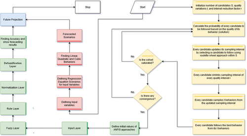
There are two main steps to forecasting future electricity consumption and scenario-independent factors (forecasting values of imports, exports, gross production, etc.) for energy scenarios, as seen in Figures 1 and 2. We proposed scenarios to predict independent factors such as imports, exports, gross generation, and transmitted energy for the first step. We used RES and independent factors, as shown in Figure 1. At the same time, CI was employed to obtain the optimum initial parameters (i.e., the number of rules, number of inputs, rate of initial learning, ratio of clustering, and number of epochs) to improve the performance of the ANFIS model. Then, CI-ANFIS was used to forecast electricity consumption by adopting scenario-independent factors to plan electricity consumption. After obtaining all forecast values, the framework was used to develop the energy scenarios.

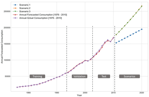
Figure 1. Dataset for forecasting electricity consumption.

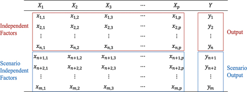
Figure 2. Application of the proposed forecasting framework where yellow, green, red, and blue stand for CI, ANFIS, RES, and future projections, respectively. note: RES has a line at the bottom, ANFIS has a line on the right, and CI has a line on top.

3.1. Regression equation scenarios

In the energy forecasting literature, scenario-independent factors are assumed to grow constantly. However, consistently growing values for scenario-independent factors do not reflect actual values. RES is offered here as a means of accurately forecasting scenario-independent factors. As seen in Figure 1, we can employ trend values to estimate unknown scenario values based on each factor. Then those values can be used to develop future scenarios. We considered three scenarios, linear, quadratic, and cubic, to represent the future trends of independent factors. We focused on the polynomial regression (i.e., linear, quadratic, and cubic relationships) because it is very clear that the points of the independent factors do not fit with linear regression. Based on the behaviours of independent factors, we defined the linear, quadratic, and cubic relationships, as seen in Figure 4. We did not use classical nonlinear regression because we used each independent factor as an input and output to predict its future values.

Scenario 1. The average growth rate of the independent factors was assumed to have a linear behaviour in the future, as seen in Equation (1)(1) $x_i={\beta }_0+{\beta }_1\times t$(1) .

(1) $x_i={\beta }_0+{\beta }_1\times t$(1)

where $x_i$ is $i$ th factor, ${\beta }_0$ and ${\beta }_1$ are regression coefficients, and $t$ is the past time lag.

Scenario 2. The average growth rate of the independent factors was assumed to have a quadratic behaviour, as seen in Equation (2)(2) $x_i={\beta }_0+{\beta }_1\times \hspace{0.17em}t+{\beta }_2\times t^2$(2) .

(2) $x_i={\beta }_0+{\beta }_1\times \hspace{0.17em}t+{\beta }_2\times t^2$(2)

Scenario 3. The average growth rate of the independent factors was assumed to have a cubic behaviour, as seen in Equation (3).

(3) $x_i={\beta }_0+{\beta }_1\times \hspace{0.17em}t+{\beta }_2\times t^2-{\beta }_3\times t^3$(3)

These equation-based scenarios were used to estimate the values of the scenario-independent factors, which demonstrated relationships with linear, quadratic, and cubic behaviours.

3.2. Adaptive neural fuzzy inference system approaches

ANFIS is not appropriate for systems based on traditional mathematical methods such as differential equations or poorly defined ones. The ANFIS structure consists of a Sugeno-type fuzzy approach that has the capacity for neural learning. This network is formed by combining nodes, which are placed in layers. The selection of membership functions in the fuzzy inference system (FIS) in ANFIS is arbitrary and varies by user. Additionally, the shape of the membership function depends on the number of parameters (Ediger & Kentel, 1999).

The FIS can be modelled without numerical analysis, using human information and an inference procedure employing if-then rules. Takagi and Sugeno (1985) first developed this type of fuzzy modelling. Since then, it has been used in many practical applications in the control, estimation, and inference fields (Moghadam et al., 2019).

3.2.1. General architecture

Assume a FIS where $x_1$ and $x_2$ are the independent factors, $y$ is the output, and the rule cluster for the first order Sugeno fuzzy model includes two “if-then-else” rules. The rules are shown in Equations (4)(4) $Rule1:If{x}_{1}is{A}_{1}and{x}_{2}is{B}_1,then{f}_1=p_1{x}_1+q_1{x}_2+r_1$(4) and (5(5) $Rule2:If{x}_{1}is{A}_{2}and{x}_{2}is{B}_2,then{f}_2=p_2{x}_1+q_2{x}_2+r_2$(5) ).

(4) $Rule1:If{x}_{1}is{A}_{1}and{x}_{2}is{B}_1,then{f}_1=p_1{x}_1+q_1{x}_2+r_1$(4)

(5) $Rule2:If{x}_{1}is{A}_{2}and{x}_{2}is{B}_2,then{f}_2=p_2{x}_1+q_2{x}_2+r_2$(5)

where $x_1$ and $x_2$ are the inputs, $p_1,p_2,q_1,q_2,r_1,$ and $r_2$ are the coefficients of the rule functions, and $A_1,A_2,B_1,$ and $B_2$ are predetermined constant values.

ANFIS arranges membership function parameters using the input-output dataset for the back-propagation algorithm in ANN, either alone or with least squares. In this way, the FIS is constituted. This arrangement allows the system to learn from the data that the fuzzy system models. It adapts according to the data modelled by itself.

3.2.2. ANFIS structure and work system

ANFIS is precisely constituted from six layers. This six-layer structure can be seen in Figure 3. The first layer is the input layer, where each node receives the input signal and transmits it to other layers. The output equation for each node is defined in Equations (6)(6) $O_1\left(i\right)=\mu A_i\left(x_1\right),i=1,2$(6) and (7(7) $O_2\left(i\right)=\mu B_i\left(x_2\right),i=1,2$(7) ).

(6) $O_1\left(i\right)=\mu A_i\left(x_1\right),i=1,2$(6)

(7) $O_2\left(i\right)=\mu B_i\left(x_2\right),i=1,2$(7)

Figure 3. Network structure for combination 4 with the: (a) CI-ANFIS GP model, (b) CI-ANFIS SC model, and (c) basic structure of ANFIS.

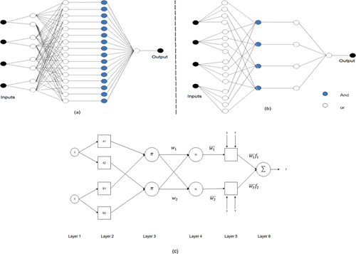
The second layer is the fuzzy layer, from which the memberships $\mu A_i\left(x_1\right)$ and $\mu B_i\left(x_2\right)$ are acquired. The activation function of the ANFIS model proposed in Jang (1993) was generalised as a membership function type and is used for cutting input values into fuzzy clusters. Every node acquired in this way is constituted from membership degrees bound to the membership functions and input values.

The third layer is the rule layer, where each node states the rules developed by the Sugeno inference system. The output of each node is the multiplication of membership degrees that comes from the second layer, as shown in Equation (8)(8) $y_i^3={\mathrm{\Pi }}_i=\mu A_i\left(x_1\right)\times \mu B_i\left(x_2\right)$(8) . The $y_i^3$ value in Equation (8)(8) $y_i^3={\mathrm{\Pi }}_i=\mu A_i\left(x_1\right)\times \mu B_i\left(x_2\right)$(8) shows the output value of Layer 3.

(8) $y_i^3={\mathrm{\Pi }}_i=\mu A_i\left(x_1\right)\times \mu B_i\left(x_2\right)$(8)

The fourth layer is the normalisation layer, where each node receives input from the nodes in the rule layer and estimates the normalisation of each rule. Equation (9)(9) $y_i^4=N_i=\frac{{\mu }_i}{{\sum }_{i=1}^n{\mu }_i}$(9) shows the calculation of the normalised priming level, ${\mu }_i$, as:

(9) $y_i^4=N_i=\frac{{\mu }_i}{{\sum }_{i=1}^n{\mu }_i}$(9)

where $n$ is the node number for this layer.

The fifth layer is the defuzzification layer. The goal is to calculate the weighted result value of each rule given at each node of the defuzzification layer. The output value of the node on the fifth layer is shown in Equation (10)(10) $y_i^5=y_i^4\left[p_i{x}_1+q_i{x}_2+r_i\right],i=1,2,\dots ,n$(10) .

(10) $y_i^5=y_i^4\left[p_i{x}_1+q_i{x}_2+r_i\right],i=1,2,\dots ,n$(10)

The $p_i,q_i,and{r}_i$ variables show the cluster of the resulting parameters for the $i$ _th rule.

The last layer is the multiplication layer, which consists of a node. This node is labeled $X$. In this layer, by summing the output values of each node in the fifth layer, the real output value of the ANFIS system is acquired. Finally, the calculation of $y$, which is the output value of the system, is carried out following Equation (11)(11) $y=\sum _{i=1}^n{y}_i^4\left[p_i{x}_1+q_i{x}_2+r_i\right]$(11) .

(11) $y=\sum _{i=1}^n{y}_i^4\left[p_i{x}_1+q_i{x}_2+r_i\right]$(11)

3.3. Cohort intelligence approach

Because the ANFIS system is complex, it is challenging to initialise with optimal parameters (Salleh & Hussain, 2016). ANFIS training includes structure learning and parameter optimisation. One challenge in ANFIS training is maintaining a balance between model complexity and accuracy (Azadeh, Ghaderi et al., 2008). ANFIS requires initial parameters; in the literature, these parameters are randomly initialised, resulting in unstable solutions. To overcome this issue, we propose using CI to optimise and initialise the ANFIS parameters.

CI is inspired by the nature and tendency of cohort individuals to learn from one another (Aladeemy et al. 2017). In this algorithm, every candidate supervises its behaviour (in a local search) and observes the behaviour of other candidates (in the global search) to identify the best behaviour. In this way, each candidate improves its overall behaviour until all candidates’ behaviours are similar, meaning cohort saturation is reached (Kulkarni et al., 2013). That is, no improvement can be attained in candidates’ behaviours.

As proposed by Kulkarni et al. (2013), the CI algorithm can be summarised as follows:

Consider the following minimisation problem:

(12) $subjectto{\mathrm{\Psi }}_{lower}^i\le {\alpha }_i\le {\mathrm{\Psi }}_{upper}^i,i=1,2,\dots ,n$(12)

The solution of the objective function $f\left(\alpha \right)$ is represented as the behaviour $i$ of an individual candidate $s$ in the cohort. The candidate is not the solution to the objective function; its change after attempting to learn is the solution. Every candidate tries to improve its behaviour by sampling behaviours $t$, which minimise $f\left(\alpha \right)$. Algorithm 1 shows the overall procedure for the CI-ANFIS approach.

Table

Algorithm 1: CI-ANFIS algorithm

Input: $S,Q,{\psi }_p\epsilon \left[{{\psi }_p}^{min},{{\psi }_p}^{max}\right],r\epsilon \left[0,1\right],L,\epsilon ,{\tau }^{max}$

Output: Best solution attained by the cohort Output: Forecast net electricity consumption

Procedure:

1: Set $\tau =1$

2: Generate random candidates, ${\mathrm{\Phi }}^S=\left\{{\varphi }^1,\dots ,{\varphi }^S\right\}$

3: Evaluate initial candidates, $F\left({\mathrm{\Phi }}^S\right)=\left\{f\left({\varphi }^1,\dots ,f\left({\varphi }^S\right)\right)\right\}$

4: for $l=1:L$ do

5: for $s=1:S$ do

6: Select a candidate’s behaviour to follow with a probability, $p^s$, using roulette selection approach, i.e., $p^s=\frac{f\left({\varphi }^s\right)}{{\sum }_{s=1}^{S}f\left({\varphi }^s\right)}$

7: Shrink sampling interval of each parameter ${\varphi }_p^s$ to its updated neighbourhood, ${\psi }_p^s\in \left[{\varphi }_p^s-\left(r\times \frac{\left|\left|{\psi }_p\right|\right|}{2}\right),{\varphi }_p^s+\left(r\times \frac{\left|\left|{\psi }_p\right|\right|}{2}\right)\right]$

8: Sample $Q$ qualities from the updated neighbourhood, ${\psi }_p^s$, for each parameter ${\varphi }_p^s$

9: Evaluate $Q$ sampled qualities and select the best behaviour to update the current behaviour of candidate $s$

10: end for

11: if $\left|\left(F{\left({\varphi }^s\right)}^l\right)-\left.\left(F{\left({\varphi }^s\right)}^{l-1}\right)\right|\right.\le \epsilon$ then

12: if $\left|\left(F{\left({\varphi }^s\right)}^l\right)-\left.\left(F{\left({\varphi }^s\right)}^{l-1}\right)\right|\right.\le \epsilon$ then

13: if $\left|\left(F{\left({\varphi }^s\right)}^l\right)-\left.\left(F{\left({\varphi }^s\right)}^{l-1}\right)\right|\right.\le \epsilon$ then

14: $\tau =\tau +1$

15: end if

16: end if

17: end if

18: if $\tau ={\tau }^{max}$ then

19: break

20: end if

21: end for 22: Best solution obtained by the cohort for vector of rules to be tested $Rt$, $n$= number of tests, $Ep$= number of epochs, and vector of Initial Learning Rates to be tested $TAt$,

29: for $i\in TAt$ do 30: for $j\in Rt$ do 31: for $l=1:n$ do 32: The input layer $O_1\left(i\right)=\mu A_i\left(x\right)$ and $O_2\left(i\right)=\mu B_i\left(x\right)$ 33: The fuzzy layer $y_i^3={\mathrm{\Pi }}_i=\mu A_i\left(x\right)\times \mu B_i\left(y\right)$ 34: The rule layer $y_i^4=N_i=\frac{{\mu }_i}{{\sum }_{i=1}^n{\mu }_i}$ 35: The normalisation layer $y_i^5=y_i^4\left[p_i{x}_1+q_i{x}_2+r_i\right]$ 36: The defuzzification layer $y=\sum _{i=1}^n{y}_i^4\left[p_i{x}_1+q_i{x}_2+r_i\right]$ end for 37: end for 38: end for 39: $Lowestvalidationerror=\mathrm{M}\mathrm{i}\mathrm{n}\mathrm{V},associatedFIS=\mathrm{C}\mathrm{h}\mathrm{e}\mathrm{c}\mathrm{k}\mathrm{F}\mathrm{i}\mathrm{s}$

For a cohort with several candidates S, every individual candidate $s=1,,2,\dots ,S$ has a set of behaviours ${\alpha }^s=\left({\alpha }_1^s,\dots ,{\alpha }_N^s\right)$ that create the total quality of its behaviour $f\left({\alpha }^s\right)$ (Xinqing et al., 1996).

Let $S=\left\{s=1,\dots ,S\right\}$ be the set of candidates in the cohort and ${\mathrm{\Phi }}^S=\left\{{\varphi }^1,\dots ,{\varphi }^S\right\}$ the set of behaviours of each candidate. In CI, each candidate uses roulette selection to identify and follow the other candidates’ behaviour. Given a sampling interval ${\mathrm{\Psi }}_p^s\in \left[{\mathrm{\Psi }}_p^{min,s},{\mathrm{\Psi }}_p^{max,s}\right]$, candidates then seek to improve their behaviour by sampling Q attributes for each parameter. This improvement can be considered to maximise $f\left({\varphi }^S\right)$

4. Application & results – forecasting net electricity consumption

4.1. Dataset description

We obtained monthly electricity consumption data between 1975 and 2010 from the Turkish Electricity Transmission Company (TEIAS), including independent factors and output values. We also collected the annual electricity consumption between 2011 and 2020 for comparing the forecasting values and actual values. Unlike previous studies that used annual observations, we collected monthly observations to facilitate a more accurate analysis. This dataset was collected and used by Tutun et al. (2015) to forecast volatile behaviour in net electricity consumption. The primary difference between this previous paper conducted by Tutun et al. (2015) and the current approach is that we use regression equation scenarios for forecasting demand along with ANFIS and Cohort intelligence approaches, which drastically improves the forecasting accuracy.

This dataset included 10 independent factors (as date (monthly), gross income, population, load (hourly), immediate load, imports, exports, gross production, transmitted energy, net electricity consumption, electricity consumption, and loss of electricity) and 420 observations. Among the 420 observations, 210 were used as a training set, 105 as a validation set, and 105 as a test set. Following earlier work on forecasting electricity consumption in Turkey (Sözen & Arcaklioglu, 2007; Toksari, 2009), we used four independent factors (i.e., transmitted energy, gross production, imports, and exports) to predict net electricity consumption.

In this study, we defined four combinations based on the independent factors and output values (see, Table 2). The best model was derived by quantifying each method’s performance. Then, the projections were determined for scenarios using linear, quadratic, and cubic equations.

Table 2. Combination of independent factors where the output variable is net electricity consumption.

Combination(s)	Independent Factor(s)
Combination 1	Transmitted energy
Combination 2	Transmitted energy and gross production
Combination 3	Transmitted energy, gross production, and exports
Combination 4	Transmitted energy, gross production, exports, and imports

4.2. Performance measures

For performance measures, we investigated the difference between the estimated and actual values of net electricity consumption, employing three error metrics: the Mean Absolute Percent Error (MAPE), root mean square error (RMSE), and R squared ($R^2$). MAPE in Equation (13)(13) $MAPE=\frac{\left({\sum }_{i=1}^n\left|\frac{Y_i-F_i}{Y}\right|\right)}{n}\ast 100$(13) is a means of calculating the fitted values for forecasting. Results can be calculated as percentages.

(13) $MAPE=\frac{\left({\sum }_{i=1}^n\left|\frac{Y_i-F_i}{Y}\right|\right)}{n}\ast 100$(13)

where $F_i$ is the estimated net electricity consumption for observation $i$ and $Y_i$ is the actual net electricity consumption for observation $i$. RMSE in Equation (14)(14) $RMSE=\hspace{0.17em}\sqrt{\frac{\left({\sum }_{i=1}^n{(Y_i-F_i)}^2\right.}{n}}$(14) determines the sample standard deviation of difference between the estimated and actual values.

(14) $RMSE=\hspace{0.17em}\sqrt{\frac{\left({\sum }_{i=1}^n{(Y_i-F_i)}^2\right.}{n}}$(14)

$R^2$ in Equation (15)(15) $R^2=1-\hspace{0.17em}\frac{{\sum }_{i=1}^n{(Y_i-F_i)}^2}{{\sum }_{i=1}^n{(Y_i-{\mu }_i)}^2}$(15) is the square of the correlation coefficient for checking the goodness of fit of the observations.

(15) $R^2=1-\hspace{0.17em}\frac{{\sum }_{i=1}^n{(Y_i-F_i)}^2}{{\sum }_{i=1}^n{(Y_i-{\mu }_i)}^2}$(15)

where $\mu$ is the mean of actual net electricity consumption.

4.3. Regression equation scenarios

This section describes the model summary and parameter estimates to determine the correct coefficients for the equations. The scenarios are as follows.

Scenario 1. It is accepted that the average growth rate of the independent factors of gross production ($x_1$), electricity imports ($x_2$), transmitted electricity ($x_3$), and electricity exports ($x_4$) will have a linear behaviour in the future (using past lags ($t$)), as seen in Equations (16)(16) $x_1=-1182.274+40.348\times t_1$(16) to (19).

(16) $x_1=-1182.274+40.348\times t_1$(16)

(17) $x_2=34.538+0.667\times t_2$(17)

(18) $x_3=-946.180+33.591\times t_3$(18)

(19) $x_4=-33.195+0.371\times t_4$(19)

Scenario 2. It is accepted that the average growth rate of the independent factors will have a quadratic behaviour in the future, as seen in Equations (20)(20) ${ }_1=1258.198+5.65\times t_1+0.082\times t_1^2$(20) to (23).

(20) ${ }_1=1258.198+5.65\times t_1+0.082\times t_1^2$(20)

(21) $x_2=41.517+0.18\times t_2+0.006\times t_2^2$(21)

(22) $x_3=1285.642+1.859\times t_3+0.075\times t_3^2$(22)

(23) $x_4=8.606-0.223\times t_4+0.001\times t_4^2$(23)

Scenario 3. It is accepted that the average growth rate of the independent factors will have a cubic behaviour in the future, as seen in Equations (24)(24) $x_1=1388.340+1.962\times t_1+0.104\times t_1^2-0.00003463\times t_1^3$(24) to (27).

(24) $x_1=1388.340+1.962\times t_1+0.104\times t_1^2-0.00003463\times t_1^3$(24)

(25) $x_2=23.206+2.691\times t_2-0.068\times t_2^2+0.001\times t_2^3$(25)

(26) $x_3=942.013+11.596\times t_3+0.18\times t_3^2+0.00009145\times t_3^3$(26)

(27) $x_4=-8.072+0.249\times t_4-0.001\times t_4^2+0.000004438\times t_4^3$(27)

In the equations, we have electricity import ($x_2$), transmitted electricity ($x_3$), and electricity export ($x_4$) values.

These equation-based scenarios are used to estimate the values of scenario-independent factors, which have either quadratic, cubic, or linear behaviour. From Figure 4, one can see that linear behaviour did not capture the trend in independent factors. As a result of the independent factors seen in Tables 3, 4, 5 and 6, it was determined that the equation-based scenarios were appropriate for forecasting because they were significant and fit all behaviours in Figure 4.

Table 3. Model summary and parameter estimates for gross production $\left(x_1\right).$.

	Model Summary			Parameter Estimates
Equation	$R^2$ value	$F$ Measure	$p$-value	${\beta }_0$	${\beta }_1$	${\beta }_2$	${\beta }_3$
Linear	0.969	6,473.606	0	−1,182.274	40.348
Quadratic	0.993	14,111.205	0figure	1,258.198	5.650	0.082
Cubit	0.993	9,445.665	0	1,388.340	1.962	0.104	−0.00003

Figure 4. Fitting of independent factors with three equations.

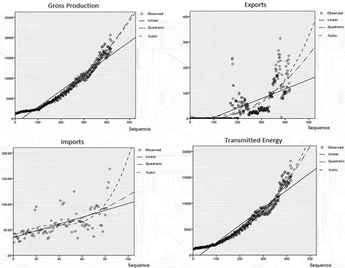
Table 4. Model summary and parameter estimates for electricity energy imports $\left(x_2\right)$.

	Model Summary			Parameter Estimates
Equation	$R^2$ value	$F$ Measure	$p$-value	${\beta }_0$	${\beta }_1$	${\beta }_2$	${\beta }_3$
Linear	0.609	48.311	0	34.538	0.667
Quadratic	0.619	25.203	0	41.517	0.18	0.006
Cubit	0.665	21.163	0	23.206	2.691	−0.068	0.001

Table 5. Model summary and parameter estimates for transmitted electricity $\left(x_3\right)$.

	Model Summary			Parameter Estimates
Equation	$R^2$ value	$F$ Measure	$p$-value	${\beta }_0$	${\beta }_1$	${\beta }_2$	${\beta }_3$
Linear	0.96	4915.186	0	−946.180	33.591
Quadratic	0.988	8548.660	0	1285.642	1.859	0.075
Cubit	0.988	5917.123	0	942.013	11.596	0.018	0.00009

The independent factors were calculated for the years 2011 to 2020 using RES. Then, the scenario-independent factors were used to forecast the net electricity consumption during future years and months via the best model. The values of the independent factors in future years (i.e., 2011 to 2020) were determined according to the trends in independent factors for the years 1976 to 2010, by scenario. Estimations of the scenarios were made for future years and months via a mathematical formula established using the best model.

4.4. Process of obtaining the best model

CI algorithms work better than do other heuristic algorithms (Azadeh, Ghaderi et al., 2008; Sangrody & Zhou, 2016). We used CI to optimise the SC and GP parameters of ANFIS. The methods were used separately, their results compared, and the best model determined (as seen in Figure 5). We used RES in the framework because we needed to forecast the future values of each independent factor between 2010 and 2020. Then, we used our best model (CI-ANFIS) with the forecasted independent factors. Therefore, we presented our forecasted net electricity consumption between 2010 and 2020.

Figure 5. Framework for forecasting net electricity consumption.

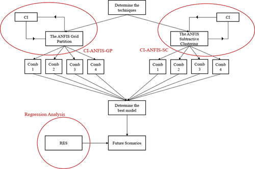
Figure 5. Scatterplot of the test set for combination 3.

4.4.1. Formation of the CI-ANFIS grid partition model

This method constitutes a rule using training, validation, and test sets. The GP method differs from others in terms of rule formation. In this method, the rules for each of the input membership functions in the second layer of the system are set. The method takes its name from this characteristic. This is shown in detail in the model’s structure, which is constituted from four inputs and one output via GP (Combination 4), as seen in Figures 3 and 5. The user determines the type of output membership function given at the fourth layer (see, Figure 3). In the present study, the output membership functions were determined to be constant and linear, and the epoch numbers for the best model were 10 and 100.

Finally, the CI-ANFIS was trained using the rules formed with the training data, according to the GP method. If the CI-ANFIS parameters reached optimum results at the end of the training, they were applied at the test level, and the estimating procedure was carried out. If it was not possible to obtain the optimum results, the CI-ANFIS was retrained.

4.4.2. Formation of the CI-ANFIS subtractive clustering model

The flow scheme of the SC method is logically the same as that of GP. The training, validation, and test sets are used to compose the rules of the CI-ANFIS model. When setting the rules for the second layer, the number and types of membership functions (i.e., Gaussian (GaussMF) or Triangular (TriMF)) are adjusted according to the second layer’s input and output data relationships. Instead of examining all rules (as in GP), output membership functions are determined by setting only the necessary rules. This model is shown in layer form in Figure 3. The structure and practicability of the models increase according to the status of the data used in the learning process. The data were distributed non-linearly and periods of economic crisis (such as in 2001) prevented setting a rule properly. As only necessary rules are used instead of all rules, the SC method offered better results.

The results were compared to determine the model with the lowest error values. As shown in Figure 6, combinations according to independent factors were determined from the model formed from four independent factors and one output. The combinations for each method are shown in Table 7.

Table 6. Model summary and parameter estimates for electricity export $\left(x_4\right)$.

	Model Summary			Parameter Estimates
Equation	$R^2$ value	$F$ Measure	$p$-value	${\beta }_0$	${\beta }_1$	${\beta }_2$	${\beta }_3$
Linear	0.718	444.839	0	−33.195	0.371
Quadratic	0.778	317.21	0	8.606	−0.223	0.001
Cubit	0.783	219.799	0	−8.072	0.249	−0.001	0.000004

Table 7. Lowest error values for the CI-ANFIS approach.

	Error for Testing Level			Error for Validation Level
Type of Error	RMSE	MAPE	$R^2$	RMSE	MAPE	$R^2$
Combination 1	134.3267	1.8660	0.9975	172.8556	1.1883	0.9962
Combination 2	230.9704	2.9297	0.9987	138.7800	0.9650	0.9955
Combination 3	107.8149	1.4917	0.9973	219.4464	1.5945	0.9939
Combination 4	81.8181	1.1627	0.9985	505.1039	3.9509	0.9935

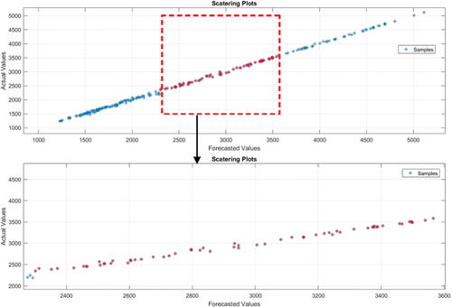
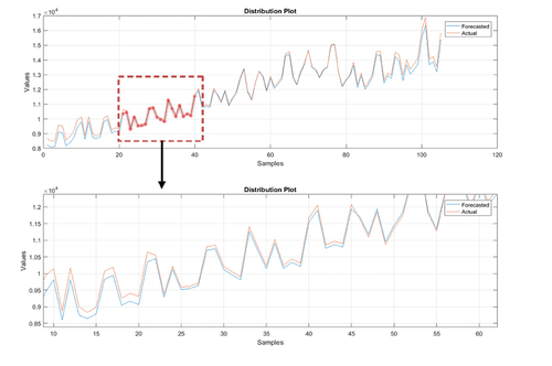
Figure 6. Distribution plot of the test set for combination 3.

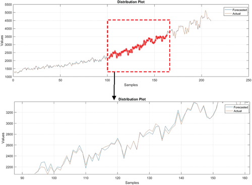
Figure 7. Scatterplot of the validation set for combination 3.

From Table 7, it can be seen that the lowest MAPE error value was obtained by Combination 3 (for both the validation and test sets). The best combination model among the models developed with the CI-ANFIS method was Combination 3, as shown in Table 8.

Table 8. Best CI-ANFIS model for combination 3.

	Testing Level	Validation Level
$R^2$	0.9973	0.9939
RMSE	107.8149	219.4464
MAPE	1.4917	1.5945

As shown in Tables 6 to 8, Combination 3 was the best model, with $R^2=0.9973$, $RMSE=107.8149$, and $MAPE=1.49$. As for the initial parameters obtained using CI, we found 0.59 for the coefficient value of SC and 21 for the epoch number. The actual and forecasted values of the test set are illustrated in the scatterplots in Figures 5 to 8. From those figures, one can see that the forecasted values were very close to actual values.

Figure 8. Distribution plot for the validation set for combination 3.

5. Discussion

According to the above results, the method was applied to forecast future net electricity consumption using a real dataset obtained from Turkey, as seen in Figure 9.

Figure 9. Annual forecasting values obtained using the best model structure.

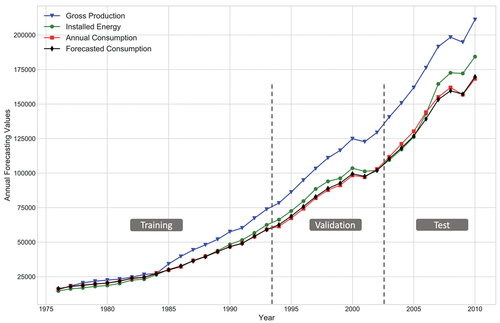
Our framework forecasted electricity consumption with a 1.49% error rate, while the Turkish government forecasted at an error rate of 13.86% (see, Table 9). The estimates were made for the years 2011 to 2020, with the model constituting three scenarios. The estimates for future years and months were made using Combination 3 (see, Table 8) and the CI-ANFIS SC process for each scenario. To determine future monthly independent factors, estimates were formed using RES. The best model was applied to three scenarios: linear, quadratic, and cubic regression. Previous studies used future values of independent factors that grew at a constant rate (Ediger & Tatlidil, 2002; Erdogdu, 2007; Hamzaçebi, 2007). However, this method fails to accurately reflect the values of future independent factors because the increase in estimated inputs is considered to be linear. Hence, to obtain a more accurate estimation of the actual independent factors, these three equations (i.e., RES) incorporated trend values. We used the model summaries and parameter estimates for four independent factors, as seen in Tables 3 to 6.

Table 9. Comparison of the proposed framework results with other representative studies. note: MAED: model for analysis of energy demand.

	2008			2009
Researchers	Forecasted Value	Actual Value	MAPE Error	Forecasted Value	Actual Value	MAPE Error
MAED Simulation	168.60	161.95	4.1%	184.40	156.89	13.86%
Hamzacebi	173.59	161.95	7.2%	189.47	156.89	16.99%
Erdogdu	146.37	161.95	9.6%	145.14	156.89	10.4%
Tutun	159.643	161.95	1.47%	157.168	156.89	0.283%
Kavaklioglu	165.94	161.95	2.46%	175.04	156.89	11.5%
Proposed Approach	159.655	161.95	1.417%	157.195	156.89	0.19%

Figure 12 shows the forecasted net electricity consumption for Turkey between 2011 and 2020, using the three scenarios. These values can be employed for both planning and scheduling. The input values in future years (2011–2020) were determined according to the growth rates of input values from 1975 to 2010. Future inputs were estimated for future years via the mathematical formula established by the best model. As seen in Figure 10, we forecasted the future annual gross production using linear, quadratic, and cubic behaviours. The linear behaviour did not represent the trend because it decreased after 2010 when it should have increased. This meant that future gross production would have either a cubic or quadratic behaviour. We also forecasted the future annual installed energy using the three scenarios (see, Figure 11), which also indicated the need to use nonlinear behaviour (either cubic or quadratic) for this input. Finally, as shown in Figure 12, by using the forecasted annual gross production and installed energy as inputs, we were able to use the best model (i.e., CI-ANFIS SC) to forecast the future annual electricity consumption. Interestingly, the best model and either quadratic or cubic behaviour produced almost the same results and were very close to the real-world values.

Figure 10. Annual gross production for scenarios 1 through 3.

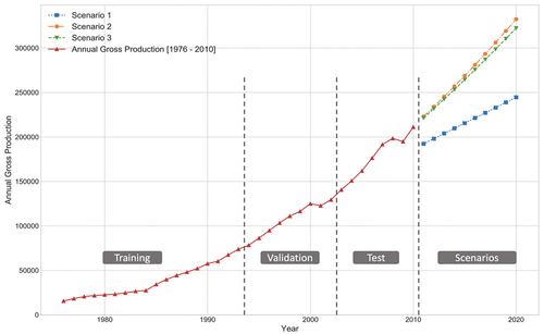
Figure 11. Annual installed energy values for scenarios 1 through 3.

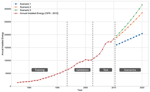
Figure 12. Annual forecasted consumption values for scenarios 1 through 3.

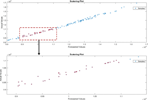
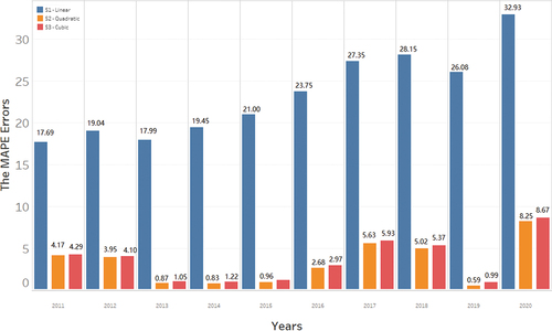
We then compared our forecasts with studies in the literature that predicted net electricity consumption. Our predicted results were within 1.49% of actual consumption, and our estimates were closer to actual use than were other estimates found in the literature. As shown in Table 9, in this study, the simulation indicated that results obtained were better than the predictions made by the Model for Analysis of Energy Demand (MAED) simulation tool used by the Minister of Energy and Natural Sources (MENR; Erdogdu, 2007; Hamzaçebi, 2007; Kavaklioglu, 2011; Tutun et al., 2015). As seen in Table 9, the differences between the estimated and actual values were very small. For 2008 and 2009, the model predicted 159.64 TW in 2008 and 157.17 TW in 2009, whereas the actual values were 161.95 TW in 2008 and 156.89 TW in 2009. These values correspond to MAPEs of 1.417% in 2008 and 0.19% in 2009. Moreover, based on the ten-year scenario, we compared our forecasted net electricity consumption between 2011 and 2020 with actual electricity consumption, as seen in Figure 13. Our framework predicted net electricity consumption with the ten-year average error rates of 3.29% and 3.56% for the quadratic and cubic scenarios’ independent factors, respectively. Additionally, we showed that we could not use the linear scenario’s independent factors because that scenario resulted in around a ten-year average MAPE rate of 23%. This analysis proves that policymakers need to follow nonlinear-based scenarios with the best model.

Figure 13. Comparison results for the years 2011–2020. note: the errors are calculated as percentage.

Again, compared with other studies, the best model achieved better results for both years when the monthly data were considered, and regression equations were employed to forecast future inputs (rather than using a constant growth rate). As shown in Table 9 and Figure 12, contrary to other studies that used constant mean values for future inputs, it was better to use regression equations as scenarios for independent factor forecasting. These produced more estimates of the net electricity consumption for Turkey from 2011 to 2020. These scenarios were evaluated using equations with trends that affected the independent factors. The best model was used to forecast the future net electricity demand.

6. Conclusion

Forecasting net electricity consumption is essential for adequately managing, controlling, operating, and marketing a power system. However, medium-term and long-term forecasting covering months to years is more challenging than forecasting in the short term because of the uncertainty of independent predictors on lengthy forecasting horizons. This study proposes a forecasting model and applies it to a real dataset obtained from Turkey to predict monthly and yearly net electricity consumption. In this model, economic, population, and historical data of net consumption were applied as inputs. In addition, gross production, electricity import, transmitted energy, and electricity export data were applied in the forecasting model as independent factors for net electricity consumption. Eight models were formed, and the best model structure was determined using the CI-ANFIS sub-clustering and CI-ANFIS GP for each combination, comparing the error metrics of the testing and validation sets. A new RES approach was also developed to forecast independent predictors’ values when establishing future scenarios for forecasting net electricity consumption values.

In this research, future projections were made and discussed according to three scenarios, providing helpful information for policymakers. We showed that we could use independent predictors to forecast future electricity consumption with a high level of accuracy. Moreover, our framework can be extended by considering advanced scenario forecasting approaches. Therefore, future work will develop nonlinear scenario forecasting approaches.

Finally, comparing the results with other studies indicated the proposed method’s efficacy in forecasting error metrics for the proposed forecasting model. The error rates were much lower than those of other studies for monthly and annual net energy consumption. Thus, the forecasting methodology and results provide an efficient tool for policymakers and power system managers to use when planning and scheduling energy.

The business implications of this study are numerous. First, energy companies can utilise this proposed framework to better estimate the demand, allowing them to better plan and use their resources. Second, using this framework, energy companies can minimise waste as energy is difficult to store if there is a surplus. Third, energy generators and suppliers selling electricity to customers can use the energy demand predictions as input to determine customised pricing strategies. In addition to these implications related to private energy companies, there are other implications pertinent to the government sector. For example, legislators and policymakers can use the assessments and forecasts obtained from our framework to develop energy policies that aim to conserve resources and protect the environment. Furthermore, relevant government agencies can ensure energy reliability, enhance the country’s economy, and protect public health and safety using the predictions obtained from this framework.

This study is not without any limitations. For instance, our data collection process was guided by the previous literature. Thus, we have not considered weather patterns and seasonal variations. Additionally, the dataset used in this study includes observations since 1975; thus, it was difficult to obtain reliable factors/variables regarding global warming and weather patterns. These additional variables can be incorporated in our future studies. Additionally, our dataset contained monthly electricity consumption. Future studies can attempt to collect weekly or daily electricity consumption data to improve the forecasting error rates.

Acknowledgments

This research did not receive any specific grant from funding agencies in the public, commercial, or not-for-profit sectors.

Disclosure statement

No potential conflict of interest was reported by the author(s).

References

- Aladeemy, M., Tutun, S., & Khasawneh, M. T. (2017). A new hybrid approach for feature selection and support vector machine model selection based on self-adaptive cohort intelligence. Expert Systems with Applications, 88, 118–131. https://doi.org/10.1016/j.eswa.2017.06.030
- Ardakani, F. J., & Ardehali, M. M. (2014). Long-term electrical energy consumption forecasting for developing and developed economies based on different optimized models and historical data types. Energy, 65(1), 452–461. https://doi.org/10.1016/j.energy.2013.12.031
- Arora, S., & Taylor, J. W. (2018). Rule-based autoregressive moving average models for forecasting load on special days: A case study for France. European Journal of Operational Research, 266(1), 259–268. https://doi.org/10.1016/j.ejor.2017.08.056
- Ayvaz, B., & Kusakci, A. O. (2017). Electricity consumption forecasting for Turkey with nonhomogeneous discrete grey model. Energy Sources, Part B: Economics, Planning, and Policy, 12(3), 260–267. https://doi.org/10.1080/15567249.2015.1089337
- Azadeh, A., Ghaderi, S. F., & Sohrabkhani, S. (2008). Annual electricity consumption forecasting by neural network in high energy consuming industrial sectors. Energy Conversion and Management, 49(8), 2272–2278. https://doi.org/10.1016/j.enconman.2008.01.035
- Azadeh, A., Saberi, M., Ghaderi, S. F., Gitiforouz, A., & Ebrahimipour, V. (2008). Improved estimation of electricity demand function by integration of fuzzy system and data mining approach. Energy Conversion and Management, 49(8), 2165–2177. https://doi.org/10.1016/j.enconman.2008.02.021
- Azadeh, A., Saberi, M., Gitiforouz, A., & Saberi, Z. (2009). A hybrid simulation-adaptive network based fuzzy inference system for improvement of electricity consumption estimation. Expert Systems with Applications, 36(8), 11108–11117. https://doi.org/10.1016/j.eswa.2009.02.081
- Azadeh, A., Taghipour, M., Asadzadeh, S. M., & Abdollahi, M. (2014). Artificial immune simulation for improved forecasting of electricity consumption with random variations. International Journal of Electrical Power and Energy Systems, 55(1), 205–224. https://doi.org/10.1016/j.ijepes.2013.08.017
- Bessec, M., & Fouquau, J. (2018). Short-run electricity load forecasting with combinations of stationary wavelet transforms. European Journal of Operational Research, 264(1), 149–164. https://doi.org/10.1016/j.ejor.2017.05.037
- Catalão, J. P. S., Pousinho, H. M. I., & Mendes, V. M. F. (2011). Hybrid wavelet-PSO-ANFIS approach for short-term electricity prices forecasting. IEEE Transactions on Power Systems, 26(1), 137–144. https://doi.org/10.1109/TPWRS.2010.2049385
- Crider, J. (2020). COVID-19 Bankrupts 19 energy (oil & gas) companies. CleanTechnica.https://cleantechnica.com/2020/08/05/covid-19-bankrupts-19-energy-oil-gas-companies. April/April/2021
- Duan, J., Qiu, X., Ma, W., Tian, X., & Shang, D. (2018). Electricity consumption forecasting scheme via improved LSSVM with maximum correntropy criterion. Entropy, 20(2), 112. https://doi.org/10.3390/e20020112
- Duran Toksari, M. (2007). Ant colony optimization approach to estimate energy demand of Turkey. Energy Policy, 35(8), 3984–3990. https://doi.org/10.1016/j.enpol.2007.01.028
- Ediger, V. Ş., & Akar, S. (2007). ARIMA forecasting of primary energy demand by fuel in Turkey. Energy Policy, 35(3), 1701–1708. https://doi.org/10.1016/j.enpol.2006.05.009
- Ediger, V. Ş., & Kentel, E. (1999). Renewable energy potential as an alternative to fossil fuels in Turkey. Energy Conversion and Management, 40(7), 743–755. https://doi.org/10.1016/S0196-8904(98)00122-8
- Ediger, V. Ş., & Tatlidil, H. (2002). Forecasting the primary energy demand in Turkey and analysis of cyclic patterns. Energy Conversion and Management, 43(4), 473–487. https://doi.org/10.1016/S0196-8904(01)00033-4
- Erdogdu, E. (2007). Electricity demand analysis using cointegration and ARIMA modelling: A case study of Turkey. Energy Policy, 35(2), 1129–1146. https://doi.org/10.1016/j.enpol.2006.02.013
- Hamzaçebi, C. (2007). Forecasting of Turkey’s net electricity energy consumption on sectoral bases. Energy Policy, 35(3), 2009–2016. https://doi.org/10.1016/j.enpol.2006.03.014
- Hong, T., & Fan, S. (2016). Probabilistic electric load forecasting: A tutorial review. International Journal of Forecasting, 32(3), 914–938. https://doi.org/10.1016/j.ijforecast.2015.11.011
- Hu, Y. C. (2017). Electricity consumption prediction using a neural-network-based grey forecasting approach. Journal of the Operational Research Society, 68(10), 1259–1264. https://doi.org/10.1057/s41274-016-0150-y
- IEA. (2020). COVID-19 impact on electricity. https://www.iea.org/reports/covid-19-impact-on-electricity, April/28/2021
- (IEA). Global Energy Review. (2020). The impacts of the Covid-19 crisis on global energy demand and CO2 emissions. https://www.iea.org/reports/global-energy-review-2020. April/28/2021
- Jang, J. S. R. (1993). ANFIS: adaptive-network-based fuzzy inference system. IEEE Transactions on Systems, Man, and Cybernetics, 23(3), 665–685. https://doi.org/10.1109/21.256541
- Kaboli, S. H. A., Fallahpour, A., Selvaraj, J., & Rahim, N. A. (2017). Long-term electrical energy consumption formulating and forecasting via optimized gene expression programming. Energy, 126(1), 144–164. https://doi.org/10.1016/j.energy.2017.03.009
- Kankal, M., & Uzlu, E. (2017). Neural network approach with teaching–learning-based optimization for modeling and forecasting long-term electric energy demand in Turkey. Neural Computing & Applications, 28(1), 737–747. https://doi.org/10.1007/s00521-016-2409-2
- Kavaklioglu, K. (2011). Modeling and prediction of Turkey’s electricity consumption using support vector regression. Applied Energy, 88(1), 368–375. https://doi.org/10.1016/j.apenergy.2010.07.021
- Kavaklioglu, K. (2014). Robust electricity consumption modeling of Turkey using singular value decomposition. International Journal of Electrical Power and Energy Systems, 54(1), 268–276. https://doi.org/10.1016/j.ijepes.2013.07.020
- Kaytez, F. (2020). A hybrid approach based on autoregressive integrated moving average and least-square support vector machine for long-term forecasting of net electricity consumption. Energy, 197(1), 117200. https://doi.org/10.1016/j.energy.2020.117200
- Kaytez, F., Taplamacioglu, M. C., Cam, E., & Hardalac, F. (2015). Forecasting electricity consumption: A comparison of regression analysis, neural networks and least squares support vector machines. International Journal of Electrical Power and Energy Systems, 67(1), 431–438. https://doi.org/10.1016/j.ijepes.2014.12.036
- Kermanshahi, B., & Iwamiya, H. (2002). Up to year 2020 load forecasting using neural nets. International Journal of Electrical Power and Energy Systems, 24(9), 789–797. https://doi.org/10.1016/S0142-0615(01)00086-2
- Kheirkhah, A., Azadeh, A., Saberi, M., Azaron, A., & Shakouri, H. (2013). Improved estimation of electricity demand function by using of artificial neural network, principal component analysis and data envelopment analysis. Computers & Industrial Engineering, 64(1), 425–441. https://doi.org/10.1016/j.cie.2012.09.017
- Kulkarni, A. J., Baki, M. F., & Chaouch, B. A. (2016). Application of the cohort-intelligence optimization method to three selected combinatorial optimization problems. European Journal of Operational Research, 250(2), 427–447. https://doi.org/10.1016/j.ejor.2015.10.008
- Kulkarni, A. J., Durugkar, I. P., & Kumar, M. (2013). Cohort intelligence: A self supervised learning behavior. Proceedings - 2013 IEEE international conference on systems, man, and cybernetics, SMC 2013, 1396–1400.
- Lee, Y. S., & Tong, L. I. (2011). Forecasting energy consumption using a grey model improved by incorporating genetic programming. Energy Conversion and Management, 52(1), 147–152. https://doi.org/10.1016/j.enconman.2010.06.053
- Marcjasz, G., Uniejewski, B., & Weron, R. (2019). On the importance of the long-term seasonal component in day-ahead electricity price forecasting with NARX neural networks. International Journal of Forecasting, 35(4), 1520–1532. https://doi.org/10.1016/j.ijforecast.2017.11.009
- Marcjasz, G., Uniejewski, B., & Weron, R. (2020). Probabilistic electricity price forecasting with NARX networks: Combine point or probabilistic forecasts? International Journal of Forecasting, 36(2), 466–479. https://doi.org/10.1016/j.ijforecast.2019.07.002
- Moghadam, R. G., Izadbakhsh, M. A., Yosefvand, F., & Shabanlou, S. (2019). Optimization of ANFIS network using firefly algorithm for simulating discharge coefficient of side orifices. Applied Water Science, 9(4), 1–12. https://doi.org/10.1007/s13201-019-0950-8
- Moret, S., Babonneau, F., Bierlaire, M., & Maréchal, F. (2020). Decision support for strategic energy planning: A robust optimization framework. European Journal of Operational Research, 280(2), 539–554. https://doi.org/10.1016/j.ejor.2019.06.015
- Oğcu, G., Demirel, O. F., & Zaim, S. (2012). Forecasting electricity consumption with neural networks and support vector regression. Procedia-Social and Behavioral Sciences, 58 1, 1576–1585.
- Ozturk, H. K., Ceylan, H., Canyurt, O. E., & Hepbasli, A. (2005). Electricity estimation using genetic algorithm approach: A case study of Turkey. Energy, 30(7), 1003–1012. https://doi.org/10.1016/j.energy.2004.08.008
- Pousinho, H. M. I., Mendes, V. M. F., & Catalão, J. P. S. (2011). A hybrid pso-anfis approach for short-term wind power prediction in Portugal. Energy Conversion and Management, 52(1), 397–402. https://doi.org/10.1016/j.enconman.2010.07.015
- Pousinho, H. M. I., Mendes, V. M. F., & Catalão, J. P. S. (2012). Short-term electricity prices forecasting in a competitive market by a hybrid PSO-ANFIS approach. International Journal of Electrical Power and Energy Systems, 39(1), 29–35. https://doi.org/10.1016/j.ijepes.2012.01.001
- Salleh, M. N. M., & Hussain, K. (2016). A review of training methods of ANFIS for applications in business and economics. International Journal of U- and E- Service, Science and Technology, 9(7), 165–172. https://doi.org/10.14257/ijunesst.2016.9.7.17
- Sangrody, H., & Zhou, N. (2016). An initial study on load forecasting considering economic factors. IEEE power and energy society general meeting, 2016–November.
- Sangrody, H., Zhou, N., Tutun, S., Khorramdel, B., Motalleb, M., & Sarailoo, M. (2018). Long term forecasting using artificial intelligence methods. In 2018 IEEE power and energy conference at Illinois (PECI) (pp. 1–5). IEEE. https://doi.org/10.1109/peci.2018.8334980
- Simsek, S., Genc, O., Albizri, A., Dinc, S., & Gonen, B. (2020a). Artificial neural network incorporated decision support tool for point velocity prediction. Journal of Business Analytics, 3(1), 67–78. https://doi.org/10.1080/2573234X.2020.1751569
- Simsek, S., Gumus, M., Khalafalla, M., & Issa, T. B. (2020b). A hybrid data analytics approach for high-performance concrete compressive strength prediction. Journal of Business Analytics, 3(2), 158–168. https://doi.org/10.1080/2573234X.2020.1760741
- Sözen, A. (2009). Future projection of the energy dependency of Turkey using artificial neural network. Energy Policy, 37(11), 4827–4833. https://doi.org/10.1016/j.enpol.2009.06.040
- Sözen, A., & Arcaklioglu, E. (2007). Prediction of net energy consumption based on economic indicators (GNP and GDP) in Turkey. Energy Policy, 35(10), 4981–4992. https://doi.org/10.1016/j.enpol.2007.04.029
- Steinbuks, J. (2019). Assessing the accuracy of electricity production forecasts in developing countries. International Journal of Forecasting, 35(3), 1175–1185. https://doi.org/10.1016/j.ijforecast.2019.04.009
- Takagi, T., & Sugeno, M. Fuzzy identification of systems and its applications to modeling and control. (1985). IEEE Transactions on Systems, Man, and Cybernetics, 15(1), 116–132. SMC-. https://doi.org/10.1109/TSMC.1985.6313399
- Toksari, M. D. (2009). Estimating the net electricity energy generation and demand using the ant colony optimization approach: case of Turkey. Energy Policy, 37(3), 1181–1187. https://doi.org/10.1016/j.enpol.2008.11.017
- Toksari, M. D. (2016). A hybrid algorithm of ant colony optimization (ACO) and Iterated Local Search (ILS) for estimating electricity domestic consumption: case of Turkey. International Journal of Electrical Power and Energy Systems, 78(1), 776–782. https://doi.org/10.1016/j.ijepes.2015.12.032
- Tunç, M., Çamdali, Ü., & ParmaksizogluC.2006. Comparison of Turkey’s electrical energy consumption and production with some European countries and optimization of future electrical power supply investments in Turkey. Energy Policy, [ Turkey | World Energy Council. July 6, 2020, from], 34(1), 50–59. https://www.worldenergy.org/impact-communities/members/entry/turkey
- Tutun, S., Chou, C. A., & Caniyilmaz, E. (2015). A new forecasting framework for volatile behavior in net electricity consumption: A case study in Turkey. Energy, 93(1), 2406–2422. https://doi.org/10.1016/j.energy.2015.10.064
- Ünler, A. (2008). Improvement of energy demand forecasts using swarm intelligence: the case of Turkey with projections to 2025. Energy Policy, 36(6), 1937–1944. https://doi.org/10.1016/j.enpol.2008.02.018
- Xinqing, L., Tsoukalas, L. H., & Uhrig, R. E. (1996). Neurofuzzy approach for the anticipatory control of complex systems. IEEE international conference on fuzzy systems, 1, 587–593.
- Ziel, F., & Liu, B. (2016). Lasso estimation for GEFCom2014 probabilistic electric load forecasting. International Journal of Forecasting, 32(3), 1029–1037. https://doi.org/10.1016/j.ijforecast.2016.01.001