Subdiffusive fractional Black–Scholes model for pricing currency options under transaction costs

Abstract

A new framework for pricing European currency option is developed in the case where the spot exchange rate follows a subdiffusive fractional Black–Scholes. An analytic formula for pricing European currency call option is proposed by a mean self-financing delta-hedging argument in a discrete time setting. The minimal price of a currency option under transaction costs is obtained as time-step $\mathrm{\Delta }t={\left(\frac{t^{\alpha -1}}{\mathrm{\Gamma }(\alpha )}\right)}^{-1}{\left(\frac{2}{\pi }\right)}^{\frac{1}{2H}}{\left(\frac{k}{\sigma }\right)}^{\frac{1}{H}}$, which can be used as the actual price of an option. In addition, we also show that time-step and long-range dependence have a significant impact on option pricing.

Keywords:

• subdiffusion process
• currency option
• transaction costs
• inverse subordinator process

MR Subject classifications:

• 91G20
• 91G80
• 60G22

PUBLIC INTEREST STATEMENT

Subdiffusion refers to a well-known and established phenomenon in statistical physics. One description of subdiffusion is related to subordination, where the standard diffusion process is time-changed by the so-called inverse subordinator. According to the features of the subdiffusion process and the fractional Brownian motion, we propose the new model for pricing European currency options by using the fractional Brownian motion, subdiffusive strategy, and scaling time in discrete time setting, to get behavior from financial markets. Motivated by this objective, we illustrate how to price a currency options in discrete time setting for both cases: with and without transaction costs by applying subdiffusive fractional Brownian motion model. By considering the empirical data, we will demonstrate that the proposed model is further flexible in comparison with the previous models and it obtains suitable benchmark for pricing currency options. Additionally, impact of the parameters on our pricing formula is investigated.

1. Introduction

The standard European currency option valuation model has been presented by Garman and Kohlhagen $(G-K)$ (Garman & Kohlhagen, 1983). However, some papers have provided evidence of the mispricing for currency options by the $G-K$ model. The most important reason why this model may not be entirely satisfactory could be that currencies are different from stocks in important respects and the geometric Brownian motion cannot capture the behavior of currency return (Ekvall, Jennergren, & Näslund, 1997). Since then, many methodologies for currency option pricing have been proposed by using modifications of the $G-K$ model (Garman & Kohlhagen, 1983; Ho, Stapleton, & Subrahmanyam, 1995).

All this research above assumes that the logarithmic returns of the exchange rate are independent identically distributed normal random variables. However, in general, the assumptions of the Gaussianity and mutual independence of underlying asset log returns would not hold. Moreover, the empirical research has also shown that the distributions of the logarithmic returns in the financial market usually exhibit excess kurtosis with more probability mass near the origin and in the tails and less in the flanks than would occur for normally distributed data (Dai & Singleton, 2000). That is to say the features of financial return series are non-normality, non-independence, and nonlinearity. To capture these non-normal behaviors, many researchers have considered other distributions with fat tails such as the Pareto-stable distribution and the Generalized Hyperbolic Distribution. Moreover, self-similarity and long-range dependence have become important concepts in analyzing the financial time series.

There is strong evidence that the stock return has little or no autocorrelation. As fractional Brownian motion $(FBM)$ has two important properties called self-similarity and long-range dependence, it has the ability to capture the typical tail behavior of stock prices or indexes (Borovkov, Mishura, Novikov, & Zhitlukhin, 2018; Shokrollahi & Sottinen, 2017).

The fractional Black–Scholes $(FBS)$ model is an extension of the Black–Scholes $(BS)$ model, which displays the long-range dependence observed in empirical data. This model is based on replacing the classic Brownian motion by the fractional Brownian motion $(FBM)$ in the Black–Scholes model. That is

(1.1) $\hat{V}(t)={\hat{V}}_{0}exp\left\{\mu t+\sigma {\hat{B}}_H(t)\right\},{\hat{V}}_0>0,$(1.1)

where $\mu ,$ and $\sigma$ are fixed, and ${\hat{B}}_H(t)$ is a $FBM$ with Hurst parameter $H\in [\frac{1}{2},1)$. It has been shown that the $FBS$ model admits arbitrage in a complete and frictionless market (Cheridito, 2003; Shokrollahi & Kılıçman, 2014; Sottinen & Valkeila, 2003; Wang, Zhu, Tang, & Yan, 2010; Xiao, Zhang, Zhang, & Wang, 2010). Wang (2010) resolved this contradiction by giving up the arbitrage argument and examining option replication in the presence of proportional transaction costs in discrete time setting (Mastinšek, 2006).

Magdziarz (2009a) applied the subdiffusive mechanism of trapping events to describe properly financial data exhibiting periods of constant values and introduced the subdiffusive geometric Brownian motion

(1.2) $V_{\alpha }(t)=V(T_{\alpha }(t)),$(1.2)

as the model of asset prices exhibiting subdiffusive dynamics, where $V_{\alpha }(t)$ is a subordinated process (for the notion of subordinated processes please refer to Refs. Janicki and Weron (1993, 1995), Kumar, Wyłomańska, Połoczański, and Sundar (2017), Piryatinska, Saichev, and Woyczynski (2005), in which the parent process $V(\tau )$ is a geometric Brownian motion and $T_{\alpha }(t)$ is the inverse $\alpha$-stable subordinator defined as follows:

(1.3) $T_{\alpha }(t)=inf\{\tau >0:Q_{\alpha }(\tau )>t\},0<\alpha <1.$(1.3)

Here, $Q_{\alpha }(t)$ is a strictly increasing $\alpha$-stable subordinator with Laplace transform: $E\left(e^{-\eta Q_{\alpha }(\tau )}\right)=e^{-\tau {\eta }^{\alpha }}$, $0<\alpha <1$, where $E$ denotes the mathematical expectation.

Magdziarz (2009a) demonstrated that the considered model is free-arbitrage but is incomplete and proposed the corresponding subdiffusive $BS$ formula for the fair prices of European options.

Subdiffusion is a well-known and established phenomenon in statistical physics. The usual model of subdiffusion in physics is developed in terms of $FFPE$ (fractional Fokker-Planck equations). This equation was first derived from the continuous-time random walk scheme with heavy-tailed waiting times (Metzler & Klafter, 2000). It provides a useful way for the description of transport dynamics in complex systems (Magdziarz, Weron, & Weron, 2007). Another description of subdiffusion is in terms of subordination, where the standard diffusion process is time-changed by the so-called inverse subordinator (Gu, Liang, & Zhang, 2012; Guo, 2017; Janczura, Orzeł, & Wyłomańska, 2011; Magdziarz, 2009b, Magdziarz et al., 2007; Scalas, Gorenflo, & Mainardi, 2000, Shokrollahi & Kılıçman, 2014; Yang, 2017).

The objective of this paper is to study the European call currency option by a mean self financing delta hedging argument. The main contribution of this paper is to derive an analytical formula for European call currency option without using the arbitrage argument in discrete time setting when the exchange rate follows a subdiffusive $FBS$

(1.4) $S_t=\hat{V}(T_{\alpha }(t))=S_{0}exp\left\{\mu T_{\alpha }(t)+\sigma {\hat{B}}_H(T_{\alpha }(t))\right\},$(1.4)

$S_0=\hat{V}(0)>0.$

We then apply the result to value European put currency option. We also provide representative numerical results.

Making the change of variable, $B_H(t)=\frac{\mu +r_f-r_d}{\sigma }t+{\hat{B}}_H(t)$, under the risk-neutral measure, we have that

(1.5) $S_t=\hat{V}(R_{\beta }(t))=S_{0}exp\left\{(r_d-r_f)(T_{\alpha }(t))+\sigma B_H((T_{\alpha }(t))\right\},$(1.5)

$S_0=\hat{V}(0)>0.$

This formula is similar to the Black–Scholes option pricing formula, but with the volatility being different.

We denote the subordinated process $W_{\alpha ,H}(t)=B_H(T_{\alpha }(t))$, here the parent process $B_H(\tau )$ is a $FBM$ and $T_{\alpha }(t)$ is assumed to be independent of $B_H(\tau )$. The process $W_{\alpha ,H}(t)$ is called a subdiffusion process. Particularly, when $H=\frac{1}{2}$, it is a subdiffusion process presented in Karipova and Magdziarz (2017), Kumar et al. (2017), and Magdziarz (2010).

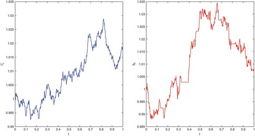
Figure 1 shows typically the differences and relationships between the sample paths of the spot exchange rate in the $FBS$ model and the subdiffusive $FBS$ model.

Figure 1. Comparison of the spot exchange rate’ sample paths in the $\mathit{F}\mathit{B}\mathit{S}$ model (left) and the subdiffusive $\mathit{F}\mathit{B}\mathit{S}$ model (right) for ${\mathit{r}}_{\mathit{d}}\mathbf{=}\mathbf{0.03},{\mathit{r}}_{\mathit{f}}=\mathbf{0.02}\mathbf{,}$ $\mathit{\alpha }\mathbf{=}\mathbf{0.9}\mathbf{,}\mathbf{H}\mathbf{=}\mathbf{0.8},\mathit{\sigma }\mathbf{=}\mathbf{0.1},{\mathit{S}}_{\mathbf{0}}\mathbf{=}\mathbf{1}$.

The rest of the paper proceeds as follows: In Section 2, we provide an analytic pricing formula for the European currency option in the subdiffusive $FBS$ environment and some Greeks of our pricing model are also obtained. Section 3 is devoted to analyze the impact of scaling and long-range dependence on currency option pricing. Moreover, the comparison of our subdiffusive $FBS$ model and traditional models is undertaken in this section. Finally, Section 4 draws the concluding remarks. The proof of Theorems are provided in Appendix.

2. Pricing model for the European call currency option

In this section, we derive a pricing formula for the European call currency option of the subdiffusive $FBS$ model under the following assumptions:

1. We consider two possible investments: (1) a stock whose price satisfies the equation:

(2.1) $S_t=S_{0}exp\left\{(r_d-r_f)T_{\alpha }(t)+\sigma W_{\alpha ,H}(t)\right\},S_0>0,$(2.1)

where $\alpha \in \left(\frac{1}{2},1\right)$, $H\in [\frac{1}{2},1)$, $\alpha +\alpha H>1$, and $r_d,$ and $r_f$ are the domestic and the foreign interest rates, respectively. (2) A money market account:

(2.2) $d{F}_t=r_d{F}_{t}dt,$(2.2)

where $r_d$ shows the domestic interest rate.

• (ii) The stock pays no dividends or other distributions, and all securities are perfectly divisible. There are no penalties to short selling. It is possible to borrow any fraction of the price of a security to buy it or to hold it, at the short-term interest rate. These are the same valuation policy as in the $BS$ model.

• (iii) There are transaction costs that are proportional to the value of the transaction in the underlying stock. Let k denote the round trip transaction cost per unit dollar of transaction. Suppose $U$ shares of the underlying stock are bought $(U>0)$ or sold $(U<0)$ at the price $S_t$, then the transaction cost is given by $\frac{k}{2}\left|U\right|S_t$ in either buying or selling. Moreover, trading takes place only at discrete intervals.

• (iv) The option value is replicated by a replicating portfolio $\mathrm{\Pi }$ with $U(t)$ units of stock and riskless bonds with value $F(t)$. The value of the option must equal the value of the replicating portfolio to reduce (but not to avoid) arbitrage opportunities and be consistent with economic equilibrium.

• (v) The expected return for a hedged portfolio is equal to that from an option. The portfolio is revised every $\mathrm{\Delta }t$ and hedging takes place at equidistant time points with rebalancing intervals of (equal) length $\mathrm{\Delta }t$, where $\mathrm{\Delta }t$ is a finite and fixed, small time-step.

Remark 2.1. From Guo and Yuan (2014), Magdziarz (2009c), we have $E(T_{\alpha }^m(t))=\frac{t^{m\alpha }m!}{\mathrm{\Gamma }(m\alpha +1)}$. Then, by using $\alpha$-self-similar and non-decreasing sample paths of $T_{\alpha }(t)$, we can obtain that $\alpha$-self-similar and non-decreasing sample paths of $T_{\alpha }(t)$,

(2.3) $\begin{array}{c}E\left(\mathrm{\Delta }{T}_{\alpha }(t)\right)=E\left(T_{\alpha }(t+\mathrm{\Delta }t)-T_{\alpha }(t)\right)\\ =\frac{1}{\mathrm{\Gamma }(1+\alpha )}\left[{(t+\mathrm{\Delta }t)}^{\alpha }-t^{\alpha }\right]=\frac{t^{\alpha -1}}{\mathrm{\Gamma }(\alpha )}\mathrm{\Delta }t.\end{array}$(2.3)

and

(2.4) $E\left((\mathrm{\Delta }{B}_H{(T_{\alpha }(t))}^2\right)={\left[\frac{t^{\alpha -1}}{\mathrm{\Gamma }(\alpha )}\right]}^{2H}\mathrm{\Delta }{t}^{2H}.$(2.4)

Let $C=C(t,S_t)$ be the price of a European currency option at time $t$ with a strike price $K$ that matures at time $T$. Then, the pricing formula for currency call option is given by the following theorem.

Theorem 2.1. $C=C(t,S_t)$ is the value of the European currency call option on the stock $S_t$ satisfied (1.5) and the trading takes place discretely with rebalancing intervals of length $\mathrm{\Delta }t$. Then, $C$ satisfies the partial differential equation

(2.5) $\frac{\mathrm{\partial }C}{\mathrm{\partial }t}+(r_d-r_f)S_t\frac{\mathrm{\partial }C}{\mathrm{\partial }{S}_t}+\frac{1}{2}{\hat{\sigma }}^2{S}_t^2\frac{{\mathrm{\partial }}^{2}C}{\mathrm{\partial }{S}_t^2}-r_{d}C=0,$(2.5)

with boundary condition $C(T,S_T)=max\left\{S_T-K,0\right\}$. The value of the currency call option is

(2.6) $C(t,S_t)=S_t{e}^{-r_f(T-t)}\mathrm{\Phi }(d_1)-K{e}^{-r_d(T-t)}\mathrm{\Phi }(d_2),$(2.6)

and the value of the put currency option is

(2.7) $P(t,S_t)=K{e}^{-r_d(T-t)}\mathrm{\Phi }(-d_2)-S_t{e}^{-r_f(T-t)}\mathrm{\Phi }(-d_1),$(2.7)

where

$d_1=\frac{ln\left(\frac{S_t}{K}\right)+\left(r_d-r_f\right)(T-t)+\frac{{\hat{\sigma }}^2}{2}(T-t)}{\hat{\sigma }\sqrt{T-t}},$

(2.8) $d_2=d_1-\hat{\sigma }(t)\sqrt{T-t},$(2.8)

(2.9) ${\hat{\sigma }}^2={\sigma }^2\left[{\left(\frac{t^{\alpha -1}}{\mathrm{\Gamma }(\alpha )}\right)}^{2H}\mathrm{\Delta }{t}^{2H-1}+\sqrt{\frac{2}{\pi }}\frac{k}{\sigma }{\left(\frac{t^{\alpha -1}}{\mathrm{\Gamma }(\alpha )}\right)}^H\mathrm{\Delta }{t}^{H-1}\right],$(2.9)

where $\mathrm{\Phi }(.)$ is the cumulative normal distribution function.

In what follows, the properties of the subdiffusive $FBS$ model are discussed, such as Greeks, which summarize how option prices change with respect to underlying variables and are critically important to asset pricing and risk management. The model can be used to rebalance a portfolio to achieve the desired exposure to certain risk. More importantly, by knowing the Greeks, particular exposure can be hedged from adverse changes in the market by using appropriate amounts of other related financial instruments. In contrast to option prices that can be observed in the market, Greeks cannot be observed and must be calculated given a model assumption. The Greeks are typically computed using a partial differentiation of the price formula.

Theorem 2.2. The Greeks can be written as follows:

(2.10) $\mathrm{\Delta }=\frac{\mathrm{\partial }C}{\mathrm{\partial }{S}_t}=e^{-r_f(T-t)}\mathrm{\Phi }(d_1),$(2.10)

(2.11) $\mathrm{\nabla }=\frac{\mathrm{\partial }C}{\mathrm{\partial }K}=-e^{-r_d(T-t)}\mathrm{\Phi }(d_2),$(2.11)

(2.12) ${\rho }_{r_d}=\frac{\mathrm{\partial }C}{\mathrm{\partial }{r}_d}=K(T-t)e^{-r_d(T-t)}\mathrm{\Phi }(d_2),$(2.12)

(2.13) ${\rho }_{r_f}=\frac{\mathrm{\partial }C}{\mathrm{\partial }{r}_f}=-S_t(T-t)e^{-r_f(T-t)}\mathrm{\Phi }(d_1),$(2.13)

(2.14) $\begin{array}{rl}& \mathrm{\Theta }=\frac{\mathrm{\partial }C}{\mathrm{\partial }t}=S_t{r}_f{e}^{-r_f(T-t)}\mathrm{\Phi }(d_1)-K{r}_d{e}^{-r_d(T-t)}\mathrm{\Phi }(d_2)\\ & +S_t{e}^{-r_f(T-t)}{\sigma }^2(\alpha -1)\frac{t^{\alpha -2}}{\mathrm{\Gamma }(\alpha )}\frac{H{\left(\frac{t^{\alpha -1}}{\mathrm{\Gamma }(\alpha )}\right)}^{2H-1}\mathrm{\Delta }{t}^{2H-1}}{\hat{\sigma }\sqrt{T-t}}(T-t){\mathrm{\Phi }}^{\prime }(d_1)\\ & +S_t{e}^{-r_f(T-t)}\sqrt{\frac{2}{\pi }}k\sigma (\beta -1)\frac{t^{\alpha -2}}{\mathrm{\Gamma }(\alpha )}\frac{H{\left(\frac{t^{\alpha -1}}{\mathrm{\Gamma }(\alpha )}\right)}^{H-1}\mathrm{\Delta }{t}^{H-1}}{2\hat{\sigma }\sqrt{T-t}}(T-t){\mathrm{\Phi }}^{\prime }(d_1)\\ & -S_t{e}^{-r_f(T-t)}\frac{\hat{\sigma }}{2\sqrt{T-t}}{\mathrm{\Phi }}^{\prime }(d_1),\end{array}$(2.14)

(2.15) $\mathrm{\Gamma }=\frac{{\mathrm{\partial }}^{2}C}{\mathrm{\partial }{S}_t^2}=e^{-r_f(T-t)}\frac{{\mathrm{\Phi }}^{\prime }(d_1)}{S_t\hat{\sigma }\sqrt{T-t}},$(2.15)

(2.16) ${\vartheta }_{\hat{\sigma }}=\frac{\mathrm{\partial }C}{\mathrm{\partial }\hat{\sigma }}=S_t{e}^{-r_f(T-t)}\sqrt{T-t}{\mathrm{\Phi }}^{\prime }(d_1).$(2.16)

Remark 2.2. The modified volatility without transaction costs $(k=0)$ is given by

(2.17) ${\hat{\sigma }}^2={\sigma }^2\left[{\left(\frac{t^{\alpha -1}}{\mathrm{\Gamma }(\alpha )}\right)}^{2H}\mathrm{\Delta }{t}^{2H-1}\right],$(2.17)

specially if $\alpha \uparrow 1$,

(2.18) ${\hat{\sigma }}^2={\sigma }^2\mathrm{\Delta }{t}^{2H-1},$(2.18)

which is consistent with the result in Necula (2002).

Furthermore, from Equation (2.18), if $H\downarrow \frac{1}{2}$, then ${\hat{\sigma }}^2={\sigma }^2$, which is according to the results with the $G-K$ model (Garman & Kohlhagen, 1983).

Letting $\alpha \uparrow 1$, from Equation (2.9), we obtain

Remark 2.3. The modified volatility under transaction costs is given by

(2.19) ${\hat{\sigma }}^2={\sigma }^2\left[\mathrm{\Delta }{t}^{2H-1}+\sqrt{\frac{2}{\pi }}\frac{k}{\sigma }\mathrm{\Delta }{t}^{H-1}\right],$(2.19)

that is in line with the findings in Wang (2010).

3. Empirical studies

The objective of this section is to obtain the minimal price of an option with transaction costs and to show the impact of time scaling $\mathrm{\Delta }t$, transaction costs $k$, and subordinator parameter $\alpha$ on the subdiffusive $FBS$ model. Moreover, in the last part, we compute the currency option prices using our model and make comparisons with the results of the $G-K$ and $FBS$ models.

As $\frac{k}{\sigma }<\sqrt{\frac{\pi }{2}}$ often holds (for example: $\sigma =0.1,k=0.01$), from Equation (2.9), we have

(3.1) $\begin{array}{c}\frac{{\hat{\sigma }}^2}{{\sigma }^2}={\left(\frac{t^{\alpha -1}}{\mathrm{\Gamma }(\alpha )}\right)}^{2H}\mathrm{\Delta }{t}^{2H-1}+\sqrt{\frac{2}{\pi }}\frac{k}{\sigma }{\left(\frac{t^{\alpha -1}}{\mathrm{\Gamma }(\alpha )}\right)}^H\mathrm{\Delta }{t}^{H-1}\\ \ge 2{\left(\frac{t^{\alpha -1}}{\mathrm{\Gamma }(\alpha )}\right)}^{\frac{3}{2}H}\mathrm{\Delta }{t}^{\frac{3}{2}H-1}{\left(\frac{2}{\pi }\right)}^{\frac{1}{4}}{\left(\frac{k}{\sigma }\right)}^{\frac{1}{2}},\end{array}$(3.1)

where $H>\frac{1}{2}$. Then, the minimal volatility ${\hat{\sigma }}_{min}$ is $\sqrt{2}\sigma {\left(\frac{t^{\alpha -1}}{\mathrm{\Gamma }(\alpha )}\right)}^{\frac{1}{2}}{\left(\frac{2}{\pi }\right)}^{\frac{1}{2}-\frac{1}{4H}}{\left(\frac{k}{\sigma }\right)}^{1-\frac{1}{2H}}$ as $\mathrm{\Delta }t={\left(\frac{t^{\alpha -1}}{\mathrm{\Gamma }(\alpha )}\right)}^{-1}{\left(\frac{2}{\pi }\right)}^{\frac{1}{2H}}{\left(\frac{k}{\sigma }\right)}^{\frac{1}{H}}$. Thus, the minimal price of an option under transaction costs is represented as $C_{min}(t,S_t)$ with ${\hat{\sigma }}_{min}$ in Equation (2.8).

Moreover, the option rehedging time interval for traders to take is $\mathrm{\Delta }t={\left(\frac{t^{\alpha -1}}{\mathrm{\Gamma }(\alpha )}\right)}^{-1}{\left(\frac{2}{\pi }\right)}^{\frac{1}{2H}}{\left(\frac{k}{\sigma }\right)}^{\frac{1}{H}}$. The minimal price $C_{min}(t,S_t)$ can be used as the actual price of an option.

In particular, as $\mathrm{\Delta }t<1,\alpha \in \left(\frac{1}{2},1\right)$ and $\frac{\mathrm{\partial }C}{\mathrm{\partial }\hat{\sigma }}=S_t{e}^{-r_f(T-t)}\frac{\sqrt{T-t}}{\sqrt{2\pi }}{e}^{-\frac{d^2}{2}}>0,$

(3.2) $\begin{array}{rl}& \frac{\mathrm{\partial }\hat{\sigma }}{\mathrm{\partial }H}=\sigma \left[2{\left(\frac{t^{\alpha -1}}{\mathrm{\Gamma }(\alpha )}\right)}^{2H}\mathrm{\Delta }{t}^{2H-1}+\sqrt{\frac{2}{\pi }}\frac{k}{\sigma }{\left(\frac{t^{\alpha -1}}{\mathrm{\Gamma }(\alpha )}\right)}^H\mathrm{\Delta }{t}^{H-1}\right]\left[ln\left(\frac{t^{\alpha -1}}{\mathrm{\Gamma }(\alpha )}\right)+ln\mathrm{\Delta }t\right]\\ & \times 2{\left[{\left(\frac{t^{\alpha -1}}{\mathrm{\Gamma }(\alpha )}\right)}^{2H}\mathrm{\Delta }{t}^{2H-1}+\sqrt{\frac{2}{\pi }}\frac{k}{\sigma }{\left(\frac{t^{\alpha -1}}{\mathrm{\Gamma }(\alpha )}\right)}^H\mathrm{\Delta }{t}^{H-1}\right]}^{-\frac{1}{2}}\\ & =\left[2{\left(\frac{t^{\alpha -1}}{\mathrm{\Gamma }(\alpha )}\right)}^{2H}\mathrm{\Delta }{t}^{2H-1}+\sqrt{\frac{2}{\pi }}\frac{k}{\sigma }{\left(\frac{t^{\alpha -1}}{\mathrm{\Gamma }(\alpha )}\right)}^H\mathrm{\Delta }{t}^{H-1}\right]\\ & \times \frac{{\sigma }^2\left[ln\left(\frac{t^{\alpha -1}}{\mathrm{\Gamma }(\alpha )}\right)+ln\mathrm{\Delta }t\right]}{2\hat{\sigma }}<0,\end{array}$(3.2)

and $\frac{\mathrm{\partial }C}{\mathrm{\partial }H}=\frac{\mathrm{\partial }C}{\mathrm{\partial }\hat{\sigma }}\frac{\mathrm{\partial }\hat{\sigma }}{\mathrm{\partial }H}$, then we have

(3.3) $\frac{\mathrm{\partial }C}{\mathrm{\partial }H}<0asH\in [\frac{1}{2},1),$(3.3)

which displays that an increasing Hurst exponent comes along with a decrease of the option value (see Figure 2).

Figure 2. Call currency option values.

On the other hand, if $H\downarrow \frac{1}{2}$, then

(3.4) ${\hat{\sigma }}_{min}=\sqrt{2}\sigma {\left(\frac{t^{\alpha -1}}{\mathrm{\Gamma }(\alpha )}\right)}^{\frac{1}{2}}{\left(\frac{2}{\pi }\right)}^{\frac{1}{2}-\frac{1}{4H}}{\left(\frac{k}{\sigma }\right)}^{1-\frac{1}{2H}}\to \sigma \sqrt{2\left(\frac{t^{\alpha -1}}{\mathrm{\Gamma }(\alpha )}\right)}$(3.4)

and if $\alpha \uparrow 1$, then ${\hat{\sigma }}_{min}\to \sqrt{2}\sigma$ as $H\downarrow \frac{1}{2}.$

In addition, if $H\downarrow \frac{1}{2}$

(3.5) $\mathrm{\Delta }t={\left(\frac{t^{\alpha -1}}{\mathrm{\Gamma }(\alpha )}\right)}^{-1}{\left(\frac{2}{\pi }\right)}^{\frac{1}{2H}}{\left(\frac{k}{\sigma }\right)}^{\frac{1}{H}}\to {\left(\frac{t^{\alpha -1}}{\mathrm{\Gamma }(\alpha )}\right)}^{-1}\left(\frac{2}{\pi }\right){\left(\frac{k}{\sigma }\right)}^2,$(3.5)

and if $\alpha \uparrow 1$, then $\mathrm{\Delta }t\to \left(\frac{2}{\pi }\right){\left(\frac{k}{\sigma }\right)}^2$ as $H\downarrow \frac{1}{2}.$

Lux and Marchesi (1999) have shown that Hurst exponent $H=0.51\pm 0.004$ in some cases, so Equations (3.4) and (3.5) have a practical application in option pricing. For example: if $H\downarrow \frac{1}{2},\alpha \uparrow 1,k=2\mathrm{\%}$ and $\sigma =20\mathrm{\%}$, then ${\hat{\sigma }}_{min}\to \frac{\sqrt{2}}{20}$, and $\mathrm{\Delta }t\to \frac{0.02}{\pi }$; and if $H\uparrow \frac{1}{2},\alpha \uparrow 1,k=0.2\mathrm{\%}$ and $\sigma =20\mathrm{\%}$, then ${\hat{\sigma }}_{min}\to \frac{\sqrt{2}}{20}$, and $\mathrm{\Delta }t\to \frac{2}{\pi }\times {10}^{-4}.$

In the following, we investigate the impact of scaling and long-range dependence on option pricing. It is well known that Mantegna and Stanley (1995) introduced the method of scaling invariance from the complex science into the economic systems for the first time. Since then, a lot of research for scaling laws in finance has begun. If $H=\frac{1}{2}$ and $k=0$, from Equation (2.9), we know that ${\hat{\sigma }}^2={\sigma }^2\left(\frac{t^{\alpha -1}}{\mathrm{\Gamma }(\alpha )}\right)$ shows that fractal scaling $\mathrm{\Delta }t$ has not any impact on option pricing if a mean self-financing delta-hedging strategy is applied in a discrete time setting, while subordinator parameter $\beta$ has remarkable impact on option pricing in this case. In particular, from Equations (3.4) and (3.5), we know that ${\hat{\sigma }}_{min}\to \sigma \sqrt{2\left(\frac{t^{\alpha -1}}{\mathrm{\Gamma }(\alpha )}\right)}$ as $H\approx \frac{1}{2}$ and $\mathrm{\Delta }t\to {\left(\frac{t^{\alpha -1}}{\mathrm{\Gamma }(\alpha )}\right)}^{-1}\left(\frac{2}{\pi }\right){\left(\frac{k}{\sigma }\right)}^2,$ as $H\approx \frac{1}{2}$. Therefore, $C_{min}(t,S_t)$ is approximately scaling free with respect to the parameter $k$, if $H\approx \frac{1}{2}$, but is scaling dependent with respect to subordinator parameter $\alpha$. However, $\mathrm{\Delta }t\to {\left(\frac{t^{\alpha -1}}{\mathrm{\Gamma }(\alpha )}\right)}^{-1}\left(\frac{2}{\pi }\right){\left(\frac{k}{\sigma }\right)}^2,$ is scaling dependent with respect to parameters $k$ and $\alpha$, if $H\approx \frac{1}{2}$. On the other hand, if $H>\frac{1}{2}$ and $k=0$, from Equation (2.17), we know that ${\hat{\sigma }}^2={\sigma }^2\left[{\left(\frac{t^{\alpha -1}}{\mathrm{\Gamma }(\alpha )}\right)}^{2H}\mathrm{\Delta }{t}^{2H-1}\right]$, which displays that the fractal scaling $\mathrm{\Delta }t$ and sabordinator parameter $\alpha$ have a significant impact on option pricing. Furthermore, for $k\ne 0$, from Equation (2.8), we know that option pricing is scaling dependent in general.

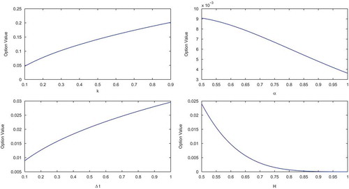
Now, we present the values of currency call option using subdiffusive $FBS$ model for different parameters. For the sake of simplicity, we will just consider the out-of-the-money case. Indeed, using the same method, one can also discuss the remaining cases: in-the-money and at-the-money. First, the prices of our subdiffusive $FBS$ model are investigated for some $\mathrm{\Delta }t$ and prices for different exponent parameters. The prices of the call currency option versus its parameters $H,\mathrm{\Delta }t,\alpha$ and $k$ are revealed in Figure 2. The selected parameters are $S_t=1.4,K=1.5,\sigma =0.1,r_d=0.03,r_f=0.02,T=1,t=0.1,\mathrm{\Delta }t=0.01,k=0.01,H=0.8,\alpha =\mathrm{0.9.}$ Figure 2 indicates that the option price is an increasing function of $k$ and $\mathrm{\Delta }t$, while it is a decreasing function of $H$ and $\alpha$.

For a detailed analysis of our model, the prices calculated by the $G-K$, $FBS$ and subdiffusive $FBS$ models are compared for both out-of-the-money and in-the-money cases. The following parameters are chosen: $S_t=1.2,\sigma =0.5,r_d=0.05,r_f=0.01,t=0.1,\mathrm{\Delta }t=0.01,k=0.001$, and $H=0.8$, along with time maturity $T\in [0.1,2]$, strike price $K\in [0.8,1.19]$ for the in-the-money case and $K\in [1.21,1.4]$ for the out-of-the-money case. Figures 3 and 4 show the theoretical values difference by the $G-K$, $FBS$, and our subdiffusive $FBS$ models for the in-the-money and out-of-the-money, respectively. As indicated in these figures, the values computed by our subdiffusive $FBS$ model are better fitted to the $G-K$ values than the $FBS$ model for both in-the-money and out-of-the money cases. Hence, when compared to these figures, our subdiffusive $FBS$ model seems reasonable.

Figure 3. Relative difference between the $\mathit{G}\mathbf{-}\mathit{K}$, $\mathit{F}\mathit{B}\mathit{S}$, and subdiffusive $\mathit{F}\mathit{B}\mathit{S}$ models for the in-the-money case.

Figure 4. Relative difference between the $\mathit{G}\mathbf{-}\mathit{K}$, $\mathit{F}\mathit{B}\mathit{S}$, and subdiffusive $\mathit{F}\mathit{B}\mathit{S}$ models for the out-of-the-money case.

4. Conclusion

Without using the arbitrage argument, in this paper, we derive a European currency option pricing model with transaction costs to capture the behavior of the spot exchange rate price, where the spot exchange rate follows a subdiffusive $FBS$ with transaction costs. In discrete time case, we show that the time scaling $\mathrm{\Delta }t$ and the Hurst exponent $H$ play an important role in option pricing with or without transaction costs and option pricing is scaling dependent. In particular, the minimal price of an option under transaction costs is obtained.

Acknowledgments

I would like to thank the referees and the editor for their careful reading and their valuable comments.

Additional information

Funding

The author received no direct funding for this research. This paper is supported by the university of Vaasa, Finland.

Notes on contributors

Foad Shokrollahi

Foad Shokrollahi is a researcher at Department of Mathematics and Statistics, University of Vaasa, Finland. His research interests are Stochastic Processes, Stochastic Analysis, Fractional Brownian motion, and Mathematical Finance.

Appendix

Proof of Theorem 2.1. The movement of $S_t$ on time interval $[t,t+\mathrm{\Delta }t)$ of length $\mathrm{\Delta }t$ is

(4.1) $\begin{array}{rl}& \mathrm{\Delta }{S}_t=S_{t+\mathrm{\Delta }t}-S_t=S_t(e^{(r_d-r_f)\mathrm{\Delta }{T}_{\alpha }(t)+\sigma \mathrm{\Delta }{W}_{\alpha ,H}(t)}-1)\\ & =S_t((r_d-r_f)\mathrm{\Delta }{T}_{\alpha }(t)+\sigma \mathrm{\Delta }{W}_{\alpha ,H}(t)\\ & +\frac{1}{2}((r_d-r_f)\mathrm{\Delta }{T}_{\alpha }(t)+\sigma \mathrm{\Delta }{W}_{\alpha ,H}(t){)}^2)\\ & +\frac{1}{6}{S}_t{e}^{[\theta ((r_d-r_f)\mathrm{\Delta }{T}_{\alpha }(t)+\sigma \mathrm{\Delta }{W}_{\alpha ,H}(t))]}\\ & \times ((r_d-r_f)\mathrm{\Delta }{T}_{\alpha }(t)+\sigma \mathrm{\Delta }{W}_{\alpha ,H}(t){)}^3,\end{array}$(4.1)

here $\theta =\theta (t,\mathrm{\Delta }t)\in (0,1)$ is a random variable corresponding to process $S_t$.

Based on Lemmas 2.1 and 2.2 of Gu et al. (2012), we can get

(4.2) $\begin{array}{rl}& ((r_d-r_f)\mathrm{\Delta }{T}_{\alpha }(t)+\sigma \mathrm{\Delta }{W}_{\alpha ,H}(t){)}^2=(o(\mathrm{\Delta }{t}^{\alpha -\epsilon })+o(\mathrm{\Delta }{t}^{\alpha H-\epsilon }){)}^2\\ & =o(\mathrm{\Delta }{t}^{\alpha +\alpha H-2\epsilon })+o(\mathrm{\Delta }{t}^{2\alpha H-2\epsilon }),\end{array}$(4.2)

(4.3) $\begin{array}{rl}& e^{[\theta ((r_d-r_f)\mathrm{\Delta }{T}_{\alpha }(t)+\sigma \mathrm{\Delta }{W}_{\alpha ,H}(t))]}((r_d-r_f)\mathrm{\Delta }{T}_{\alpha }(t)+\sigma \mathrm{\Delta }{W}_{\alpha ,H}(t){)}^3\\ & =o(\mathrm{\Delta }{t}^{3\alpha -3\epsilon })+o(\mathrm{\Delta }{t}^{2\alpha +\alpha H-3\epsilon })+o(\mathrm{\Delta }{t}^{2\alpha H+\alpha -3\epsilon })+o(\mathrm{\Delta }{t}^{3\alpha -3\epsilon })\\ & =o(\mathrm{\Delta }{t}^{3\alpha H-3\epsilon }),\end{array}$(4.3)

(4.4) $o(\mathrm{\Delta }{t}^{\alpha +\alpha H-2\epsilon })+o(\mathrm{\Delta }{t}^{3\alpha H-3\epsilon })=o(\mathrm{\Delta }{t}^{\alpha +\alpha H-2\epsilon }).$(4.4)

From the above equations, Equation (4.1) can be rewritten as follows

(4.5) $\begin{array}{rl}& \mathrm{\Delta }{S}_t=(r_d-r_f)S_t\mathrm{\Delta }{T}_{\alpha }(t)+\sigma S_t\mathrm{\Delta }{W}_{\alpha ,H}(t)\\ & +\frac{1}{2}{\sigma }^2{S}_t(\mathrm{\Delta }{W}_{\alpha ,H}(t){)}^2+o(\mathrm{\Delta }{t}^{\alpha +\alpha H-2\epsilon }).\end{array}$(4.5)

By the assumption $\alpha H+\alpha >1$, we obtain

(4.6) $\mathrm{\Delta }{S}_t=(r_d-r_f)S_t\mathrm{\Delta }{T}_{\alpha }(t)+\sigma S_t\mathrm{\Delta }{W}_{\alpha ,H}(t)$(4.6)

Applying the Taylor expansion to $C(t,S_t)$, we have

(4.7) $\begin{array}{rl}& \mathrm{\Delta }C(t,S_t)=\frac{\mathrm{\partial }C}{\mathrm{\partial }t}\mathrm{\Delta }t+\frac{\mathrm{\partial }C}{\mathrm{\partial }{S}_t}\mathrm{\Delta }{S}_t+\frac{1}{2}\frac{{\mathrm{\partial }}^{2}C}{\mathrm{\partial }{S}_t^2}\mathrm{\Delta }{S}_t^2\\ & +\frac{1}{2}\frac{{\mathrm{\partial }}^{2}C}{\mathrm{\partial }{t}^2}\mathrm{\Delta }{t}^2+\frac{{\mathrm{\partial }}^{2}C}{\mathrm{\partial }{S}_t\mathrm{\partial }t}\mathrm{\Delta }t\mathrm{\Delta }{S}_t+o(\mathrm{\Delta }{t}^{3\alpha H-\epsilon })\\ & =\frac{\mathrm{\partial }C}{\mathrm{\partial }t}\mathrm{\Delta }t+\frac{\mathrm{\partial }C}{\mathrm{\partial }{S}_t}\mathrm{\Delta }{S}_t+\frac{1}{2}\frac{{\mathrm{\partial }}^{2}C}{\mathrm{\partial }{S}_t^2}\mathrm{\Delta }{S}_t^2+o(\mathrm{\Delta }t)\\ & =\frac{\mathrm{\partial }C}{\mathrm{\partial }t}\mathrm{\Delta }t+(r_d-r_f)S_t\frac{\mathrm{\partial }C}{\mathrm{\partial }{S}_t}\mathrm{\Delta }{T}_{\alpha }(t)+\sigma S_t\frac{\mathrm{\partial }C}{\mathrm{\partial }{S}_t}\mathrm{\Delta }{W}_{\alpha ,H}(t)\\ & +\frac{1}{2}{\sigma }^2{S}_t\frac{\mathrm{\partial }C}{\mathrm{\partial }{S}_t}(\mathrm{\Delta }{W}_{\alpha ,H}(t){)}^2\\ & +\frac{1}{2}{\sigma }^2{S}_t^2\frac{{\mathrm{\partial }}^{2}C}{\mathrm{\partial }{S}_t^2}(\mathrm{\Delta }{W}_{\alpha ,H}(t){)}^2+o(\mathrm{\Delta }t).\end{array}$(4.7)

From Equations (4.1)–(4.5), we obtain that $\frac{{\mathrm{\partial }}^{2}C}{\mathrm{\partial }{S}_t^2}$, $\frac{{\mathrm{\partial }}^{3}C}{\mathrm{\partial }{S}_t^3}$, $\frac{{\mathrm{\partial }}^{2}C}{\mathrm{\partial }C\mathrm{\partial }t}$ is $o(\mathrm{\Delta }{t}^{\frac{1}{2}{(1-H\alpha )}^{-\epsilon }})$ and

(4.8) $\mathrm{\Delta }\left(\frac{\mathrm{\partial }C}{\mathrm{\partial }{S}_t}\right)=\frac{{\mathrm{\partial }}^{2}C}{\mathrm{\partial }{S}_t\mathrm{\partial }t}\mathrm{\Delta }t+\frac{{\mathrm{\partial }}^{2}C}{\mathrm{\partial }{S}_t^2}\mathrm{\Delta }{S}_t+\frac{1}{2}\frac{{\mathrm{\partial }}^{3}C}{\mathrm{\partial }{S}_t^3}\mathrm{\Delta }{S}_t^2+o(\mathrm{\Delta }t),$(4.8)

and

(4.9) $\left|\mathrm{\Delta }\left(\frac{\mathrm{\partial }C}{\mathrm{\partial }{S}_t}\right)\right|.S_{t+\mathrm{\Delta }t}=\sigma S_t^2\left|\frac{{\mathrm{\partial }}^{2}C}{\mathrm{\partial }{S}_t^2}\right|\left|\mathrm{\Delta }{W}_{\alpha ,H}(t)\right|+o(\mathrm{\Delta }t).$(4.9)

Moreover, from assumptions (iii) and (iv), it is found that the change in the value of portfolio ${\mathrm{\Pi }}_t$ is

(4.10) $\begin{array}{c}\mathrm{\Delta }{\mathrm{\Pi }}_t=U_t(\mathrm{\Delta }{S}_t+r_f{S}_t\mathrm{\Delta }t)+\mathrm{\Delta }{F}_t-\frac{k}{2}\left|\mathrm{\Delta }{U}_t\right|S_{t+\mathrm{\Delta }t}\\ =U_t(\mathrm{\Delta }{S}_t+r_f{S}_t\mathrm{\Delta }t)+r_d{F}_t\mathrm{\Delta }t\\ -\frac{k}{2}\left|\mathrm{\Delta }{U}_t\right|S_{t+\mathrm{\Delta }t}+o(\mathrm{\Delta }t),\end{array}$(4.10)

where the number of bonds $U_t$ is constant during time-step $\mathrm{\Delta }t$. From assumption (v), $C(t,S_t)$ is replicated by portfolio $\mathrm{\Pi }(t)$. Thus, at time points $\mathrm{\Delta }t$, $2\mathrm{\Delta }t$, $3\mathrm{\Delta }t,...,$ we have $C(t,S_t)=U_t{S}_t+F_t$ and $U_t=\frac{\mathrm{\partial }C}{\mathrm{\partial }{S}_t}$. Therefore, according to Equations (4.5)–(4.10), we have

(4.11) $\begin{array}{rl}& \mathrm{\Delta }\mathrm{\Pi }=\frac{\mathrm{\partial }C}{\mathrm{\partial }{S}_t}\left[(r_d-r_f)S_t\mathrm{\Delta }{T}_{\alpha }(t)+\sigma S_t\mathrm{\Delta }{W}_{\alpha ,H}(t)+\frac{1}{2}{\sigma }^2{S}_t{(\mathrm{\Delta }{W}_{\alpha ,H}(t))}^2+r_f{S}_t\mathrm{\Delta }t\right]\\ & +r_d{F}_t\mathrm{\Delta }t-\frac{k}{2}\left|\mathrm{\Delta }\left(\frac{\mathrm{\partial }C}{\mathrm{\partial }{S}_t}\right)\right|.S_{t+\mathrm{\Delta }t}+o(\mathrm{\Delta }t)\\ & =\frac{\mathrm{\partial }C}{\mathrm{\partial }{S}_t}\left[(r_d-r_f)S_t\mathrm{\Delta }{T}_{\alpha }(t)+\sigma S_t\mathrm{\Delta }{W}_{\alpha ,H}(t)+\frac{1}{2}{\sigma }^2{S}_t{(\mathrm{\Delta }{W}_{\alpha ,H}(t))}^2+r_f{S}_t\mathrm{\Delta }t\right]\\ & +\left(C\left(t,S_t\right)-S_t\frac{\mathrm{\partial }C}{\mathrm{\partial }{S}_t}\right)r_d\mathrm{\Delta }t-\frac{k}{2}\sigma S_t^2\left|\frac{{\mathrm{\partial }}^{2}C}{\mathrm{\partial }{S}_t^2}\right|\mathrm{\Delta }{W}_{\alpha ,H}(t)+o(\mathrm{\Delta }t).\end{array}$(4.11)

Consequently,

(4.12) $\begin{array}{rl}& \mathrm{\Delta }\mathrm{\Pi }-\mathrm{\Delta }C=\left(r_{d}C-\left(r_d-r_f\right)S_t\frac{\mathrm{\partial }C}{\mathrm{\partial }{S}_t}-\frac{\mathrm{\partial }C}{\mathrm{\partial }t}\right)\mathrm{\Delta }t-\frac{1}{2}{\sigma }^2{S}_t^2\frac{{\mathrm{\partial }}^{2}C}{\mathrm{\partial }{S}_t^2}{\left(\mathrm{\Delta }{W}_{\alpha ,H}(t)\right)}^2\\ & -\frac{k}{2}\sigma S_t^2\left|\frac{{\mathrm{\partial }}^{2}C}{\mathrm{\partial }{S}_t^2}\right|\mathrm{\Delta }{W}_{\alpha ,H}(t)+o(\mathrm{\Delta }t).\end{array}$(4.12)

The time subscript, $t$, has been suppressed. As expected, using Equation (4.12), (iv), Remark 2.1, and (4.13), we infer

(4.13) $\begin{array}{rl}& E(\mathrm{\Delta }\mathrm{\Pi }-\mathrm{\Delta }C)=\left(r_{d}C-\left(r_d-r_f\right)S_t\frac{\mathrm{\partial }C}{\mathrm{\partial }{S}_t}-\frac{\mathrm{\partial }C}{\mathrm{\partial }t}\right)\mathrm{\Delta }t\\ & -\frac{1}{2}{\left[\frac{t^{\alpha -1}}{\mathrm{\Gamma }(\alpha )}\right]}^{2H}\mathrm{\Delta }{t}^{2H}{\sigma }^2{S}_t^2\frac{{\mathrm{\partial }}^{2}C}{\mathrm{\partial }{S}_t^2}-\frac{1}{2}\sqrt{\frac{2}{\pi }}k\sigma S_t^2{\left[\frac{t^{\alpha -1}}{\mathrm{\Gamma }(\alpha )}\right]}^H\mathrm{\Delta }{t}^H\left|\frac{{\mathrm{\partial }}^{2}C}{\mathrm{\partial }{S}_t^2}\right|\\ & =\left(r_{d}C-(r_d-r_f)S_t\frac{\mathrm{\partial }C}{\mathrm{\partial }{S}_t}-\frac{\mathrm{\partial }C}{\mathrm{\partial }t}-\frac{1}{2}{\left[\frac{t^{\alpha -1}}{\mathrm{\Gamma }(\alpha )}\right]}^{2H}\mathrm{\Delta }{t}^{2H-1}{\sigma }^2{S}_t^2\frac{{\mathrm{\partial }}^{2}C}{\mathrm{\partial }{S}_t^2}\right.\\ & \left.-\frac{1}{2}\sqrt{\frac{2}{\pi }}k\sigma S_t^2{\left[\frac{t^{\alpha -1}}{\mathrm{\Gamma }(\alpha )}\right]}^H\mathrm{\Delta }{t}^{H-1}\left|\frac{{\mathrm{\partial }}^{2}C}{\mathrm{\partial }{S}_t^2}\right|\right)\mathrm{\Delta }t=0.\end{array}$(4.13)

Thus, from Equation (4.13), we can derive

(4.14) $\begin{array}{rl}& r_{d}C=(r_d-r_f)S_t\frac{\mathrm{\partial }C}{\mathrm{\partial }{S}_t}+\frac{\mathrm{\partial }C}{\mathrm{\partial }t}+\frac{1}{2}{\left[\frac{t^{\alpha -1}}{\mathrm{\Gamma }(\alpha )}\right]}^{2H}\mathrm{\Delta }{t}^{2H-1}{\sigma }^2{S}_t^2\frac{{\mathrm{\partial }}^{2}C}{\mathrm{\partial }{S}_t^2}\\ & +\frac{1}{2}\sqrt{\frac{2}{\pi }}k\sigma S_t^2{\left[\frac{t^{\alpha -1}}{\mathrm{\Gamma }(\alpha )}\right]}^H\mathrm{\Delta }{t}^{H-1}\left|\frac{{\mathrm{\partial }}^{2}C}{\mathrm{\partial }{S}_t^2}\right|.\end{array}$(4.14)

We define ${\hat{\sigma }}^2(t)$ as follows:

(4.15) ${\hat{\sigma }}^2={\sigma }^2\left({\left[\frac{t^{\alpha -1}}{\mathrm{\Gamma }(\alpha )}\right]}^{2H}\mathrm{\Delta }{t}^{2H-1}+\sqrt{\frac{2}{\pi }}k{\sigma }^{-1}{\left[\frac{t^{\alpha -1}}{\mathrm{\Gamma }(\alpha )}\right]}^H\mathrm{\Delta }{t}^{H-1}\right).$(4.15)

where $\frac{{\mathrm{\partial }}^{2}C}{\mathrm{\partial }{S}_t^2}$ is ever positive for the ordinary European currency call option without transaction costs, if the same conduct of $\frac{{\mathrm{\partial }}^{2}C}{\mathrm{\partial }{S}_t^2}$ is postulated here and $\hat{\sigma }(t)$ remains fixed during the time-step $[t,\mathrm{\Delta }t)$. Then, from Equations (4.14) and (4.15), we obtain

(4.16) $\frac{\mathrm{\partial }C}{\mathrm{\partial }t}+(r_d-r_f)S_t\frac{\mathrm{\partial }C}{\mathrm{\partial }{S}_t}+\frac{1}{2}{\hat{\sigma }}^2{S}_t^2\frac{{\mathrm{\partial }}^{2}C}{\mathrm{\partial }{S}_t^2}-r_{d}C=0.$(4.16)

Followed by

(4.17) $C=C(t,S_t)=S_t{e}^{-r_f(T-t)}\mathrm{\Phi }(d_1)-K{e}^{-r_d(T-t)}\mathrm{\Phi }(d_2),$(4.17)

and

(4.18) $\begin{array}{c}{d}_1=\frac{ln\left(\frac{S_t}{K}\right)+(r_d-r_f)(T-t)+\frac{{\hat{\sigma }}^2}{2}(T-t)}{\hat{\sigma }\sqrt{T-t}},\\ \\ d_2=d_1-\hat{\sigma }\sqrt{T-t}.\end{array}$(4.18)

Proof of Theorem 2.2. First, we derive a general formula. Let $y$ be one of the influence factors. Thus

(4.19) $\begin{array}{c}\frac{\mathrm{\partial }C}{\mathrm{\partial }y}=\frac{\mathrm{\partial }{S}_t{e}^{-\left(r_f\right)(T-t)}}{\mathrm{\partial }y}\mathrm{\Phi }(d_1)+S_t{e}^{-r_f(T-t)}\frac{\mathrm{\partial }\mathrm{\Phi }(d_1)}{\mathrm{\partial }y}\\ -\frac{\mathrm{\partial }K{e}^{-r_d(T-t)}}{\mathrm{\partial }y}\mathrm{\Phi }(d_2)-K{e}^{-r_d(T-t)}\frac{\mathrm{\partial }\mathrm{\Phi }(d_2)}{\mathrm{\partial }y}\end{array}$(4.19)

But

(4.20) $\begin{array}{rl}& \frac{\mathrm{\partial }\mathrm{\Phi }(d_2)}{\mathrm{\partial }y}={\mathrm{\Phi }}^{\prime }(d_2)\frac{\mathrm{\partial }{d}_2}{\mathrm{\partial }y}\\ & =\frac{1}{\sqrt{2\pi }}{e}^{-\frac{d_2^2}{2}}\frac{\mathrm{\partial }{d}_2}{\mathrm{\partial }y}\\ & =\frac{1}{\sqrt{2\pi }}exp\left(-\frac{{(d_1-\hat{\sigma }\sqrt{T-t})}^2}{2}\right)\frac{\mathrm{\partial }{d}_2}{\mathrm{\partial }y}\\ & =\frac{1}{\sqrt{2\pi }}{e}^{-\frac{d_1^2}{2}}exp(d_1\hat{\sigma }\sqrt{T-t)})exp\left(-\frac{{\hat{\sigma }}^2(T-t)}{2}\right)\frac{\mathrm{\partial }{d}_2}{\mathrm{\partial }y}\\ & =\frac{1}{\sqrt{2\pi }}{e}^{-\frac{d_1^2}{2}}exp\left(ln\frac{S_t}{K}+(r_d-r_f)(T-t)\right)\frac{\mathrm{\partial }{d}_2}{\mathrm{\partial }y}\\ & =\frac{1}{\sqrt{2\pi }}{e}^{-\frac{d_1^2}{2}}\frac{S}{K}exp((r_d-r_f)(T-t))\frac{\mathrm{\partial }{d}_2}{\mathrm{\partial }y}.\end{array}$(4.20)

Then

(4.21) $\begin{array}{c}\frac{\mathrm{\partial }C}{\mathrm{\partial }y}=\frac{\mathrm{\partial }{S}_t{e}^{-(r_f)(T-t)}}{\mathrm{\partial }y}\mathrm{\Phi }(d_1)-\frac{\mathrm{\partial }K{e}^{-r_d(T-t)}}{\mathrm{\partial }y}\mathrm{\Phi }(d_2)\\ +S_t{e}^{-r_f(T-t)}{\mathrm{\Phi }}^{\prime }(d_1)\frac{\mathrm{\partial }\hat{\sigma }\sqrt{T-t)}}{\mathrm{\partial }y}.\end{array}$(4.21)

Substituting in (4.21), we get the desired Greeks.

References

- Borovkov, K., Mishura, Y., Novikov, A., & Zhitlukhin, M. (2018). New and refined bounds for expected maxima of fractional Brownian motion. Statistics & Probability Letters, 137, 142–147. doi:10.1016/j.spl.2018.01.025
- Cheridito, P. (2003). Arbitrage in fractional Brownian motion models. Finance and Stochastics, 7(4), 533–553. doi:10.1007/s007800300101
- Dai, Q., & Singleton, K. J. (2000). Specification analysis of affine term structure models. The Journal of Finance, 55(5), 1943–1978. doi:10.1111/0022-1082.00278
- Ekvall, N., Jennergren, L. P., & Näslund, B. (1997). Currency option pricing with mean reversion and uncovered interest parity: A revision of the Garman-Kohlhagen model. European Journal of Operational Research, 100(1), 41–59. doi:10.1016/S0377-2217(95)00366-5
- Garman, M. B., & Kohlhagen, S. W. (1983). Foreign currency option values. Journal of International Money and Finance, 2(3), 231–237. doi:10.1016/S0261-5606(83)80001-1
- Gu, H., Liang, J.-R., & Zhang, Y.-X. (2012). Time-changed geometric fractional Brownian motion and option pricing with transaction costs. Physica A: Statistical Mechanics and Its Applications, 391(15), 3971–3977. doi:10.1016/j.physa.2012.03.020
- Guo, Z. (2017). Option pricing under the merton model of the short rate in subdiffusive Brownian motion regime. Journal of Statistical Computation and Simulation, 87(3), 519–529. doi:10.1080/00949655.2016.1218880
- Guo, Z., & Yuan, H. (2014). Pricing European option under the time-changed mixed Brownian-fractional Brownian model. Physica A: Statistical Mechanics and Its Applications, 406, 73–79. doi:10.1016/j.physa.2014.03.032
- Ho, T. S., Stapleton, R. C., & Subrahmanyam, M. G. (1995). Correlation risk, cross-market derivative products and portfolio performance. European Financial Management, 1(2), 105–124. doi:10.1111/j.1468-036X.1995.tb00011.x
- Janczura, J., Orzeł, S., & Wyłomańska, A. (2011). Subordinated α-stable Ornstein–Uhlenbeck process as a tool for financial data description. Physica A: Statistical Mechanics and Its Applications, 390(23–24), 4379–4387. doi:10.1016/j.physa.2011.07.007
- Janicki, A., & Weron, A. (1993). Simulation and chaotic behavior of alpha-stable stochastic processes (Vol. 178). CRC Press.
- Janicki, A., & Weron, A. (1995). Simulation and chaotic behaviour of a-stable stochastic processes. Journal of the Royal Statistical Society-Series A Statistics in Society, 158(2), 339.
- Karipova, G., & Magdziarz, M. (2017). Pricing of basket options in subdiffusive fractional Black–Scholes model. Chaos, Solitons & Fractals, 102, 245–253. doi:10.1016/j.chaos.2017.05.013
- Kumar, A., Wyłomańska, A., Połoczański, R., & Sundar, S. (2017). Fractional Brownian motion time-changed by gamma and inverse gamma process. Physica A: Statistical Mechanics and Its Applications, 468, 648–667. doi:10.1016/j.physa.2016.10.060
- Lux, T., & Marchesi, M. (1999). Scaling and criticality in a stochastic multi-agent model of a financial market. Nature, 397(6719), 498–500. doi:10.1038/17290
- Magdziarz, M. (2009a). Black-Scholes formula in subdiffusive regime. Journal of Statistical Physics, 136(3), 553–564. doi:10.1007/s10955-009-9791-4
- Magdziarz, M. (2009b). Langevin picture of subdiffusion with infinitely divisible waiting times. Journal of Statistical Physics, 135(4), 763–772. doi:10.1007/s10955-009-9751-z
- Magdziarz, M. (2009c). Stochastic representation of subdiffusion processes with time-dependent drift. Stochastic Processes and Their Applications, 119(10), 3238–3252. doi:10.1016/j.spa.2009.05.006
- Magdziarz, M. (2010). Path properties of subdiffusiona martingale approach. Stochastic Models, 26(2), 256–271. doi:10.1080/15326341003756379
- Magdziarz, M., Weron, A., & Weron, K. (2007). Fractional Fokker-Planck dynamics: Stochastic representation and computer simulation. Physical Review E, 75(1), 016708. doi:10.1103/PhysRevE.75.016708
- Mantegna, R. N., Stanley, H. E. (1995). Scaling behaviour in the dynamics of an economic index. Nature, 376(6535), 46–49. doi:10.1038/376046a0
- Mastinšek, M. (2006). Discrete–time delta hedging and the Black–Scholes model with transaction costs. Mathematical Methods of Operations Research, 64(2), 227–236. doi:10.1007/s00186-006-0086-0
- Metzler, R., & Klafter, J. (2000). The random walk’s guide to anomalous diffusion: A fractional dynamics approach. Physics Reports, 339(1), 1–77. doi:10.1016/S0370-1573(00)00070-3
- Necula, C. (2002).Option pricing in a fractional Brownian motion environment. Available at SSRN 1286833.
- Piryatinska, A., Saichev, A., & Woyczynski, W. (2005). Models of anomalous diffusion: The subdiffusive case. Physica A: Statistical Mechanics and Its Applications, 349(3–4), 375–420. doi:10.1016/j.physa.2004.11.003
- Scalas, E., Gorenflo, R., & Mainardi, F. (2000). Fractional calculus and continuous-time finance. Physica A: Statistical Mechanics and Its Applications, 284(1–4), 376–384. doi:10.1016/S0378-4371(00)00255-7
- Shokrollahi, F., & Kılıçman, A. (2014). Delta-hedging strategy and mixed fractional Brownian motion for pricing currency option. Mathematical Problems in Engineering, 501, 718768.
- Shokrollahi, F., & Kılıçman, A. (2014). Pricing currency option in a mixed fractional Brownian motion with jumps environment. Mathematical Problems in Engineering, 2014, 1–13. doi:10.1155/2014/858210
- Shokrollahi, F., & Sottinen, T. (2017). Hedging in fractional Black–Scholes model with transaction costs. Statistics & Probability Letters, 130, 85–91. doi:10.1016/j.spl.2017.07.014
- Sottinen, T., & Valkeila, E. (2003). On arbitrage and replication in the fractional Black–Scholes pricing model. Statistics & Decisions/International Mathematical Journal for Stochastic Methods and Models, 21(2/2003), 93–108.
- Wang, X.-T. (2010). Scaling and long-range dependence in option pricing I: Pricing European option with transaction costs under the fractional Black–Scholes model. Physica A: Statistical Mechanics and Its Applications, 389(3), 438–444. doi:10.1016/j.physa.2009.09.041
- Wang, X.-T., Zhu, E.-H., Tang, -M.-M., & Yan, H.-G. (2010). Scaling and long-range dependence in option pricing II: Pricing European option with transaction costs under the mixed Brownian–fractional Brownian model. Physica A: Statistical Mechanics and Its Applications, 389(3), 445–451. doi:10.1016/j.physa.2009.09.043
- Xiao, W.-L., Zhang, W.-G., Zhang, X.-L., & Wang, Y.-L. (2010). Pricing currency options in a fractional Brownian motion with jumps. Economic Modelling, 27(5), 935–942. doi:10.1016/j.econmod.2010.05.010
- Yang, Z. (2017). A new factorization of American fractional lookback option in a mixed jump-diffusion fractional Brownian motion environment. Journal of Modeling and Optimization, 9(1), 53–68.
Appendix
Proof of Theorem 2.1. The movement of on time interval
of length
is
here is a random variable corresponding to process
.
Based on Lemmas 2.1 and 2.2 of Gu et al. (Citation2012), we can get